Lepton Masses and Mixing in a Left-Right Symmetric Model with a TeV-scale Gravity

Abstract

We construct a left-right symmetric (LRS) model in five dimensions which accounts naturally for the lepton flavor parameters. The fifth dimension is described by an orbifold, $S_{1}/Z_{2}\times Z^{\prime}_{2}$, with a typical size of order TeV^-1. The fundamental scale is of order 25 TeV which implies that the gauge hierarchy problem is ameliorated. In addition the LRS breaking scale is of order few TeV which implies that interactions beyond those of the standard model are accessible to near future experiments. Leptons of different representations are localized around different orbifold fixed points. This explains, through the Arkani-Hamed-Schmaltz mechanism, the smallness of the tau mass compared to the electroweak breaking scale. An additional U(1) horizontal symmetry, broken by small parameters, yields the hierarchy in the charged lepton masses, strong suppression of the light neutrino masses and accounts for the mixing parameters. The model yields several unique predictions. In particular, the branching ratio for the lepton flavor violating process $\mu^{-}\to e^{+}e^{-}e^{-}$ is comparable with its present experimental sensitivity.

I Introduction

The recent results from the SNO [1] and other [2] experiments provide strong evidences for the incompleteness of the standard model (SM). Among the various new physics (NP) scenarios that predict neutrino masses, the left-right symmetric (LRS) framework [3] is an attractive and popular one.

In many LRS models, e.g. models embedded in GUT [4], the LRS breaking scale, $v_{R}\ \hbox to0.0pt{\raise 3.0pt\hbox{$>$}\hss}{\lower 3.0pt\hbox{$\sim$}}\ 10^{14}{\rm~{}GeV}$, is much higher than the electroweak (EW) breaking scale, $k_{1}\sim 10^{2}{\rm~{}GeV}$, and the low energy effective Lagrangian is similar in many aspects to that of the SM. In such a case present and near future experiments will not be able to directly probe the NP. Furthermore, the introduction of such a high scale, in addition to the Planck scale, $M_{P}\sim 10^{19}{\rm~{}GeV}$, related to gravity in four dimensions, raises the gauge hierarchy and fine tuning problems shared by many models.

A new exciting possibility, however, that the fundamental scale of gravity can in fact be much smaller than $M_{P}$ was raised in [5]. It is very interesting, therefore, to investigate whether a natural LRS model (LRSM), in which both $M_{P}$ and $v_{R}$ are low, say below 100 TeV, and in which the neutrinos are very light, can be constructed.

This work is focused on the lepton flavor parameters, we comment on the inclusion of the quark sector in the conclusion. We present a LRSM which naturally accounts for the flavor parameters of the lepton sector and in which the fundamental scale and the LRS breaking scale are of the order of or below 25 TeV. It is a model of, at least,  one extra compact dimension which copes with the above problems by using both the Froggatt-Nielsen [6] and the Arkani-Hamed-Schmaltz (AS) [7] mechanisms. The main role of the AS mechanism is to localize “left” and “right” lepton fields on different fixed points in the extra dimension, which then explains the smallness of $m_{\tau}$ compared with the electroweak breaking scale. An additional U(1) horizontal symmetry, described in detail in [8], yields a modified see-saw mechanism and accounts for the other flavor parameters.

Before proceeding with the details of our work we note that recent two papers, by Mimura and Nandi [9] and by Mohapatra and Perez-Lorenzana [10], dealt with the construction of a LRSM in five dimensions [5D]. Though important parts of the analysis in [9, 10] are general and also used below the three models use, in fact, different constructions in the extra dimension. Furthermore, to the best of our knowledge, the present model is the only LRSM in 5D that aims to account naturally for all the lepton flavor parameters.

To make our discussion concrete we briefly list the lepton flavor parameters as deduced from various experiments. The charged lepton masses are [11],

$$m_{e}\simeq 5.1\cdot 10^{-1}~{}{\rm MeV}\,,\ \ m_{\mu}\simeq 1.1\cdot 10^{2}~{}{\rm MeV}\,,\ \ m_{\tau}\simeq 1.8\cdot 10^{3}~{}{\rm MeV}\,.$$ (1)

As for the neutrino parameters, we consider below the large mixing angle solution of the solar neutrino problem which is favored by data [12, 13]. Consequently, the neutrino mass differences, at the 3$\sigma$ CL, are:

$$\Delta m^{2}_{\rm Sol} = (0.2-3)\cdot 10^{-4}{\rm~{}eV}^{2}\ ,\ \ \Delta m^{2}_{\rm Atm}=(1-6)\cdot 10^{-3}{\rm~{}eV}^{2}\,,$$ (2)

where $\Delta m^{2}_{\rm Sol}$ [$\Delta m^{2}_{\rm Atm}$] is the mass square difference deduced from the data of the solar [atmospheric] neutrino experiments. The neutrino mixing parameters are [12, 13]:

$$\tan^{2}\theta_{12}=0.2-0.7\ ,\ \ \tan^{2}\theta_{23}=0.4-3\ ,\ \ \theta_{13}\ \hbox to0.0pt{\raise 3.0pt\hbox{$<$}\hss}{\lower 3.0pt\hbox{$\sim$}}\ 0.15\,.$$ (3)

In addition there are both direct [11, 14, 15] and indirect [16] bounds on the absolute scale of the neutrino masses:

$$m_{i} < \sim 1{\rm~{}eV}\,.$$ (4)

In section II we present our 5D LRSM model. In section III we describe the 4D effective theory of our model and calculate its lepton flavor parameters. In section IV we suggest several criteria by which we can test the model predictions. Comments and conclusions are given in section V.

II The model

The space time of our model is described by the usual 4D space and an additional space dimension compactified on the orbifold $S_{1}/Z_{2}\times Z^{\prime}_{2}$. The characteristic energy scales are:

$$\ L^{-1}\sim{\rm~{}TeV}\,;\qquad L^{-1}<v_{R},v\ \hbox to0.0pt{\raise 3.0pt\hbox{$<$}\hss}{\lower 3.0pt\hbox{$\sim$}}\ M_{*}\,;\qquad a\equiv v\sqrt{L\over M_{*}}\ \hbox to0.0pt{\raise 3.0pt\hbox{$>$}\hss}{\lower 3.0pt\hbox{$\sim$}}\ 5\,,$$ (5)

where $L$ is the size of the fifth dimension fundamental domain, $v_{R}$ is the scale at which the LRS is broken spontaneously, $v$ is related to the typical width of the fermion wave functions and $M_{*}$ is the fundamental scale.

The discrete group, $Z_{2}\times Z^{\prime}_{2}$ yields the following identifications for the fifth dimension coordinate, $y$:

$$Z_{2}:\,\ y\leftrightarrow-y\,;\qquad Z^{\prime}_{2}:\,\ y^{\prime}\leftrightarrow-y^{\prime}\,,$$ (6)

where $y^{\prime}\equiv y+\pi R/2$.

The symmetry of the model is given by, 

$${\rm SU(2)}_{1}\times{\rm SU(2)}_{2}\times{\rm U(1)}_{\rm B-L}\times{\rm G}_{\rm LR}\times{\rm U(1)}_{\rm H}\,,$$ (7)

where G_LR corresponds to parity symmetry in the usual 4D LRSM and U(1)_H corresponds the global horizontal symmetry [8]. The gauge group is broken both explicitly, by the transformation laws of the fields under the orbifold discrete group, and spontaneously, by the VEVs of the scalars [9].

We now move to describe the field content of our model. We first describe the scalar sector, then we move to the lepton sector and afterwards to the gauge boson sector. For each sector we describe the transformation of the fields under the gauge and the orbifold groups while the horizontal charges are given in the next section.

The scalar field content of the model is similar to the minimal LRSM (see e.g. [3, 8, 17]). $\phi_{1}$ is a bi-fundamental of the two SU(2) groups and $\Delta_{1,2}$ are triplets of the SU(2)_1,2 gauge groups:

$$\phi_{1}=\pmatrix{h^{0}_{1}&h_{2}^{+}\cr h_{1}^{-}&h^{0}_{2}}\,,\qquad\phi_{2}\equiv\tau_{2}\,\phi_{1}^{*}\,\tau_{2}\,\,,\qquad\Delta_{1,2}=\pmatrix{{\delta^{+}_{1,2}\over\sqrt{2}}&\delta^{++}_{1,2}\cr\delta^{0}_{1,2}&-{\delta^{+}_{1,2}\over\sqrt{2}}}\,.$$ (8)

In addition, we assume the existence of a real scalar field $\varphi$, a pseudo-singlet of the discrete LRS group,

$$\varphi\,{\ \hbox to0.0pt{\raise 3.0pt\hbox{${}^{\,{\rm G}_{\rm LR}}$}\hss}{\lower 1.0pt\hbox{$\longleftrightarrow$}}\ }\,-\varphi\,,$$ (9)

where its self interactions and coupling to the fermions are discussed in the appendix.

The transformation laws of the scalars under the orbifold discrete group are given by,

$$\phi_{1}(x^{\mu},-y) = \phi_{1}(x^{\mu},y)\,,\qquad\phi_{1}(x^{\mu},-y^{\prime})=\phi_{1}(x^{\mu},y^{\prime})P^{\prime}\,;$$ (10)

$$\Delta_{2}(x^{\mu},-y) = \Delta_{2}(x^{\mu},y)\,,\qquad\Delta_{2}(x^{\mu},-y^{\prime})=-P^{\prime}\Delta_{2}(x^{\mu},y^{\prime})P^{\prime}\,;$$ (11)

$$\Delta_{1}(x^{\mu},-y) = \Delta_{1}(x^{\mu},y)\,,\qquad\Delta_{1}(x^{\mu},-y^{\prime})=\Delta_{1}(x^{\mu},y^{\prime})$$ (12)

$$\varphi(x^{\mu},-y) = -\varphi(x^{\mu},y)\,,\qquad\varphi(x^{\mu},-y^{\prime})=-\varphi(x^{\mu},y^{\prime})\,,$$ (13)

with $P^{\prime}={\rm diag}(1,-1)$. Note that, as already discussed in [9], only one of the neutral components of $\phi_{1}$, $h^{0}_{1}$, has a zero mode and can develop a VEV. This fact is related to the natural suppression of the Dirac neutrino masses, which is necessary for the phenomenological viability of our model [8].

The field content of the lepton sector is more involved. It is similar to the one of [10] but not identical since our mechanism of generating neutrino masses is very different from the one of [10]. In most of the LRS models there is a pair of lepton doublets (connected by G_LR) for each generation. In our model, we actually introduce two such pairs for each generations (see also [10]). The reason for this is that our model assumes canonical see-saw mechanism [18]. This implies zero modes for both the 4D left and right handed neutrinos. The transformation law of the bidoublet $\phi_{1}$ (13) requires that the doublets of the SU(2)₂ group will transform non-trivially under the orbifold $Z^{\prime}_{2}$ discrete group. Thus, only one of the two components of the doublet can have a zero mode. This enforces to double the number of fermion fields as previously done in [10]. Consequently, for each generation $i$, we have four lepton doublets. Two doublets of SU(2)₁ and two of SU(2)₂, denoted as $L^{i}_{1}$, $L^{\prime i}_{1}$ and $L^{i}_{2}$,$L^{\prime i}_{2}$ respectively.

The representation of the leptons under the SU(2)${}_{1}\times$SU(2)${}_{2}\times$U(1)_B-L gauge group is therefore given by,

$$L^{i}_{1}(2,1)_{-1}\,\ {\ \hbox to0.0pt{\raise 3.0pt\hbox{${}^{\,{\rm G}_{\rm LR}}$}\hss}{\lower 1.0pt\hbox{$\longleftrightarrow$}}\ }\,\ L^{i}_{2}(1,2)_{-1}\,,\qquad L^{\prime i}_{1}(2,1)_{-1}\,\ {\ \hbox to0.0pt{\raise 3.0pt\hbox{${}^{\,{\rm G}_{\rm LR}}$}\hss}{\lower 1.0pt\hbox{$\longleftrightarrow$}}\ }\,\ L^{\prime i}_{2}(1,2)_{-1}\,,$$ (14)

where $i=1..3$ stands for lepton flavors.

The lepton fields have the following transformation laws under the discrete group:

$$L_{1}^{i}(x^{\mu},-y) = -L_{1}^{i}(x^{\mu},y)\,,\qquad L_{1}^{i}(x^{\mu},-y^{\prime})=-L_{1}^{i}(x^{\mu},y^{\prime})\,;$$ (15)

$$L_{1}^{\prime i}(x^{\mu},-y) = -L_{1}^{\prime i}(x^{\mu},y)\,,\qquad L_{1}^{\prime i}(x^{\mu},-y^{\prime})=L_{1}^{\prime i}(x^{\mu},y^{\prime})\,;$$ (16)

$$L_{2}^{i}(x^{\mu},-y) = L_{2}^{i}(x^{\mu},y)\,,\qquad L_{2}^{i}(x^{\mu},-y^{\prime})=P^{\prime}L_{2}^{i}(x^{\mu},y^{\prime})\,;$$ (17)

$$L_{2}^{\prime i}(x^{\mu},-y) = L_{2}^{\prime i}(x^{\mu},y)\,,\qquad L_{2}^{\prime i}(x^{\mu},-y^{\prime})=-P^{\prime}L_{2}^{\prime i}(x^{\mu},y^{\prime})\,,$$ (18)

where note that unlike [10] the transformation laws of $L_{2}^{i}$ allow for the “right handed” neutrinos to have zero modes. As we shall see below, however, they acquire large masses due to their Yukawa couplings to $\Delta_{2}$.

In order to have a chiral 4D low energy effective theory any lepton, $\psi$, has, on top of (18), the following transformation law under the orbifold discrete group [19, 20]:

$$\psi(x^{\mu},x_{5}) \rightarrow \psi(x^{\mu},-x_{5})=\gamma^{5}\psi(x^{\mu},x_{5})\,,$$ (19)

where $x_{5}$ stands both for $y$ and $y^{\prime}$.

We now move to the gauge boson sector. As was already discussed in [9, 10], with the above transformation laws for the matter fields, the gauge bosons of the SU(2)${}_{2}\times$U(1)_B-L gauge groups have the following transformations:

$$W_{\mu}(x^{\mu},-y)=W_{\mu}(x^{\mu},y)\,,\qquad W_{\mu}(x^{\mu},-y^{\prime})=P^{\prime}W_{\mu}(x^{\mu},y^{\prime})P^{\prime}\,;$$ (20)

$$W_{5}(x^{\mu},-y)=-W_{5}(x^{\mu},y)\,,\qquad W_{5}(x^{\mu},-y^{\prime})=-P^{\prime}W_{5}(x^{\mu},y)P^{\prime}\,;$$ (21)

$$B_{\mu}(x^{\mu},-y),B_{\mu}(x^{\mu},-y^{\prime})=B_{\mu}(x^{\mu},y),B_{\mu}(x^{\mu},y^{\prime})\,;$$ (22)

$$B_{5}(x^{\mu},-y),B_{5}(x^{\mu},-y^{\prime})=-B_{5}(x^{\mu},y),-B_{5}(x^{\mu},y^{\prime})\,,$$ (23)

where $B_{\mu,5}$ corresponds to the U(1)_B-L gauge group. The gauge bosons of the SU(2)₁ have the following transformations:

$$W_{\mu}(x^{\mu},-x_{5})=W_{\mu}(x^{\mu},x_{5})\,,\qquad W_{5}(x^{\mu},-x_{5})=-W_{5}(x^{\mu},x_{5})\,,$$ (24)

where $x_{5}$ stands both for $y$ and $y^{\prime}$.

The additional U(1)_H symmetry (discussed in detail in [8]), is assumed to be broken by small parameters in two stages. First it is broken to a discrete $Z_{2}$ symmetry (the discrete symmetry does not allow for Majorana masses) by a small parameter, $\varepsilon$. Then the discrete subgroup is further broken by a small parameter, $\delta$. Thus, as discussed below, various terms in the 5D effective Lagrangian are suppressed by powers of $\varepsilon$ and $\delta$:

$${\cal L}^{5D} = {\cal L}_{0}+{1\over\sqrt{M_{*}}}\left[{\varepsilon}^{|Q(L^{j}_{2})-Q(L^{i}_{1})+Q(\phi_{1})|}f\bar{L}^{i}_{1}\phi_{1}L^{j}_{2}+{\varepsilon}^{|Q(L^{j\prime}_{2})-Q(L^{i}_{1})-Q(\phi_{1})|}g\bar{L}^{i}_{1}\phi_{2}L^{j\prime}_{2}\right.$$ (25)

$$+ \left.\delta{\varepsilon}^{|Q(\Delta_{1})+Q(L^{i}_{1})+Q(L^{j}_{1})\pm{1\over 2}|}h({L_{1}^{i}}^{T}i\tau_{2}\Delta_{1}L^{j}_{1}+{L^{i}_{2}}^{T}i\tau_{2}\Delta_{2}L^{j}_{2})+L^{i}_{a}\leftrightarrow L_{a}^{i\prime}\right]$$ (26)

$$+ V^{5D}(\phi,\Delta)\,,$$ (27)

where ${\cal L}_{0}$ contains the kinetic and the gauge interaction terms [9, 10]. Higher dimensional operators are subdominant for the low energy effective theory. This is due to suppression factors coming from inverse powers of $M_{*}\sim 25{\rm~{}TeV}$ and from powers of $\epsilon$ and $\delta$ [21].  Furthermore, we assume that quantum modifications to our model both from perturbative and non-perturbative sources are small in the IR limit of the 4D effective theory (for discussions on this subjects see e.g [22, 23] and references therein).

The effective 5D scalar potential, $V^{5D}(\phi,\Delta)$ is given by

$$V^{5D}(\phi,\Delta) = \sum_{ijk}\left\{-\mu^{2}_{ii}\mbox{Tr}(\phi^{\dagger}_{i}\phi_{i})-\mu^{2}_{i}\mbox{Tr}(\Delta_{i}\Delta_{i}^{\dagger})+{1\over M_{*}}\left[\lambda_{ij}\mbox{Tr}(\phi^{\dagger}_{i}\phi_{j})\mbox{Tr}(\phi^{\dagger}_{i}\phi_{j})\right.\right.$$ (28)

$$+ \rho_{ij}\mbox{Tr}(\Delta_{i}\Delta_{i})\mbox{Tr}(\Delta_{j}^{\dagger}\Delta_{j}^{\dagger})+\left.\left.\alpha_{ii}\mbox{Tr}(\phi^{\dagger}_{i}\phi_{i})\mbox{Tr}(\Delta_{k}\Delta_{k}^{\dagger})+\beta_{ii}\mbox{Tr}(\Delta_{1}^{\dagger}\Delta_{1}\phi_{i}\phi^{\dagger}_{i}\right.\right.$$ (29)

$$+ \left.\left.\Delta_{2}^{\dagger}\Delta_{2}\phi^{\dagger}_{i}\phi_{i})+\gamma_{21}\mbox{Tr}(\Delta_{1}^{\dagger}\phi_{2}\Delta_{2}\phi^{\dagger}_{1})\right]\right\}\,,$$ (30)

where some of the coefficients in $V^{5D}$ contain implicit suppression factor of various powers of $\varepsilon$ [8]. In the generic case, $\phi_{1.2}$ and $\Delta_{1,2}$ develop VEVs,

$$\langle\phi_{1}\rangle=\sqrt{M}_{*}\pmatrix{k_{1}&0\cr 0&0}\,,\qquad\langle\Delta_{1,2}\rangle = \sqrt{M}_{*}\pmatrix{0&0\cr v_{L,R}e^{i\alpha_{L,R}}&0}\,.$$ (31)

The different VEVs have the following relation among them [3, 17],

$$|v_{R}v_{L}|=\gamma|k_{1}|^{2}\,.$$ (32)

In the presence of the U(1)_H $\gamma$ is given by [8],

$$\gamma\sim\varepsilon^{|Q(\Delta_{R})-Q(\Delta_{L})-2Q(\phi_{1})|}\,.$$ (33)

III The Spectrum of the 4D Theory

Most of the details of the model were given above. To calculate its low energy spectrum, however, two main ingredients are missing. One is the horizontal charges of the fields, which are given below. The other is related to the separation and localization of the different lepton fields. We assume that all the doublets of the SU(2)₁ gauge group have same-sign Yukawa couplings to $\varphi$ (A2). Since we choose $\varphi$ to be odd under the LRS discrete group (9), all the SU(2)₂ doublets have the opposite sign of Yukawa couplings to $\varphi$. 

In the model presented below, we assume that these Yukawa couplings are flavor independent. Consequently, the magnitude of the couplings between the leptons and $\varphi$ is universal and naturally of order unity. This assumption can be motivated in cases where the couplings to the scalar are originated from a flavor blind sector of a more fundamental theory. We shall comment on the implications of relaxing this assumption in the following section.

As explained, the fields $L^{i}_{1}$ and $L^{j}_{2}$ are localized around different fixed points [19, 24]. In the appendix we show that bidoublet Yukawa couplings are naturally suppressed due to small overlap between the wave functions of the zero modes of $L^{i}_{1}$ and $L^{j}_{2}$. As shown in (A22), given the model fundamental parameters (5), the corresponding suppression factor, $K\sim e^{-a}$, is naturally of the order of $m_{\tau}/k_{1}$.

At this stage, when our main focus is on the zero mode of the fields, it is convenient to switch to the ordinary 4D notations, $SU(2)_{1,2}\rightarrow SU(2)_{L,R}\,;\$ $\Delta_{1,2}\rightarrow\Delta_{L,R}\,;\$ $f^{0}_{1,2}\rightarrow f^{0}_{L,R}\,,$ where $f^{0}_{i}$ is any fermion zero mode that belongs to a doublet of the SU(2)_i gauge group.

The charges of the fields under the U(1)_H horizontal symmetry are given by:

$$Q(L_{L}^{3}) = 0\,,\qquad Q(L_{L}^{2})=1\,,\qquad Q(L_{L}^{1})=3\,,$$ (34)

$$Q(L_{R}^{3}) = 7\,,\qquad Q(L_{R}^{2})=6\,,\qquad Q(L_{R}^{1})=4\,,$$ (35)

$$Q(\Delta_{L}) = -7/2\,,\qquad Q(\Delta_{R})=-21/2\,,\qquad Q(\phi_{1})=7\,,$$ (36)

with $Q(L_{i}^{j})=Q(L_{i}^{\prime j})$. Note that the charges of $\Delta_{L,R}$ are half integers and therefore they carry an odd parity under the residual, $Z_{2}$, horizontal symmetry. All the other fields have integer charges and therefore carry an even parity. Thus, in the limit where the discrete symmetry is exact ($\delta\to 0$) the Majorana mass matrices vanish. The discrete symmetry is assumed to be further broken by the small parameter $\delta$.

For concreteness, in our calculation below, we use the following numerical values,

$$\varepsilon,\delta\sim 0.3\,;\ \ v_{R}\sim 4{\rm~{}TeV}\ \,.$$ (37)

Other combination of parameters of a similar magnitude yield a viable phenomenology as well. Furthermore, for simplicity we assume real values for the various VEVs and couplings. Consequently, we assume no CP violation in the lepton sector.

We now arrive at a point where we can compute the masses of the various lepton zero modes predicted by the model.

A Charged leptons

The charged lepton mass matrix, $M^{cl}$, is read from the second term in the square brackets of eq. (27). It is given, up to order one coefficients, by:

$$M^{cl}\sim K{k_{1}}\pmatrix{{\varepsilon}^{6}&{\varepsilon}^{4}&{\varepsilon}^{3}\cr{\varepsilon}^{4}&{\varepsilon}^{2}&{\varepsilon}\cr{\varepsilon}^{3}&{\varepsilon}&1}\,.$$ (38)

Using the numerical value for $K{k_{1}}\sim 2{\rm~{}GeV}$, the eigenvalues of $M^{cl}$ reproduce the required scale for the charged lepton masses (1), up to order one coefficients:

$$m_{e}\sim\varepsilon^{6}K{k_{1}}\sim 1~{}{\rm MeV}\,,\ \ m_{\mu}\sim\varepsilon^{2}K{k_{1}}\sim 150~{}{\rm MeV}\,,\ \ m_{\tau}\simeq K{k_{1}}\sim 2{\rm~{}GeV}\,.$$ (39)

In addition $M^{cl}$ is hierarchical and diagonalized by,

$$\theta^{c}_{12}\sim\varepsilon^{2}\,,\qquad\theta^{c}_{13}\sim\varepsilon^{3}\,,\qquad\theta^{c}_{23}\sim\varepsilon\,.$$ (40)

B Neutrinos

The light neutrino mass matrix, $M^{\nu}_{l}$, is given by:

$$M^{\nu}_{l}\simeq(M_{\nu}^{D})^{T}(M_{R}^{Maj})^{-1}M_{\nu}^{D}+M_{L}^{Maj}\,,$$ (41)

with $M_{\nu}^{D}$ being the Dirac neutrino mass and $M_{R}^{Maj}$ [$M_{L}^{Maj}$] being the Majorana mass matrix for the right [left] handed neutrinos. The RHS of eq. (41) contains two terms. The first, $M^{\nu}_{See}\equiv(M_{\nu}^{D})^{T}(M_{R}^{Maj})^{-1}M_{\nu}^{D}$, is related to the seesaw mechanism[18]. The second, $M_{L}^{Maj}$, is induced by the VEV of $\Delta_{L}$. In the following we shall calculate the elements of each and we shall show that the dominant contributions to $M^{\nu}_{l}$ come from $M_{L}^{Maj}$, while $M^{\nu}_{See}$ yields small (but non-negligible) correction to $M^{\nu}_{l}$.

In our model $M_{L}^{Maj}$ is read from the $\Delta_{L}\equiv\Delta_{1}$ Yukawa interactions of eq. (27). Since $\Delta_{L,R}$ carry half integer charges their corresponding couplings are suppressed by $\delta\times{\rm max}\left(\varepsilon^{|Q(\Delta_{L,R})+2Q(L_{L,R})+1/2|},\varepsilon^{|Q(\Delta_{L,R})+2Q(L_{L,R})-1/2|}\right)$. Consequently, $M_{L}^{Maj}$ is given by,

$$M_{L}^{Maj}=v_{L}\delta\pmatrix{\varepsilon^{2}&1&1\cr 1&\varepsilon&\varepsilon^{2}\cr 1&\varepsilon^{2}&\varepsilon^{3}}\,,$$ (42)

where from eq. (33) we have,

$$v_{L}\sim{k_{1}^{2}\over v_{R}}\varepsilon^{|Q(\Delta_{R})-Q(\Delta_{L})-2Q(\phi_{1})|}={k_{1}^{2}\over v_{R}}\varepsilon^{21}\,.$$ (43)

As explained above $M^{\nu}_{See}$ depends on the structure of the Dirac neutrino mass, $M_{\nu}^{D}$, and on the structure of the Majorana mass matrix for the right handed neutrinos $M_{R}^{Maj}$. The matrix $M_{R}^{Maj}$ is simply read from $M_{L}^{Maj}$ with the replacement $v_{L}\leftrightarrow v_{R}$,

$$M_{R}^{Maj}=v_{R}\delta\pmatrix{\varepsilon^{2}&1&1\cr 1&\varepsilon&\varepsilon^{2}\cr 1&\varepsilon^{2}&\varepsilon^{3}}\,.$$ (44)

The matrix $M_{R,L}^{Maj}$ has an approximate $L_{e}-L_{\mu}-L_{\tau}$ structure [25, 26]. Thus to diagonalize $M_{R,L}^{Maj}$ requires $\theta_{12}\sim\pi/4$, $\theta_{23}\sim 1$ and a very small $\theta_{13}$ (for a recent review see e.g. [13] and references therein).

Since the determinant of $M_{R}^{Maj}$ is given by,

$${\rm Det}\left(M_{R}^{Maj}\right)\approx(v_{R}\delta)^{3}\varepsilon\,,$$ (45)

the inverse of $M_{R}^{Maj}$ can be approximated by,

$$(M_{R}^{Maj})^{-1}={1\over v_{R}\delta}O_{23}(\theta_{23})O_{12}(\theta_{12})diag(1,1,1/\varepsilon)O_{12}^{T}(\theta_{12})O_{23}^{T}(\theta_{23})\,,$$ (46)

where $O_{ij}(\theta_{ij})$ is a rotation matrix on the $ij$ plane with an angle $\theta_{ij}$ which were defined above.

The neutrino Dirac mass matrix, $M_{\nu}^{D}$, is read from the first term in the square brackets of eq. (27) . It is given by,

$$M_{\nu}^{D}\sim K{k_{1}}\pmatrix{{\varepsilon}^{8}&{\varepsilon}^{10}&{\varepsilon}^{11}\cr{\varepsilon}^{10}&{\varepsilon}^{12}&{\varepsilon}^{13}\cr{\varepsilon}^{11}&\varepsilon^{13}&\varepsilon^{14}}\,.$$ (47)

We can now use eqs. (46,47) to calculate $M^{\nu}_{See}$,

$$M^{\nu}_{See} \approx K^{2}{\varepsilon^{16}\over\delta}{k^{2}_{1}\over v_{R}}\pmatrix{1&{\varepsilon}^{2}&{\varepsilon}^{3}\cr{\varepsilon}^{2}&{\varepsilon}^{4}&{\varepsilon}^{5}\cr{\varepsilon}^{3}&\varepsilon^{5}&\varepsilon^{6}}\pmatrix{\varepsilon&1&1\cr 1&1/\varepsilon&1/\varepsilon\cr 1&1/\varepsilon&1/\varepsilon}\pmatrix{1&{\varepsilon}^{2}&{\varepsilon}^{3}\cr{\varepsilon}^{2}&{\varepsilon}^{4}&{\varepsilon}^{5}\cr{\varepsilon}^{3}&\varepsilon^{5}&\varepsilon^{6}}$$ (48)

$$\sim \varepsilon^{23}{k^{2}_{1}\over v_{R}}\pmatrix{1&\varepsilon^{2}&\varepsilon^{3}\cr\varepsilon^{2}&\varepsilon^{4}&\varepsilon^{5}\cr\varepsilon^{3}&\varepsilon^{5}&\varepsilon^{6}}\,,$$ (49)

where in the second line we used the approximation, $\varepsilon^{6}\sim{K^{2}\over\delta}$.

Combining eqs. (42,49) the light neutrinos mass matrix is given by,

$$M^{\nu}_{l}\simeq(M_{\nu}^{D})^{T}(M_{R}^{Maj})^{-1}M_{\nu}^{D}+M_{L}^{Maj}\sim\varepsilon^{22}{k^{2}\over v_{R}}\pmatrix{\varepsilon&1&1\cr 1&\varepsilon&\varepsilon^{2}\cr 1&\varepsilon^{2}&\varepsilon^{3}}\,,$$ (50)

where, as anticipated, the dominant elements come from $M_{L}^{Maj}$. Consequently, the Matrix $M^{\nu}_{l}$ has an approximate $L_{e}-L_{\mu}-L_{\tau}$ structure which therefore yields inverted hierarchical masses:

$$|m_{1}| \simeq |m_{2}|\approx\varepsilon^{22}{k^{2}\over v_{R}}\sim 0.02{\rm~{}eV}\ ,\ \ |m_{3}|\approx\varepsilon^{23}{k^{2}\over v_{R}}\sim 0.007{\rm~{}eV}\,;$$ (51)

$$\Delta m^{2}_{\rm Sol} \sim 2\cdot 10^{-4}{\rm~{}eV}^{2}\ ,\ \ \Delta m^{2}_{\rm Atm}\sim 1\cdot 10^{-3}{\rm~{}eV}^{2}\,,$$ (52)

in agreement, up to an order one coefficients, with the recent data given in eq. (2). The neutrino mixing angles read from $M^{\nu}_{l}$ and $M^{cl}$ (38) are:

$$\tan^{2}\theta_{12} = {\sqrt{1+\tan^{2}2\theta_{12}}-1\over\sqrt{1+\tan^{2}\theta_{12}}+1}\sim{1-\varepsilon}\sim 0.7\,,$$ (53)

$$\tan^{2}\theta_{23} = {\cal O}(1)\ ,\ \ \theta_{13}\sim{\cal O}(\varepsilon^{2})\sim 0.1\,,$$ (54)

again in agreement with the recent neutrino data given in eq. (3).

IV Testing The Model By Experiments

It is very interesting to understand whether the model has unique experimental signatures which can be tested in near future experiments. Our model belongs to a class of LRS models in 5D, that was recently constructed in [9, 10] and some of its phenomenological implications were already discussed there. We shall briefly summarize some of the most important properties:
(1) Existence of Kaluza-Klein (KK) excitations of the gauge bosons; (2) No left-right mixing in the charged sector; (3) The lightest $W_{2}$ is a KK excitation while $Z_{2}^{(0)}$ is not; (4) A lower bound of the order of a TeV on $L^{-1}$ and on the masses of the $Z_{2}$ and $W_{2}$ lower KK excitations; (5) Existence of a heavy stable lepton whose mass is of the order of $L^{-1}$.

In addition we list below predictions which are specifically related to our model:

• Inverted mass hierarchy for the neutrinos.

• Order one mixing for $\theta_{23}$ but not parametrically close to maximal.

• Small branching ratio (BR) of lepton flavor processes such as $\mu\to e\gamma$, $\tau\to\mu\gamma$ and $\tau\to e\gamma$ (for details on these processes see e.g. [27] and references therein) due to the smallness of the LR mixing in the model [9, 10]. The same feature is also shared by the additional neutral and charged scalars introduced in our model. This is due to their corresponding transformation under the orbifold discrete group (13) and the smallness of $v_{L}/(k_{1},v_{R})$ (33).

• The process $\mu^{-}\to e^{+}e^{-}e^{-}$ does not require LR mixing and therefore might be significantly enhanced (similar $\tau$ decay modes have a smaller experimental sensitivity [11]). It can be efficiently mediated by the Yukawa couplings of $\delta_{L}^{--}$ to a pair of charged lepton zero modes. The rate is given by (see e.g. [27, 28, 29] and references therein)

  $$\Gamma(\mu\to 3e)={G^{2}_{eff}m_{\mu}^{5}\over 192\pi^{3}}\,,$$ (55)

  where $G_{eff}$ is proportional to the product of ($\delta_{L}^{--}ee$) and ($\delta_{L}^{--}e\mu$) Yukawa couplings. In our model it is given by

  $$G_{eff}\approx{\varepsilon^{2}\delta^{2}\over M_{*}RM^{2}_{\delta_{L}^{--}}}\ \hbox to0.0pt{\raise 3.0pt\hbox{$<$}\hss}{\lower 3.0pt\hbox{$\sim$}}\ {\varepsilon^{2}\delta^{2}\over a^{2}M^{2}_{\delta_{L}^{--}}}\sim 10^{-11}{\rm~{}GeV}^{-2}\,.$$ (56)

  Comparing the above result with the current experimental bound [11],

  $$G_{eff}\ \hbox to0.0pt{\raise 3.0pt\hbox{$<$}\hss}{\lower 3.0pt\hbox{$\sim$}}\ 10^{-11}{\rm~{}GeV}^{-2}\,,$$ (57)

  and we learn that the two are comparable. This implies that our model will be subject to an experimental test in the very near future.

• As $M^{\nu}_{l}$ (50) is induced by an approximate $L_{e}-L_{\mu}-L_{\tau}$ symmetry, the model predicts a rather small amplitude for neutrinoless double decay (see e.g. [15, 30] and references therein):

  $$|\langle m\rangle|\sim\varepsilon^{23}{k^{2}\over v_{R}}\sim 0.007{\rm~{}eV}\,.$$ (58)

  This is comparable with the lower limit for the case of inverted hierarchy [15] and very likely, below the sensitivity of near future experiments.

The above results are based on the assumption that the widths of the lepton wave functions are universal. If the Yukawa couplings between the leptons and $\varphi$ are not universal but of order unity the model looses some of its predictive power. This is mainly due to the fact the structure of the Dirac mass matrices (38,47) may be significantly modified due to different overlaps of the wave functions in the extra dimension (even if the eigenvalues of these matrices are unchanged). In this case the resultant mixing angles and neutrino masses are functions of the widths and cannot be explicitly calculated. Note, however, that if the hierarchical structure (38,47) is not badly broken (with the corresponding eigenvalues remain roughly the same), most of the above features of the model are still valid. This is due to the fact that the structure of the Majorana mass matrices (42,44) is independent of the universality assumption and the neutrino masses and mixing are mainly derived from $M_{L}^{Maj}$ (42).

V Discussion and Conclusion

We constructed a left-right symmetric (LRS) model of leptons in five dimensions. The structure of the lepton flavor parameters is explained naturally and the gauge hierarchy problem is ameliorated.

The typical scales are: (1) The fundamental-domain size in the extra dimension, $L\sim{\rm~{}TeV}^{-1}$; (2) The LRS breaking scale, $v_{R}\sim 4{\rm~{}TeV}$; (3) The fundamental scale, $M_{*}\sim 25{\rm~{}TeV}$.

The model predicts that the light neutrino mass matrix has an approximate $L_{e}-L_{\mu}-L_{\tau}$ structure which therefore yields inverted hierarchical masses, with $\tan^{2}\theta_{12}\sim 0.7$ and $\theta_{23}={\cal O}(1)$ but not parametrically close to maximal. The model predicts a relatively large branching ratio for the lepton flavor violation process $\mu^{-}\to e^{+}e^{-}e^{-}$, comparable with its present experimental sensitivity.

The fact that the model copes both with the lepton flavor puzzle and with the gauge hierarchy problem is manifested in its rich structure. The model has elements related to the following mechanisms:
(i) The Arkani-Hamed-Schmaltz mechanism- localization of “left” and “right” leptons on different fixed points in the extra dimension, which then explains the smallness of $m_{\tau}$ compared with the electroweak breaking scale.
(ii) The Froggatt-Nielsen mechanism- a horizontal symmetry which yields a modified see-saw mechanism and accounts for the other flavor parameters.

The above results are derived for the case of universal Yukawa couplings to $\varphi$ and when $L^{i}_{j}$ and $L^{\prime i}_{j}$ have the same horizontal charges. If this is not the case the model looses some of its predictive power. It is rather clear, however, that it is possible, for a given set of order one Yukawa couplings, to find a charge assignment that preserve the model appealing features. Thus, although the more generic setup of the model is less predictive, it is still provide a natural framework to understand the origin of the flavor parameters.

In this work we focused on the large mixing angle solution of the solar neutrino problem as favored by the present experimental data. In an earlier work [8], however, we showed that a LRSM with a similar $v_{R}$ and the same horizontal symmetry, can in principle, produce a model with the small mixing angle solution of the solar neutrino problem.

Finally we note that the addition of the quark fields to the fermion sector of our model is in principle possible based on the above ideas [24]. The large top mass, however, might require an additional structure [31].

A Localization of the Fermion Wave Functions

In this part we examine the requirements for splitting and localizing the fermions around the different fixed points. Some of the results derived below are known (see e.g.  [7, 19, 32]), but for the self consistency of our work we briefly present them below.

To localize the fermions we add a real scalar field, $\varphi$, which transforms non-trivially under the orbifold discrete group [7, 19],

$$\varphi(x,x_{5})\rightarrow\varphi(x,-x_{5})=-\varphi(x,x_{5})\,,$$ (A1)

which for simplicity we take as a single $Z_{2}$. The Lagrangian is

$${\cal L}=\bar{\psi}\left(i\mathord{\not\mathrel{\,}}\partial-\gamma_{5}\partial_{5}-{f\over\sqrt{M}_{*}}\varphi\right)\psi+{1\over 2}\partial^{\mu}\varphi\partial_{\mu}\varphi-{1\over 2}\partial_{5}\varphi\partial_{5}\varphi-\lambda\left(\varphi^{2}-v^{\prime 2}\right)^{2}\,,$$ (A2)

where for further simplicity we consider a single fermion model.

The shape of the fermion wave functions depends on the shape of $\langle\varphi\rangle$. The localization is significant if $\int dx_{5}\langle\varphi(x_{5})\rangle$ is large enough. In the following we investigate what is required from the model parameters so that efficient localization will occur.

1 Properties of the profile of $\langle\varphi(x_{5})\rangle$

The boundary conditions, (A1), require that the scalar field vanish on the orbifold fixed points, namely, at $x_{5}=0$ and $L$. However, for $v^{\prime 2}>0$, the scalar field tends to develop a VEV. We can make this argument more quantitative by considering the scalar Lagrangian, neglecting the effects of its Yukawa interactions:

$${\cal L}_{\varphi}={1\over 2}\partial^{\mu}\varphi\partial_{\mu}\varphi-{1\over 2}\partial_{5}\varphi\partial_{5}\varphi-\lambda\bigl{(}\varphi^{2}-v^{\prime 2}\bigr{)}^{2}\,.$$ (A3)

The minimum energy configuration is found when the following action is minimized,

$$S={v^{2}\over L^{2}}\int_{0}^{1}du\left[{1\over 2}\partial_{5}\varphi^{\prime}\partial_{5}\varphi^{\prime}+a^{2}\bigl{(}\varphi^{\prime 2}-1)^{2}\right]\,,$$ (A4)

with $u=x_{5}/L$, $v=v^{\prime}\sqrt{L}$, $\lambda^{\prime}={\lambda M_{*}}$, $a^{2}=\lambda^{\prime}vL{v\over M_{*}}$ and $\varphi^{\prime}={\sqrt{L}\over v}\varphi$.  Let us find the condition for which $\varphi=0$ will not be a local minimum of $S$. Expanding $\varphi$ in terms of sin functions which satisfy the boundary condition of eq. (A1),

$$\varphi^{\prime}(u)=\sum_{n}\sqrt{2}\varphi^{\prime}_{n}\sin{\pi nu}\,,$$ (A5)

and integrating over $u$ yields the resultant “mass” matrix for the action $S$,

$$M^{2}_{nm}=\left.{\partial^{2}S\over\partial\varphi^{\prime}_{n}\partial\varphi^{\prime}_{m}}\right|_{\varphi_{l}=0}\propto\delta_{nm}\left({\pi^{2}n^{2}\over 2}-2a^{2}\right)\,.$$ (A6)

From the structure of $M_{nm}$ we learn that if

$$a^{2}\simeq vL{v\over M_{*}}>{\pi^{2}\over 4}$$ (A7)

we find negative eigenvalues for $M_{nm}^{2}$ which implies that $\varphi^{\prime}=0$ is not a local minimum of $S$ [19]. Thus, we expect to find a lower action $S$ for $u$ dependent $\varphi^{\prime}$,

$$\left\langle\varphi(u)\right\rangle=h(u)\,.$$ (A8)

An intuition on the possible profile of $h(u)$ is gained by viewing the action $S$ as related to a one particle problem. The particle moves in a potential $V(\varphi^{\prime})=-a^{2}\bigl{(}\varphi^{\prime 2}-1)^{2}$, shown in figure 1, with “initial” and “final” conditions $\varphi^{\prime}(u=0,1)=0$ (for more details see e.g. [32]). The solution $\varphi^{\prime}(u)=0$ represents a static particle at the bottom of the potential.

We prove below that the “time” for the particle to reach the turning point and returning is a monotonically increasing function with the “length” of the corresponding “trajectory”. Consequently, there is only one additional solution which must correspond to the global minimum, provided that eq. (A7) is satisfied.

Since $S$ does not contain an explicit $u$ dependence, we can define an effective conserved “energy”, $\tilde{E}$,

$$\tilde{E}={1\over 2}\partial_{5}\varphi^{\prime}\partial_{5}\varphi^{\prime}-a^{2}\bigl{(}\varphi^{\prime 2}-1)^{2}\,,$$ (A9)

where $-a^{2}<\tilde{E}<0$. Using this we can estimate the maximal value of $\varphi^{\prime}$ (the value at the “turning point”) and study its dependence on the time period, $\tilde{T}$:

$${\tilde{T}\over 4}=1/2 = {1\over\sqrt{2}a}\int_{0}^{\varphi^{\prime}(1/2)}{d\varphi^{\prime}\over\sqrt{\tilde{E}/a^{2}-(\varphi^{\prime 2}-1)^{2}}}$$ (A10)

$$= {1\over\sqrt{2}a}\int_{0}^{\varphi^{\prime}(1/2)}{d\varphi^{\prime}\over\sqrt{[\varphi^{\prime 2}-\varphi^{\prime}(1/2)^{2}][\varphi^{\prime 2}-\bar{\varphi}^{\prime}(1/2)^{2}]}}\equiv I\,,$$ (A11)

with $\varphi^{\prime}(1/2)^{2}=1-\sqrt{-\tilde{E}/a^{2}}$, is the physical turning point and $\bar{\varphi}^{\prime}(1/2)^{2}=1+\sqrt{-\tilde{E}/a^{2}}=2-\varphi^{\prime}(1/2)^{2}$ is an unphysical one.

Using the substitution $X=\varphi^{\prime}/\varphi^{\prime}(1/2)$, $I$ takes the form of a complete eliptic integral (see e.g. [33]),

$$I={1\over\sqrt{2a^{2}\varphi^{\prime}(1/2)^{2}}}\int_{0}^{1}{dX\over\sqrt{[X^{2}-1][X^{2}-1/d^{2}]}}={F(\pi/2,d)\over\sqrt{2a^{2}\bar{\varphi}^{\prime}(1/2)^{2}}}\,,$$ (A12)

with $d^{2}=\varphi^{\prime}(1/2)^{2}/\bar{\varphi}^{\prime}(1/2)^{2}$ and $F(\pi/2,d)$ is a complete elliptic integral of the first kind.

The function $F$ can be expressed as a series in $d^{2}$, (provided that $0<d<1$ as in our case) [33]:

$$F(\pi/2,d)\sim{\pi\over 2}\left\{1+\left({1!!\over 1!\cdot 2^{1}}\right)^{2}d^{2}+\dots+\left[{(2n-1)!!\over n!2^{n}}d^{2n}\right]^{2}\right\}\,.$$ (A13)

As a consistency check for our results we note that for a very small $\varphi^{\prime}$ the potential is quadratic in $\varphi^{\prime}$, $V(\varphi^{\prime})\sim 2a^{2}\varphi^{\prime 2}$. This implies that the time period should be given by

$$\tilde{T}=\pi/a\,.$$ (A14)

Plugging the first term in the expansion of $F(\pi/2,d)$ into the expression for $\tilde{T}$ in eq. (A11) indeed reproduces the result of eq. (A14).

We are now at a point were we can show that the “time” for the particle to reach the turning point and returning is a monotonically increasing function with the “length” of the corresponding “trajectory” or “energy”. Since all the coefficients of the series in eq. (A13) are positive and $d$ is monotonic with $\tilde{E}$ (in the physical range) it is clear that $F(\pi/2,d)$ is a monotonic increasing function with $\tilde{E}$. The time period is given by $I\propto F(\pi/2,d)/\bar{\varphi}^{\prime}(1/2)$. Since $\bar{\varphi}^{\prime}(1/2)$ decreases with $\tilde{E}$, $I$ or the time period is indeed increasing with the energy which guarantees that there is only one additional minimum of $S$.

For the above potential, $V(\varphi)$, one cannot compute analytically the profile of $\langle\varphi(x_{5})\rangle$. However to our consideration we only need to have information on its asymptotical behavior. This was analyzed in [19] in which it was shown that for large $L$ the profile is approximated by, in our scaling:

$$h(u)\approx\tanh\left(\sqrt{2}au\right)\tanh\left[\sqrt{2}a(1-u)\right]\,,$$ (A15)

where the exact $u$ dependence of (A15) is found by taking the large $a$ limit of eq. (A9). With that profile we expect a significant reduction in the overlap between the wave functions localized at the different fixed points.

We demonstrate that this case corresponds to the large $a$ case using our semi-analytic derivation presented above. In addition we gain physical understanding for the resultant shape of $h(u)$. Consider the result of eqs. (A11,A12) when $d\sim 1$ or $\varphi^{\prime}(1/2)^{2}\sim 1-\varepsilon^{2}$. In that case $F(\pi/2,d)$ can be approximated by the following expression [33]:

$$F(\pi/2,d)\sim\ln 4-\ln\sqrt{2}\varepsilon\,.$$ (A16)

Substituting this into eq. (A11) yields the following equation for $\varphi^{\prime}(1/2)\,$:

$$a/\sqrt{2}=\ln 4-\ln\sqrt{2}\varepsilon\,,$$ (A17)

which implies

$$\varphi^{\prime}(1/2)^{2}=1-8e^{-a\sqrt{2}}\,.$$ (A18)

From (A18) we learn that indeed this limit is good for a relatively large $a$. This means that at $\varphi^{\prime}\sim 0$ the kinetic energy is very large and there is a very rapid motion there. Furthermore, since near the turning point the potential is almost flat the net force on the particle is very small. This implies that the particle spends most of its time near the turning point moving with a nearly constant velocity. Thus, as promised, $h(u)$ can be well approximated by the two kink profile given in eq. (A15). We also learn from (A18) that this limit is good for rather modest values of $a$. For example $a\geq 4$ yields $\varphi^{\prime}(1/2)^{2}>0.97$.

2 The shape of the fermion wave functions

We analyzed above the profile of $\langle\varphi(x_{5})\rangle$, relevant for our considerations. In this part we ask what are the conditions for the fermions to be localized around the different fixed points with small overlap of the corresponding wave functions. Using the derivation of [7, 19] we find that the shape of a zero mode fermions in the fifth dimension is given by:

$$\xi_{0+}(x_{5})=K_{\xi_{0+}}e^{-s(x_{5})}$$ (A19)

with $K_{\xi_{0+}}$ being a normalization constant and

$$s(x_{5})=f{\sqrt{L}v\over\sqrt{M}_{*}}\int_{0}^{x_{5}\over L}du\,h(u)=fa\int_{0}^{x_{5}\over L}du\,h(u)\,,$$ (A20)

where, as shown in [19], if $f$ is positive [negative] the corresponding fermion will be localized around $x_{5}=0\,[L]$. As explained above the fact that $\varphi$ is odd under the LRS discrete group (9) guarantees that the fields $L_{1},L^{\prime}_{1}$ [$L_{2},L^{\prime}_{2}$] have positive [negative] Yukawa coupling $f$.

In order to estimate the overlap between the wave functions we approximate $h(u)$ by a step function [24], $h(u)\sim 1$, in the required range. Consequently, the wave functions of two fermions with opposite Yukawas are roughly given by

$$\psi_{1,2}\approx K_{1,2}e^{\pm|f_{1,2}|au}\,.$$ (A21)

Thus, the overlap between the wave functions is given, up to an order one coefficients, by [24]:

$$K\equiv\int_{0}^{1}du\psi_{1}\psi_{2}\sim e^{-Ca}\,,$$ (A22)

where $C$ is an order one coefficient, that for simplicity, we assume to be one. In the range $a=5..9$ we get that the overlap between the wave functions is indeed small, as required by our model, of the order of $m_{\tau}/k_{1}$.

${V(\varphi^{\prime})\over a^{2}}$

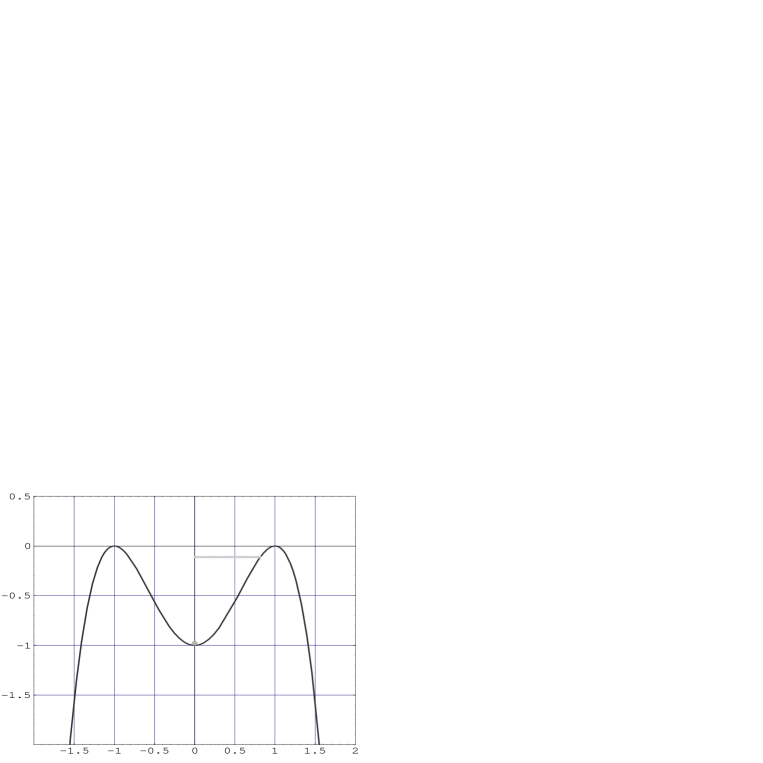
$\varphi^{\prime}$

FIG. 1.: The black line corresponds to the effective potential which determines $h(x_{5})$. The horizontal gray line represents a typical “energy” of $h(x_{5})$, the “trajectory” which minimizes the effective action $S$ of eq. (A4). The gray point, at $\left[\varphi^{\prime},{V(\varphi^{\prime})\over a^{2}}\right]=[0,-1]$, corresponds to the “static” solution.

REFERENCES

• [1] Q.R. Ahmad et al., SNO Collaboration, Phys. Rev. Lett. 87 (2001) 071301 [nucl-ex/0106015]; Phys. Rev. Lett. 89 (2002) 011301,2 [nucl-ex/0204008,9].
• [2] B.T. Cleveland et al., Astrophys. J. 496 (1998) 505; W. Hampel et al., GALLEX Collaboration, Phys. Lett. B 447 (1999) 127; J.N. Abdurashitov et al., SAGE Collaboration, Phys.  Rev. C 60 (1999) 055801 [astro-ph/9907113]; M. Altmann et al., GNO Collaboration, Phys.  Lett. B 490 (2000) 16 [hep-ex/0006034]; S. Fukuda et al., Super-Kamiokande Collaboration, Phys. Rev. Lett. 81 (1988) 4279; Phys. Rev. Lett. 86 (2001) 5651; M. Apollonio et al., CHOOZ Collaboration, Phys. Lett. B 466 (1999) 415 [hep-ex/9907037].
• [3] J.C. Pati and A. Salam, Phys. Rev. D 10 (1974) 275; R.N. Mohapatra and J.C. Pati, Phys. Rev. D 11 (1975) 566 and 2558; G. Senjanović and R.N. Mohapatra, Phys. Rev. D 12 (1975) 1502; G. Senjanović, Nucl. Phys. B 153 (1979) 334; R.N. Mohapatra and G. Senjanović, Phys. Rev. Lett. 44 (1980) 912; Phys. Rev. D 23 (1981) 165; C. S. Lim and T. Inami, Prog. Theor. Phys. 67 (1982) 1569.
• [4] T. G. Rizzo and G. Senjanović, Phys.  Rev.  Lett. 46 (1981) 1315; Phys.  Rev. D 24 (1981) 704; Phys. Rev. D 25 (1982) 235; M. Fukugita, T. Yanagida and M. Yoshimura, Phys.  Lett. B 106 (1981) 183; R. N. Mohapatra, Fortsch.  Phys. 31 (1983) 185.
• [5] I. Antoniadis, Phys. Lett. B 246 (1990) 377; N. Arkani-Hamed, S. Dimopoulos and G. Dvali, Phys. Lett. B 429 (1998) 263 [hep-ph/9803315]; I. Antoniadis, N. Arkani-Hamed, S. Dimopoulos and G. Dvali, Phys. Lett. B 436 (1998) 257 [hep-ph/9804398]; N. Arkani-Hamed and S. Dimopoulos, Phys. Rev.  D 65, (2002) 052003 [hep-ph/9811353]; Z. Berezhiani and Gia Dvali, Phys. Lett. B 450 (1999) 24 [hep-ph/9811378]; N. Arkani-Hamed, L. Hall, D. Smith and N. Weiner, Phys. Rev. D 61 (2000) 116003 [hep-ph/9909326].
• [6] C.D. Froggatt and H.B. Nielsen, Nucl. Phys. B 147 (1979) 277.
• [7] N. Arkani-Hamed and M. Schmaltz, Phys. Rev.  D 61 (2000) 033005 [hep-ph/9903417].
• [8] O. Khasanov and G. Perez, Phys. Rev. D 65 (2002) 053007 [hep-ph/0108176].
• [9] Y. Mimura and S. Nandi, hep-ph/0203126.
• [10] R. N. Mohapatra and A. Perez-Lorenzana, hep-ph/0205347.
• [11] D.E. Groom et. al., Eur. Phys. J. C 15 (2000) 1.
• [12] A. Bandyopadhyay, S. Choubey, S. Goswami and D.P. Roy hep-ph/0204286; J. N. Bahcall, M.C. Gonzalez-Garcia and C. Pena-Garay, hep-ph/0204314; V. Barger, D. Marfatia, K. Whisnant and B.P. Wood, Phys. Lett. B 537 (2002) [hep-ph/0204253]; G.L. Fogli, et. al, hep-ph/0206162; P.C. de Holanda and A.Y. Smirnov, hep-ph/0205241; C.V.K. Baba, D. Indumathi and M.V.N. Murthy, Phys. Rev. D 65 (2002) 073033, [hep-ph/0201031]; A. Strumia, C. Cattadori, N. Ferrari and F. Vissani, hep-ph/0205261; S.M. Bilenky, D. Nicolo and S.T. Petcov, Phys. Lett. B 538 (2002) 77 [hep-ph/0112216]; M.C. Gonzalez-Garcia, M. Maltoni, C. Pena-Garay and J.W  Valle, Phys. Rev. D 63 (2001) 033005 [hep-ph/0009350]; M. Maltoni, T. Schwetz, M.A. Tortola and J.W.F. Valle, hep-ph/0207227.
• [13] M.C. Gonzalez-Garcia and Y. Nir, hep-ph/0202058, to appear in Rev.  Mod.  Phys. .
• [14] L. Baudis et. al., Heidelberg-Moscow Double-Beta Decay Exp., Phys. Rev. Lett. 83 (1999) 41 [hep-ex/9902014]; H.V. Klapdor-Kleingrothaus et al., Heidelberg-Moscow Double-Beta Decay Exp., Nucl. Phys. A 694 (2001) 269.
• [15] S. Pascoli and S.T. Petcov, hep-ph/0205022.
• [16] S.S. Gershtein and Ya. B. Zeldovich, JETP   Lett. 4 (1966) 120; R. Cowsik and J. McClelland, Phys. Rev. Lett. 29 (1972) 669; J.R. Primack and M.A.K. Gross, astro-ph/0007165, to appear in Current Aspects of Neutrino Physics, ed. D. O. Caldwell (Springer, Berlin Heidelberg 2000); S. Hannestad, astro-ph/0205223.
• [17] J.F. Gunion, J. Grifols, A. Mendez, B. Kayser and F. Olness, Phys. Rev. D 40 (1989) 1546.
• [18] M. Gell-Mann, P. Ramond and R. Slansky, Supergravity, ed. P. van Niewenhuizen and D. Freedman (North-Holland 1979); T. Yanagida, Proceedings of the Workshop on the Unified Theory and the Baryon Number in the Universe, ed. O. Sawada and A. Sugamoto (Tsukuba 1979); R. N. Mohapatra and G. Senjanović, Phys. Rev. Lett. 44, 912 (1980).
• [19] H. Georgi, A.K. Grant and G. Hailu, Phys. Rev. D 63 (2001) 064027 [hep-ph/0007350].
• [20] K.R. Dienes, E. Dudas and T. Gherghetta, Nucl. Phys. B 537 (1999) 47 [hep-ph/9806292]; H.C. Cheng, B.A. Dobrescu and C.T. Hill, Nucl. Phys.  B 589 (2000) 249 [arXiv:hep-ph/9912343].
• [21] A. Aranda and J.L. Diaz-Cruz, hep-ph/0207059.
• [22] H. Georgi, A.K. Grant and G. Hailu, Phys. Lett.  B 506 (2001) 207 [hep-ph/0012379]; S. Nussinov and R. Shrock, Phys. Lett.  B 526 (2002) 137 [hep-ph/0101340].
• [23] N. Arkani-Hamed, A.G. Cohen and H. Georgi, Phys. Lett.  B 516 (2001) 395 [hep-th/0103135]; R. Barbieri, et. al, hep-th/0203039; C. Csaki, et. al, Phys.  Rev.  D 65 (2002) 085033 [hep-th/0203039]; W. Skiba and D. Smith, Phys. Rev. D 65 (2002) 095002 [hep-ph/0201056] ; E. Poppitz and Y. Shirman, hep-th/0204075.
• [24] D.E. Kaplan and T.M. Tait, JHEP 0111 (2001) 051 [hep-ph/0110126].
• [25] S.T. Petcov, Phys. Lett. B 110 (1982) 245.
• [26] R. Barbieri et. al., JHEP 12 (1998) 98017 [hep-ph/9807235].
• [27] Y. Kuno and Y. Okada, Rev.  Mod. Phys. 73 (2001) 151 [hep-ph/9909265].
• [28] S.M. Bilenky and S.T. Petcov Rev.  Mod. Phys. 59 (1987) 671.
• [29] R.N. Mohapatra and P.B. Pal, Massive Neutrinos in Physics and Astrophysics, World Scientific, Singapore (1991).
• [30] S.T. Petcov and A.Y. Smirnov, Phys. Lett. B 322 (1994) 109 [hep-ph/9311204]; S. Pascoli, S.T. Petcov and L. Wolfenstein, Phys. Lett. B 524 (2002) 319 [hep-ph/0110287]; G. Altarelli and F. Feruglio, Neutrino Mass, Springer Tracts in Modern Physics, ed. by G. Altarelli and K. Winter [hep-ph/0206077].
• [31] Y. Grossman and G. Perez, in preparation.
• [32] S. Coleman, Aspects of Symmetry, Cambridge University Press (1995).
• [33] I.S. Gradshteyn and I.M. Ryzhik, Tables of Integrals, Series, and Products, Fifth Ed., Academic Press, Inc. (1994).