Production of a pseudo-scalar Higgs boson at hadron colliders at next-to-next-to-leading order

Abstract:

The production cross section for pseudo-scalar Higgs bosons at hadron colliders is computed at next-to-next-to-leading order (NNLO) in QCD. The pseudo-scalar Higgs is assumed to couple only to top quarks. The NNLO effects are evaluated using an effective lagrangian where the top quarks are integrated out. The NNLO corrections are similar in size to those found for scalar Higgs boson production.

1 Introduction

In its minimal version, the Standard Model of particle interactions requires a complex scalar weak-isospin doublet to spontaneously break the electro-weak gauge symmetry. Three of its four original degrees of freedom transform into the longitudinal modes of the $W^{\pm}$ and $Z$ gauge bosons while the fourth manifests itself as a neutral scalar field, the Higgs boson. Yukawa-type couplings between the Higgs field and the fermions generate gauge invariant masses for the fermions.

There is no strong theoretical reason to believe that the minimal version of the Standard Model is indeed realized in nature. Extended models give rise to several Higgs particles which can be electrically charged or neutral and which can be even or odd under CP inversion.

The most appealing extension of the Standard Model, at the moment, is the Minimal Supersymmetric Standard Model (MSSM), which basically doubles the field content of the Standard Model and requires two Higgs doublets for the generation of the particle masses. This results in five physical Higgs bosons: three neutral ($h,H,A$) and two charged ($H^{\pm}$). $h$ and $H$ are CP-even while $A$ is CP-odd (for a review see Ref. [1]).

To date, no Higgs boson has been observed in nature, in spite of great efforts that have been made at particle accelerators, especially at the Large Electron Positron collider (LEP) at CERN. The null results lead to lower limits on the mass of possible Higgs bosons. For a scalar Higgs boson in the framework of the minimal Standard Model, this limit is $M_{H}\geq 114.4$ GeV at $95\%$ CL. Assuming the MSSM, the limit for a neutral scalar Higgs goes down to about 91 GeV. The $95\%$ CL limit on a CP-odd Higgs boson, the subject of this paper, is around 92 GeV [2].

The Large Hadron Collider (LHC) at CERN is scheduled to commence taking data in the year 2007. It will be a proton-proton collider with a center of mass energy of $\sqrt{s}=14$ TeV and has been designed specifically to search for Higgs bosons. For all relevant values of the Higgs boson mass and most kinds of Higgs bosons in various models, the gluon-gluon production mode will be of the greatest importance both for discovery and for measuring the Higgs boson mass. For CP-even Higgs bosons, the theoretical prediction is now fairly well under control, having been calculated to next-to-next-to-leading order (NNLO) in the strong coupling constant [3, 4].

In this paper, we use the techniques of Ref. [5, 3, 6] to evaluate the production rate for a pseudo-scalar Higgs boson to the same accuracy, i.e., to next-to-next-to-leading order in QCD. We work in the heavy-top limit, using an effective lagrangian for the interaction of the pseudo-scalar Higgs boson with the gluons. As in the case of the scalar Higgs boson, this does not restrict the validity of the results to the Higgs-mass region well below $2M_{t}$ if one factors in the full top mass dependence at leading order [7].

In the effective lagrangian approach, the massive top-quark loop that mediates the coupling between the Higgs and the constituents of the initial state hadrons, reduces to effective vertices with known coefficient functions. What remains to be computed at NNLO are $2\to 1$ processes up to two loops, $2\to 2$ up to one loop, and $2\to 3$ at tree level, where all internal particles are massless, and all external particles are taken on-shell ($p_{i}^{2}=0$ for quarks and gluons, $q^{2}=M_{A}^{2}$ for the Higgs).

We note that we do not consider contributions from virtual particles in extended theories in this paper. We also do not consider the effect of $b$ quark loops at this order, which can be important for example in the MSSM, when the coupling is enhanced by a large value of $\tan\beta$. For light quarks, like the $b$, the effective lagrangian cannot be formulated and one must perform a true three-loop calculation at this order. That calculation is beyond the current state of the art.

NLO corrections to this process were evaluated in Ref. [7, 8] and found to be very similar in size to the NLO effects for scalar Higgs production. We find that this is also true at NNLO: The K-factors at NNLO for the scalar and the pseudo-scalar are comparable. This means in turn that the production rate for pseudo-scalar Higgs bosons is fairly well under control. Though still sizable, the NNLO term in the perturbative series is significantly smaller than the NLO term and still higher order effects are presumably negligible. Accordingly, the unphysical dependence of the cross section on the renormalization and factorization scales is reasonably small, allowing for a prediction of the total rate with errors of the order of, or below, the expected experimental precision.

The paper is organized as follows: In the second section, we describe our theoretical framework, including the effective lagrangian, its Wilson coefficients and the renormalization of its operators, and our prescription for handling Levi-Civita tensors and $\gamma_{5}$. In the third section, we briefly discuss the matrix element calculations and the calculation of the partonic cross sections. In section 4, we present our results for the partonic cross sections. The result for pseudo-scalar production is very similar to that for scalar production and the expression for the difference between the two is quite compact. The full expression is presented in the appendix. In section 5 we compute the hadronic cross section by folding in the parton distributions and finally we present our conclusions.

2 Theoretical setup

In principle, the whole theoretical background is laid out very clearly in Ref. [9]. Nevertheless, let us review the necessary ingredients for our calculation.

We assume that the pseudo-scalar Higgs boson, $A$, couples only to top quarks, $t$. The interaction vertex is given by

$$\begin{split}{\cal L}_{At\bar{t}}=-ig_{t}\frac{A}{v}\,M_{t}\,\bar{t}\gamma_{5}t\,,\end{split}$$ (1)

where $g_{t}$ is a coupling constant that depends on the specific theory under consideration. In the MSSM, for example, one has $g_{t}=\cot\beta$, where $\tan\beta$ is the standard ratio of the vacuum expectation values of the two Higgs fields.

The coupling of $A$ to two gluons is then mediated by a top quark loop. In the heavy-top limit, this interaction can be described by an effective lagrangian [9]:

$$\begin{split}{\cal L}_{Agg}&=-g_{t}\,\frac{A}{v}\left[\tilde{C}_{1}^{\rm B}\,\tilde{\cal O}_{1}^{\rm B}+\tilde{C}^{\rm B}_{2}\,\tilde{\cal O}^{\rm B}_{2}\right]\,,\\ \tilde{\cal O}_{1}^{\rm B}&=G^{a}_{\mu\nu}\tilde{G}^{a,\mu\nu}\,,\qquad\tilde{\cal O}^{\rm B}_{2}=\partial_{\mu}\left(\sum_{q}\bar{q}\gamma^{\mu}\,\gamma_{5}q\right)\,.\end{split}$$ (2)

$G_{\mu\nu}^{a}$ is the gluon field strength tensor, and $\tilde{G}^{a}_{\mu\nu}$ is its dual:

$$\begin{split}\tilde{G}^{a}_{\mu\nu}=\epsilon_{\mu\nu\alpha\beta}\,G^{a,\alpha\beta}\,.\end{split}$$ (3)

All quantities in these equations are to be understood as bare quantities in the effective theory of five massless flavors. Thus the sum over quarks ($\sum_{q}$) in Eq. (2) does not include the top quark. $\tilde{C}_{1}^{\rm B}$ and $\tilde{C}^{\rm B}_{2}$ are coefficient functions that can be evaluated perturbatively. One may define renormalized operators and coefficient functions as follows:

$$\begin{split}\tilde{\cal O}_{i}=\sum_{j=1}^{2}Z_{ij}\tilde{\cal O}_{j}^{\rm B}\,,\qquad\tilde{C}_{i}=\sum_{j=1}^{2}(Z^{-1})_{ji}\tilde{C}_{j}^{\rm B}\,,\qquad i=1,2\,.\end{split}$$ (4)

The renormalization matrix $Z$ is given by [11]

$$\begin{split}Z_{11}&=Z_{\alpha_{s}}\,,\qquad Z_{12}=\frac{4}{\epsilon}\,\frac{\alpha_{s}}{\pi}+{\cal O}(\alpha_{s}^{2})\,,\\ Z_{21}&=0\,,\qquad\quad Z_{22}=Z_{\rm MS}^{s}\,Z_{5}^{s}\,,\end{split}$$ (5)

with

$$\begin{split}Z_{\alpha_{s}}&=1-\frac{\alpha_{s}}{\pi}\,\frac{\beta_{0}}{\epsilon}+\left(\frac{\alpha_{s}}{\pi}\right)^{2}\,\left(\frac{\beta_{0}^{2}}{\epsilon^{2}}-\frac{\beta_{1}}{2\epsilon}\right)+{\cal O}(\alpha_{s}^{3})\,,\\ \beta_{0}&=\frac{1}{4}\left(11-\frac{2}{3}n_{f}\right)\,,\qquad\beta_{1}=\frac{1}{16}\left(102-\frac{38}{3}n_{f}\right)\,,\\ Z_{\rm MS}^{s}&=1+\left(\frac{\alpha_{s}}{\pi}\right)^{2}\,\frac{1}{\epsilon}\,\left[\frac{11}{6}+\frac{5}{36}\,n_{f}\right]+{\cal O}(\alpha_{s}^{3})\,,\\ Z_{5}^{s}&=1-\frac{\alpha_{s}}{\pi}\,\frac{4}{3}+{\cal O}(\alpha_{s}^{2})\,,\end{split}$$ (6)

where $n_{f}$ is the number of light (i.e. massless in our approach) quark flavors. In our numerical analysis below, we will always assume $n_{f}=5$. $Z_{\alpha_{s}}$ and $Z_{\rm MS}^{s}$ are the renormalization constants of the strong coupling and the singlet axial current, respectively. $Z_{5}^{s}$ is a finite renormalization constant that will be discussed below.

The coefficient functions are process independent and have been evaluated in the context of pseudo-scalar Higgs decay to NNLO [9]:

$$\begin{split}\tilde{C}_{1}(\alpha_{s})&\equiv-\frac{\alpha_{s}}{\pi}\,\frac{1}{16}+{\cal O}(\alpha_{s}^{4})\,,\\ \tilde{C}_{2}(\alpha_{s})&=\left(\frac{\alpha_{s}}{\pi}\right)^{2}\,\left(\frac{1}{8}-\frac{1}{4}\,\ln\frac{\mu^{2}}{M_{t}^{2}}\right)+{\cal O}(\alpha_{s}^{3})\,,\end{split}$$ (7)

where $M_{t}$ is the pole mass of the top quark.

The matrix elements to be evaluated have the form

$$\begin{split}\langle\tilde{C}_{1}\tilde{\cal O}_{1}&+\tilde{C}_{2}\tilde{\cal O}_{2}\rangle=\tilde{C}_{1}Z_{11}\,\langle\tilde{\cal O}_{1}^{\rm B}\rangle+(\tilde{C}_{1}Z_{12}+\tilde{C}_{2}Z_{22})\,\langle\tilde{\cal O}_{2}^{\rm B}\rangle\,,\end{split}$$ (8)

with $\langle\tilde{\cal O}_{n}^{\rm B}\rangle\equiv\langle ab|\tilde{\cal O}_{n}^{\rm B}|XH\rangle$, where $a$ and $b$ label the two partons in the initial state, and $X$ denotes an arbitrary number of partons in the final state. We need to evaluate the square of this matrix element up to ${\cal O}(\alpha_{s}^{4})$.

$(a)$	$(b)$	$(c)$	$(d)$

Figure 1: Sample diagrams for $\langle\tilde{\cal O}_{1}^{\rm B}\rangle$. Higher orders are obtained by dressing these diagrams with additional quarks and gluons, both virtual and real.

$(a)$	$(b)$	$(c)$	$(d)$

Figure 2: Sample diagrams for $\langle\tilde{\cal O}_{2}^{\rm B}\rangle$ as required up to NNLO.

$\tilde{\cal O}_{1}^{\rm B}$ generates vertices which couple two or three gluons to the pseudo-scalar Higgs (the $ggggA$-vertex vanishes due to the Jacobi-identity of the structure functions of SU(3)). Thus, the diagrams related to $\langle\tilde{\cal O}_{1}^{\rm B}\rangle$ are the same as in the scalar Higgs case (cf. Ref. [10]). A sample of typical diagrams is shown in Fig. 1. Higher order contributions are obtained by dressing these diagrams with additional gluons and quarks, either as virtual particles, or as real particles in the final state. The actual results for these diagrams are different from the ones in the scalar case, of course, due to the different Feynman rules corresponding to $G_{\mu\nu}G^{\mu\nu}$ and $G_{\mu\nu}\tilde{G}^{\mu\nu}$.

As for $\langle\tilde{\cal O}_{2}^{\rm B}\rangle$, since its prefactor in Eq. (8) is of order $\alpha_{s}^{2}$, it is only required to one order less than $\langle\tilde{\cal O}_{1}^{\rm B}\rangle$. Diagrams contributing to $\langle\tilde{\cal O}_{2}^{\rm B}\rangle$ for the different subprocesses are shown in Fig. 2. They appear in interference terms with the corresponding diagrams of $\langle\tilde{\cal O}_{1}^{\rm B}\rangle$ (see Fig. 1). At NNLO, the square of diagram $(c)$ is the only potential contribution to the process arising solely through $\tilde{\cal O}_{2}^{\rm B}$. It vanishes, however, in the limit that the light quarks are massless.

When evaluating the diagrams, the presence of the manifestly 4-dimensional Levi-Civita tensor in $\tilde{\cal O}_{1}^{\rm B}$ as well as the $\gamma_{5}$ in $\tilde{\cal O}_{2}^{\rm B}$ requires special care. We strictly follow the strategy outlined in Ref. [11]. This means that first we replace

$$\begin{split}\lower 0.6458pt\hbox{/}\kern-5.00002pt\kern 0.08855pt\hbox{$q$}\kern 0.08855pt\gamma_{5}&\to\frac{i}{3!}q^{\alpha}\epsilon_{\alpha\beta\gamma\delta}\,\gamma^{\beta}\gamma^{\gamma}\gamma^{\delta}\,.\end{split}$$ (9)

Since we need to evaluate squared amplitudes, there will always be exactly two Levi-Civita tensors in our expressions. This allows us to express them in terms of metric tensors, which can be interpreted as $d$-dimensional objects:

$$\begin{split}\epsilon_{\alpha\beta\gamma\delta}\epsilon^{\bar{\alpha}\bar{\beta}\bar{\gamma}\bar{\delta}}=-g_{\alpha}^{[\bar{\alpha}}g_{\beta}^{\bar{\beta}}g_{\gamma}^{\bar{\gamma}}g_{\delta}^{\bar{\delta}]}=-g_{\alpha}^{\bar{\alpha}}g_{\beta}^{\bar{\beta}}g_{\gamma}^{\bar{\gamma}}g_{\delta}^{\bar{\delta}}+g_{\alpha}^{\bar{\beta}}g_{\beta}^{\bar{\alpha}}g_{\gamma}^{\bar{\gamma}}g_{\delta}^{\bar{\delta}}\mp\dots\,,\end{split}$$ (10)

where, as indicated, the brackets around the upper indices indicate that their positions are to be anti-symmetrized while the lower indices remain fixed. All further calculations (i.e., integrations, contraction of indices and spinor algebra) can be performed in $d$ dimensions. This procedure is slightly different from that of Ref. [9], but we have checked that it gives the same result for the pseudo-scalar Higgs decay up to ${\cal O}(\alpha_{s}^{4})$. Furthermore, we have computed the two-loop virtual corrections for our process in both approaches and obtained identical results.

The finite renormalization constant $Z^{s}_{5}$, introduced in Eq. (6), is determined by requiring that the one-loop character of the operator relation of the axial anomaly is preserved also at higher orders:

$$\begin{split}\tilde{\cal O}_{2}=\frac{\alpha_{s}}{\pi}\frac{n_{f}}{8}\,\tilde{\cal O}_{1}\,.\end{split}$$ (11)

Note that $\tilde{\cal O}_{1}$ and $\tilde{\cal O}_{2}$ denote renormalized operators here, as defined in Eq. (4).

3 Methods of evaluation

3.1 Virtual corrections

Potential sub-processes are $gg\to A$ and $q\bar{q}\to A$. It turns out, however, that the latter does not contribute at NNLO. The diagrams needed are two-loop vertices with one massive and two massless external legs.

For their evaluation, we use the technique of Ref. [12] that has already been applied successfully to the evaluation of the virtual correction to scalar Higgs production [5]. This means that the two-loop vertex diagrams are first mapped onto three-loop propagator diagrams by interpreting the massless external lines (gluons or quarks) as part of an additional loop. The resulting integrals, including tensor structures, can be treated by means of the integration-by-parts algorithm of Ref. [13]. In particular, we can use the FORM [14] program MINCER [15] as the basis of an algebraic program that reduces all integrals encountered to a set of master integrals [5]. The analytic expressions for the latter have been known for a long time [16]. Note that a generalized version of the method of Ref. [12] has been constructed in Ref. [4].

3.2 Single real emission

The radiation of one additional parton has to be evaluated up to one-loop level. The contributing processes are $gg\to Ag$, $gq\to Aq$, $g\bar{q}\to A\bar{q}$, and $q\bar{q}\to Ag$. The one-loop matrix elements have been evaluated to all orders in the dimensional regularization parameter $\epsilon=(4-d)/2$. After interfering with the tree-level amplitude, the squared matrix element can be integrated over single-emission phase space to obtain the contribution to the partonic cross section in closed analytic form. The interference of bare operators $\tilde{\cal O}_{1}^{\rm B}$ and $\tilde{\cal O}_{2}^{\rm B}$ is of order $\epsilon$. Nonetheless, operator $\tilde{\cal O}_{2}^{\rm B}$ contributes to the single real emission cross section through operator mixing since $Z_{12}$ is of order $1/\epsilon$. The Feynman rules, loop integrals and phase space integration have all been implemented in FORM programs.

3.3 Double real emission

We need the tree-level expressions for the processes $gg\to Agg$, $gg\to Aq\bar{q}$, $gq\to Agq$, $q\bar{q}\to Agg$, $q\bar{q}\to Aq\bar{q}$, and $qq\to Aqq$ (and the corresponding charged conjugated processes). The squared matrix elements can be evaluated straightforwardly in $d=4-2\epsilon$ space-time dimensions with the help of FORM. The result is a rather large expression of several thousand terms which must then be integrated over phase space.

The phase space for double real emission is quite complicated and we perform the integration in the method of Ref. [3]. That is, the matrix element and the phase space are expanded in terms of $(1-x)$, where $x=M_{A}^{2}/\hat{s}$. The result is a power series expansion in $(1-x)$ and $\ln(1-x)$ (at NNLO, the highest power of the logarithm is $\ln^{3}(1-x)$) for the double real emission contribution to the hadronic cross section. If one were to compute all terms in the series, this would be an exact result.

In fact, a truncated series is sufficient for obtaining the NNLO cross section to very high numerical precision. In this case, one obtains a cancellation of infrared singularities by expanding the other contributions to the partonic cross section (single real emission, mass factorization; the dependence of the virtual terms on $x$ is simply $\propto\delta(1-x)$) to the same order in $(1-x)$ as the double real emission term. In Ref. [3], we computed scalar Higgs boson production to order $(1-x)^{16}$ and arrived at a prediction for the hadronic cross section that is phenomenologically equivalent to one based on the closed analytic form of the partonic cross section that has recently become available [4]. This comes as no great surprise. The functions which contribute to the closed analytic form can all be expanded in terms of $(1-x)$. For example, the dilogarithm can be represented as

$$\begin{split}{\rm Li}_{2}(x)=\frac{\pi^{2}}{6}-\sum_{n=1}^{\infty}\frac{(1-x)^{n}}{n}\left(\frac{1}{n}-\ln(1-x)\right)\,.\end{split}$$ (12)

Furthermore, steeply falling parton distributions ensure that the threshold region dominates and that convergence in $(1-x)$ is quite rapid.

Although the truncated series leads to a physical result that is by all means equivalent to the exact expression, the approach of expanding in $(1-x)$ can be taken farther. If the expansion can be evaluated up to sufficiently high order in $(1-x)$, one can actually invert the series and obtain the partonic cross section in closed analytic form. This is due to the fact that only a limited number of functions appear in this closed form representation: logarithms, dilogarithms, and trilogarithms of various arguments, multiplied by $1/x$, $1/(1+x)$and $(1-x)^{n},n=-1,0,1,2,3$. Taking the functions which appear in the result for the Drell-Yan cross section [17] and these possible factors, one finds that carrying out the expansion to order $(1-x)^{96}$ should suffice to allow inversion of the series. In fact, we have carried out the expansion to order $(1-x)^{100}$ so that we could over-determine the system. As a check, this procedure has also been carried out for the scalar Higgs boson [6], and complete agreement with the result of Ref. [4] was found.

It is interesting to observe that the task of inverting the series is much simpler when one examines only the difference between the scalar and pseudo-scalar cases since they are already very similar at the level of squared amplitudes. The difference may be inverted with less than twenty terms.

4 Partonic results

As noted above, the partonic cross sections for scalar and pseudo-scalar Higgs production are very similar, so that many terms cancel in the difference between the two. Thus, the partonic cross section for pseudo-scalar Higgs production can be expressed conveniently in terms of the known scalar Higgs boson cross section (with modified normalization) plus a remainder. For this purpose, we write

$$\begin{split}\hat{\sigma}_{ab\Phi}&=\sigma^{0}_{\Phi}\,\Delta_{ab\Phi}\,,\qquad\Phi\in\{H,A\},\qquad a,b\in\{g,q,\bar{q}\}\,,\end{split}$$ (13)

where $\hat{\sigma}_{ab\Phi}$ is the cross section for the process $ab\to\Phi+X$. $a$ and $b$ label the partons in the initial state, $\Phi$ means either a scalar ($H$) or pseudo-scalar ($A$) Higgs boson, and $X$ denotes any number of quarks or gluons in the final state. In the normalization factors, we keep the full top mass dependence:

$$\begin{split}\sigma^{0}_{H}&=\frac{\pi\,\sqrt{2}\,G_{\rm F}}{256}\left(\frac{\alpha_{s}}{\pi}\right)^{2}\,\bigg{|}\tau_{H}\left[1+(1-\tau_{H})\,f(\tau_{H})\right]\bigg{|}^{2}\,,\\ \sigma^{0}_{A}&=\frac{\pi\,\sqrt{2}\,G_{\rm F}}{256}\left(\frac{\alpha_{s}}{\pi}\right)^{2}\,\Big{|}g_{t}\,\tau_{A}\,f(\tau_{A})\Big{|}^{2}\,,\qquad\qquad\tau_{\Phi}=\frac{4M_{t}^{2}}{M_{\Phi}^{2}}\,,\end{split}$$ (14)

where $G_{\rm F}\approx 1.664\times 10^{-5}\,{\rm GeV}^{-2}$, and $g_{t}$ has been introduced in Eq. (1). The one-loop function appearing in Eq. (14) is defined by

$$\begin{split}f(\tau)&=\left\{\begin{array}[]{ll}\arcsin^{2}\frac{1}{\sqrt{\tau}}\,,&\tau\geq 1\,,\\ -\frac{1}{4}\left[\ln\frac{1+\sqrt{1-\tau}}{1-\sqrt{1-\tau}}-i\pi\right]\,,&\tau<1\,.\end{array}\right.\end{split}$$ (15)

For completeness, we note that in the heavy-top limit, the normalization factors approach the values

$$\begin{split}\sigma_{H}^{0}\ &\stackrel{{\scriptstyle M_{t}\to\infty}}{{\longrightarrow}}\ \frac{\pi\,\sqrt{2}\,G_{\rm F}}{576}\,,\qquad\quad\sigma_{A}^{0}\ \stackrel{{\scriptstyle M_{t}\to\infty}}{{\longrightarrow}}\ \frac{\pi\,\sqrt{2}\,G_{\rm F}}{256}\,|g_{t}|^{2}\,.\end{split}$$ (16)

The kinematic terms are written as a perturbative expansion:

$$\begin{split}\Delta_{ab\Phi}(x)&=\delta_{ag}\delta_{bg}\,\delta(1-x)+\frac{\alpha_{s}}{\pi}\,\Delta_{ab\Phi}^{(1)}(x)+\left(\frac{\alpha_{s}}{\pi}\right)^{2}\,\Delta_{ab\Phi}^{(2)}(x)+{\cal O}(\alpha_{s}^{3})\,.\end{split}$$ (17)

The results for scalar Higgs production up to NNLO ($\Phi=H$) can be found in Refs. [10, 3, 4].

With the help of these expressions, the corresponding results for the pseudo-scalar Higgs production cross section can be written in a rather compact form. At NLO, the result has been evaluated some time ago [7, 8]:

$$\begin{split}\Delta_{abA}^{(1)}(x)&=\Delta_{abH}^{(1)}(x)+\frac{1}{2}\,\delta_{ag}\delta_{bg}\,\delta(1-x)\,,\qquad a,b\in\{g,q,\bar{q}\}\,.\end{split}$$ (18)

The main result of this paper are the NNLO terms in $\Delta_{abA}$. We find:

$$\begin{split}\Delta_{ggA}^{(2)}&(x)=\Delta_{ggH}^{(2)}(x)+\bigg{[}\frac{1939}{144}-\frac{19}{8}\,l_{Ht}+3\,\zeta_{2}\bigg{]}\,\delta(1-x)+6\,{\cal D}_{1}(x)\\ &-(12\,x-6\,x^{2}+6\,x^{3})\,\ln(1-x)-9\,x\,\ln^{2}(x)\\ &+\frac{3}{2}\,\frac{(10-x-13\,x^{2}+4\,x^{3}-2\,x^{4})}{1-x}\,\ln(x)+\frac{(154-189\,x+24\,x^{2}+11\,x^{3})}{4}\\ &+n_{f}\bigg{[}\left(-\frac{13}{16}-\frac{2}{3}\,l_{Ht}+2\,\delta_{2}\right)\,\delta(1-x)+\frac{2}{3}\,x\,\ln^{2}(x)+x\,\ln(x)\\ &\qquad-\frac{(1-11\,x+10\,x^{2})}{6}\bigg{]}\,,\quad\mbox{with}\qquad\delta_{2}=-\frac{1}{4}+\frac{1}{2}\,l_{Ht}\,,\\ \Delta_{gqA}^{(2)}&(x)=\Delta_{gqH}^{(2)}(x)+\frac{(4-4\,x+2\,x^{2})}{3}\ln(1-x)-\frac{28}{9}\,x\,\ln^{2}(x)\\ &+\frac{(22+30\,x-x^{2})}{3}\ln(x)+\frac{(337-382\,x+51\,x^{2})}{18}\,,\\ \Delta_{qqA}^{(2)}&(x)=\Delta_{qqH}^{(2)}(x)-\frac{64}{27}\,x\,\ln^{2}(x)+\frac{16}{27}\,(6+11\,x)\,\ln(x)+\frac{8}{27}\,(37-40\,x+3\,x^{2})\,,\\ \Delta_{q\bar{q}A}^{(2)}&(x)=\Delta_{q\bar{q}H}^{(2)}(x)+\frac{32}{27}\,x\,\ln^{2}(x)+\frac{32}{27}\,(3+8\,x)\,\ln(x)\\ &+\frac{16}{27}\,(11-x-9\,x^{2}-x^{3})+n_{f}\,\bigg{[}-\frac{32}{27}\,x\,\ln(x)-\frac{16}{27}\,(1-x^{2})\bigg{]}\,,\\ \Delta_{qq^{\prime}A}^{(2)}&(x)=\Delta_{qq^{\prime}H}^{(2)}(x)-\frac{16}{9}\,x\,\ln^{2}(x)+\frac{16}{9}\,(2+3\,x)\,\ln(x)+\frac{8}{9}\,(11-12\,x+x^{2})\,,\end{split}$$ (19)

where $l_{Ht}\equiv\ln(M_{A}^{2}/M_{t}^{2})$, $\zeta_{n}\equiv\zeta(n)$ is Riemann’s $\zeta$ function ($\zeta_{2}=\pi^{2}/6=1.64483\ldots$, $\zeta_{3}=1.20206\ldots$) and ${\cal D}_{n}(x)\equiv[\ln^{n}(1-x)/(1-x)]_{+}$. Of course one must change $M_{H}\to M_{A}$ wherever it appears in $\Delta_{abH}$. For the sake of completeness, we list the full result for $\Delta_{abA}$ in App. A. The difference $\Delta_{abA}-\Delta_{abH}$ can be expanded readily in terms of $(1-x)$ in order to bring it to a form consistent with the results of Ref. [3].

The only contribution that originates from the presence of the (renormalized!) operator $\tilde{\cal O}_{2}$ is the term $\delta_{2}$ in the equations above. We obtain it by computing the interference of diagram $(a)$ in Fig. 1 with diagram $(a)$ of Fig. 2. Alternatively, it can be derived from Eq. (11) by using the LO result for $\Delta_{ggA}$:

$$\begin{split}(\tilde{C}_{1}\tilde{C}_{2})^{-1}\,n_{f}\,\delta_{2}\,\left(\frac{\alpha_{s}}{\pi}\right)^{4}\,\delta(1-x)&=\frac{\alpha_{s}}{\pi}\,\frac{n_{f}}{8}\left[\tilde{C}_{1}^{-2}\left(\frac{\alpha_{s}}{\pi}\right)^{2}\,\delta(1-x)\right]\,,\end{split}$$ (20)

which leads to the same result for $\delta_{2}$ as above. This provides a welcome check on the normalization of the contribution from $\tilde{\cal O}_{2}$.

5 Hadronic results

In complete analogy to scalar Higgs production, one has to convolute the partonic rate with the proper parton distribution functions, in order to arrive at a physical prediction for the hadronic production rate:

$$\begin{split}\sigma_{h_{1}h_{2}}(s)&=\sum_{a,b}\,\int_{0}^{1}\!d\tau\!\int_{\tau}^{1}\frac{dx_{a}}{x_{a}}\left[f_{a/h_{1}}(x_{a})\,f_{b/h_{2}}(\tau/x_{a})\right]\,{\hat{\sigma}}_{ab}(\hat{s}=s\tau).\end{split}$$ (21)

A consistent NNLO hadronic result requires not only a NNLO partonic cross section, but also PDFs that have been evaluated at NNLO. Strictly speaking, such a set of PDFs is not yet available, because the NNLO evolution equation is not fully known. Nevertheless, we use an approximate set of PDFs [18], based on approximations to the evolution equation [19] derived from the available moments of the structure functions [20]. At lower order, we use the corresponding lower order PDFs [21].

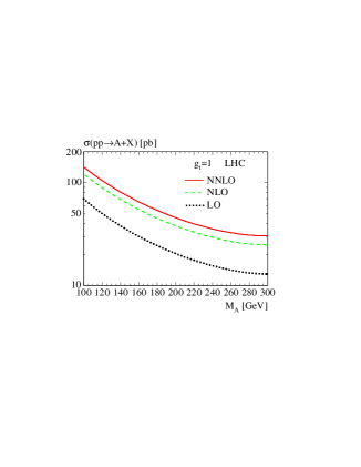
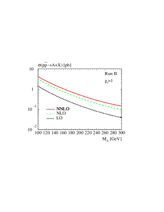
$(a)$	$(b)$

Figure 3: Total cross section for inclusive production of pseudo-scalar Higgs bosons ($A$) at $(a)$ the LHC ($\sqrt{s}=14$ TeV) and $(b)$ Tevatron Run II ($\sqrt{s}=2$ TeV). The coupling constant for the coupling of $A$ to top quarks is such that $g_{t}=1$. The cross section for other values of $g_{t}$ (e.g., $g_{t}=\cot\beta$ in the MSSM) can be obtained by scaling the curves with $|g_{t}|^{2}$.

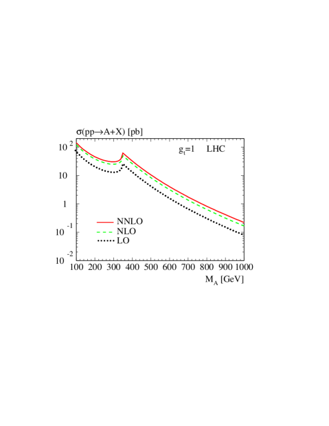
Figure 4: Total cross section for inclusive production of pseudo-scalar Higgs bosons ($A$) at the LHC ($\sqrt{s}=14$ TeV), as in Fig. 3 for a larger mass range. The cusp is an effect of the top-quark threshold.

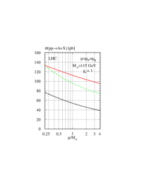
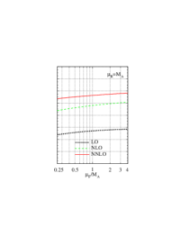
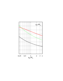
$(a)$	$(b)$	$(c)$

Figure 5: Scale dependence of the cross section for an $M_{A}=115$ GeV pseudo-scalar Higgs boson at the LHC ($\sqrt{s}=14$ TeV) $(a)$ varying $\mu_{F}=\mu_{R}$, $(b)$ varying $\mu_{F}$, $\mu_{R}=M_{A}$ and $(c)$ varying $\mu_{R}$, $\mu_{F}=M_{A}$.

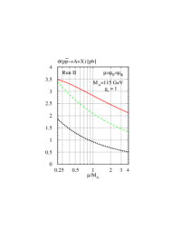
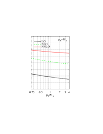
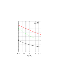
$(a)$	$(b)$	$(c)$

Figure 6: Same as Fig. 5 for the Tevatron Run II ($\sqrt{s}=2$ TeV).

Fig. 3 shows the total cross section as a function of the pseudo-scalar Higgs boson mass, $M_{A}$, at $(a)$ the LHC, and $(b)$ Tevatron Run II. Fig. 4 shows the curves for the LHC over a larger mass range. The renormalization and factorization scales have been set to $M_{A}$. The cusp in Fig. 4 is a leading order effect caused by the $t\bar{t}$ threshold, cf. Eq. (14). Since we do not want to specify a particular extension of the Standard Model, we choose the coupling of the pseudo-scalar Higgs to the top quarks such that $g_{t}=1$ (cf. Eq. (1)). The total cross section scales with $|g_{t}|^{2}$, so that the actual numbers can be easily obtained from the ones shown in the figure. As already noted, the behavior of the corrections is very similar to the ones for scalar Higgs production: The NNLO corrections are significantly smaller than the NLO corrections, indicating a nicely converging result with uncertainties well under control.

This is further affirmed in Figs. 5 and 6, which show the variation of the cross section with the renormalization and factorization scales for a fixed Higgs mass $M_{A}=115$ GeV. The scales are varied between $M_{A}/4$ and $4M_{A}$: in sub-panels $(a)$, the renormalization scale and the factorization scale are identified and varied simultaneously; in sub-panels $(b)$, the renormalization scale $\mu_{R}$ is identified with $M_{A}$, and $\mu_{F}$ is varied, while in sub-panels $(c)$, $\mu_{F}=M_{A}$ is fixed and $\mu_{R}$ is varied. One observes a clear reduction of the scale dependence at NNLO with respect to NLO. Compared to the LO curve, there is a significant relative improvement in the scale variation, while the absolute ranges of variation at LO and NNLO are comparable. It is also clear that the scale dependence is dominated by renormalization scale dependence; factorization scale dependence is quite small. Using the rather conservative range of $M_{A}/4<\mu<4M_{A}$, one arrives at an uncertainty in $\sigma$ from scale variation of about $\pm 30\%$ ($\pm 65\%$) at LO, $\pm 30\%$ ($\pm 50\%$) NLO, and less than $\pm 20\%$ ($\pm 25\%$) at NNLO for the LHC (numbers in brackets for Tevatron Run II). Varying $\mu$ between $M_{A}/2$ and $2M_{A}$ results in a variation of $\sigma$ of $\pm 20\%$ ($\pm 40\%$) at LO, $\pm 15\%$ ($\pm 25\%$) at NLO, and less than $\pm 10\%$ ($\pm 15\%$) at NNLO.

6 Conclusions

The hadronic cross section for the production of a pseudo-scalar Higgs boson has been calculated at NNLO in QCD. We find that the corrections are similar to the scalar case, both in their magnitude and in their uncertainty due to scale dependence. While this uncertainty is still rather large, it seems that the NNLO calculation yields a reliable prediction for the total rate.

Note Added:

As we completed this manuscript, we became aware of a similar paper by Anastasiou and Melnikov[22]. We have compared results for the partonic cross sections and find complete agreement.

Acknowledgments.

R.V.H. thanks the High Energy Theory group at Brookhaven National Laboratory, where part of this work has been done, for hospitality. The work of W.B.K. was supported by the U.S. Department of Energy under Contract No. DE-AC02-98CH10886.

Appendix A Analytic results

In this appendix, the analytic expressions for the partonic cross section of pseudo-scalar Higgs production at NNLO are listed. Note that using the formulas of Eqs. (18) and (19), one can transform these expressions into the corresponding ones for scalar Higgs production.

At NLO [7, 8], the result for the gluon-gluon sub-process is

$$\begin{split}\Delta_{ggA}^{(1)}(x)&=(6+6\,\zeta_{2})\,\delta(1-x)+12\,{\cal D}_{1}(x)-(24\,x-12\,x^{2}+12\,x^{3})\,\ln(1-x)\\ &-6\frac{(1-x+x^{2})^{2}}{1-x}\ln(x)-\frac{11}{2}(1-x)^{3}\,.\end{split}$$ (22)

For the quark-gluon channel one finds

$$\begin{split}\Delta_{gqA}^{(1)}(x)&=\frac{(8-8\,x+4\,x^{2})}{3}\ln(1-x)-\frac{(4-4\,x+2\,x^{2})}{3}\ln(x)-\frac{(3-6\,x+x^{2})}{3}\,,\end{split}$$ (23)

and for the quark–anti-quark channel

$$\begin{split}\Delta_{q\bar{q}A}^{(1)}(x)=&\frac{32}{27}(1-x)^{3}\,.\end{split}$$ (24)

The contributions from different sub-processes at NNLO are written as

$$\begin{split}\Delta_{abA}^{(2)}&=\Delta_{abA}^{A}+n_{f}\,\Delta_{abA}^{F}\,,\end{split}$$ (25)

where $n_{f}$ is the number of light (i.e., massless in our approach) quark flavors.

For the sub-process with two gluons in the initial state, we find

$$\begin{split}&\Delta_{ggA}^{A}(x)=\left[\frac{741}{8}+\frac{139}{2}\zeta_{2}-\frac{165}{4}\zeta_{3}-\frac{9}{20}\zeta_{2}^{2}\right]\delta(1-x)\\ &-\left[\frac{101}{3}-33\,\zeta_{2}-\frac{351}{2}\,\zeta_{3}\right]{\cal D}_{0}(x)+\left[139-90\,\zeta_{2}\right]{\cal D}_{1}(x)-33\,{\cal D}_{2}(x)+72\,{\cal D}_{3}(x)\\ &-(144\,x-72\,x^{2}+72\,x^{3})\ln^{3}(1-x)-(297-381\,x+348\,x^{2}-330\,x^{3})\ln^{2}(1-x)\\ &-\frac{9}{2}\,\frac{(31-30\,x+93\,x^{2}-94\,x^{3}+31\,x^{4})}{1-x}\ln^{2}(1-x)\ln(x)\\ &+\left[\frac{(2027-2735\,x+2182\,x^{2}-2583\,x^{3})}{4}+(180\,x-90\,x^{2}+90\,x^{3})\zeta_{2}\right]\ln(1-x)\\ &+3\,\frac{(88-211\,x+312\,x^{2}-365\,x^{3}+187\,x^{4})}{1-x}\ln(1-x)\ln(x)\\ &+9\,\frac{(7+3\,x+19\,x^{2}-3\,x^{3}-19\,x^{4}+9\,x^{5})}{1-x^{2}}\ln(1-x)\ln^{2}(x)\\ &+36\frac{(1-6\,x-13\,x^{2}-6\,x^{3}+x^{4})}{1+x}\ln(1-x){\rm Li}_{2}(1-x)\\ &-18\frac{(1+2\,x+3\,x^{2}+2\,x^{3}+x^{4})}{1+x}\ln(1-x){\rm Li}_{2}(1-x^{2})\\ &-\frac{9}{2}\frac{(24-38\,x+8\,x^{2}+54\,x^{3}-19\,x^{4}+9\,x^{5})}{1-x^{2}}{\rm Li}_{3}(1-x)\\ &-\frac{9}{2}\frac{(27+35\,x+75\,x^{2}-29\,x^{3}-78\,x^{4}+6\,x^{5})}{1-x^{2}}{\rm Li}_{3}\left(-\frac{(1-x)}{x}\right)\\ &+\frac{9}{8}\frac{(1+2\,x+3\,x^{2}+24\,x^{3}+16\,x^{4})}{1+x}{\rm Li}_{3}(1-x^{2})\\ &-\frac{9}{8}\frac{(1+2\,x+3\,x^{2}-8\,x^{3}-8\,x^{4})}{1+x}{\rm Li}_{3}\left(-\frac{(1-x^{2})}{x^{2}}\right)\\ &-\frac{9}{2}\frac{(7+14\,x+21\,x^{2}+8\,x^{3}+4\,x^{4})}{1+x}\left[{\rm Li}_{3}\left(\frac{1-x}{1+x}\right)-{\rm Li}_{3}\left(-\frac{1-x}{1+x}\right)\right]\\ &-\frac{3}{4}\frac{(317-398\,x-87\,x^{2}+300\,x^{3}-121\,x^{4})}{1-x}{\rm Li}_{2}(1-x)\\ &+\frac{9}{2}\frac{(11+31\,x+59\,x^{2}-25\,x^{3}-65\,x^{4}+11\,x^{5})}{1-x^{2}}{\rm Li}_{2}(1-x)\ln(x)\\ &+\frac{(42+36\,x-63\,x^{2}-33\,x^{3})}{4}{\rm Li}_{2}(1-x^{2})+\frac{9}{4}\frac{(5+10\,x+15\,x^{2}-2\,x^{4})}{1+x}{\rm Li}_{2}(1-x^{2})\ln(x)\\ &+\frac{3}{4}\frac{(21+23\,x+41\,x^{2}-37\,x^{3}-44\,x^{4}+4\,x^{5})}{1-x^{2}}\ln^{3}(x)\\ &-\frac{3}{8}\frac{(154-365\,x+675\,x^{2}-827\,x^{3}+374\,x^{4})}{1-x}\ln^{2}(x)\\ &-\frac{1}{8}\frac{(2213-5599\,x+6603\,x^{2}-7003\,x^{3}+4342\,x^{4})}{1-x}\ln(x)\\ &+9\,\frac{(9-2\,x+27\,x^{2}-34\,x^{3}+9\,x^{4})}{1-x}\zeta_{2}\,\ln(x)-\frac{(16309-20611\,x+23819\,x^{2}-22749\,x^{3})}{48}\\ &+\frac{3}{4}\,(319-277\,x+233\,x^{2}-363\,x^{3})\zeta_{2}-\frac{351}{2}\,\,(2\,x-x^{2}+x^{3})\zeta_{3}\end{split}$$ (26)

and

$$\begin{split}&\Delta_{ggA}^{F}(x)=\left[-\frac{689}{72}+l_{Ht}-\frac{5}{3}\,\zeta_{2}+\frac{5}{6}\,\zeta_{3}\right]\,\delta(1-x)\\ &+\left[\frac{14}{9}-2\,\zeta_{2}\right]\,{\cal D}_{0}(x)-\frac{10}{3}\,{\cal D}_{1}(x)+2\,{\cal D}_{2}(x)\\ &+\frac{2}{9}(8-12\,x+3\,x^{2}-17\,x^{3})\ln^{2}(1-x)+\frac{8}{3}(x+x^{2})\ln^{2}(1-x)\ln(x)\\ &-\frac{(922-294\,x+249\,x^{2}-1570\,x^{3})}{108}\ln(1-x)\\ &-\frac{2}{9}\frac{(17+7\,x+21\,x^{2}-61\,x^{3}+25\,x^{4})}{1-x}\ln(1-x)\ln(x)\\ &-\frac{8}{3}(x+x^{2})\ln^{2}(x)\ln(1-x)+\frac{16}{3}(x+x^{2})\ln(1-x)\,{\rm Li}_{2}(1-x)\\ &-\frac{(2+14\,x+17\,x^{2})}{6}{\rm Li}_{3}(1-x)-\frac{(2-34\,x-31\,x^{2})}{12}{\rm Li}_{3}\left(-\frac{(1-x)}{x}\right)\,.\\ &+\frac{1}{36}\frac{(68-302\,x+21\,x^{2}+227\,x^{3}+4\,x^{4})}{1-x}{\rm Li}_{2}(1-x)\\ &+\frac{(2-50\,x-47\,x^{2})}{12}{\rm Li}_{2}(1-x)\ln(x)\\ &+\frac{(2+6\,x+9\,x^{2})}{72}\ln^{3}(x)+\frac{1}{72}\frac{(68+100\,x+69\,x^{2}-351\,x^{3}+132\,x^{4})}{1-x}\ln^{2}(x)\\ &+\frac{1}{216}\frac{(1282-382\,x+117\,x^{2}-3041\,x^{3}+2384\,x^{4})}{1-x}\ln(x)-\frac{8}{3}(x+x^{2})\zeta_{2}\,\ln(x)\\ &+\frac{(12707-606\,x+1641\,x^{2}-17774\,x^{3})}{1296}-\frac{2}{9}(8-12\,x+3\,x^{2}-17\,x^{3})\,\zeta_{2}\end{split}$$ (27)

For the quark-gluon channel, we have:

$$\begin{split}&\Delta_{gqA}^{A}(x)=\frac{367}{54}(2-2\,x+x^{2})\ln^{3}(1-x)\\ &-\frac{(2592-2278\,x-111\,x^{2}-288\,x^{3})}{36}\ln^{2}(1-x)-\frac{(642+190\,x+553\,x^{2})}{18}\ln^{2}(1-x)\ln(x)\\ &+\left[\frac{(23887-17388\,x-2538\,x^{2}-784\,x^{3})}{162}-\frac{50}{9}(2-2\,x+x^{2})\zeta_{2}\,\right]\ln(1-x)\\ &+\frac{(1665-2040\,x+174\,x^{2}-400\,x^{3})}{27}\ln(1-x)\ln(x)\!+\frac{4(38+21\,x+39\,x^{2})}{9}\ln(1-x)\ln^{2}(x)\\ &-\frac{2}{9}(46+298\,x+139\,x^{2})\ln(1-x)\,{\rm Li}_{2}(1-x)-2(2+2\,x+x^{2})\ln(1-x)\,{\rm Li}_{2}(1-x^{2})\\ &-\frac{2}{9}(42-142\,x-x^{2}){\rm Li}_{3}(1-x)-\frac{(302+474\,x+339\,x^{2})}{9}{\rm Li}_{3}\left(-\frac{(1-x)}{x}\right)\\ &-\frac{(2+2\,x+x^{2})}{2}{\rm Li}_{3}(1-x^{2})-\frac{(2+2\,x+x^{2})}{2}{\rm Li}_{3}\left(-\frac{(1-x^{2})}{x^{2}}\right)\\ &-4(2+2\,x+x^{2})\left[{\rm Li}_{3}\left(\frac{1-x}{1+x}\right)-{\rm Li}_{3}\left(-\frac{1-x}{1+x}\right)\right]\\ &-\frac{(979-144\,x-215\,x^{2}+52\,x^{3})}{18}{\rm Li}_{2}(1-x)+\frac{(142+374\,x+245\,x^{2})}{9}{\rm Li}_{2}(1-x)\ln(x)\\ &+\frac{(166+222\,x+33\,x^{2}+4\,x^{3})}{54}{\rm Li}_{2}(1-x^{2})+2(2+2\,x+x^{2})\ln(x)\,{\rm Li}_{2}(1-x^{2})\\ &+\frac{(133+202\,x+115\,x^{2})}{27}\ln^{3}(x)-\frac{(837-1296\,x+234\,x^{2}-226\,x^{3})}{54}\ln^{2}(x)\\ &-\left[\frac{(22042-32040\,x-5847\,x^{2}-2464\,x^{3})}{324}-\frac{(194+222\,x+213\,x^{2})}{9}\zeta_{2}\right]\ln(x)\\ &-\frac{(173719-156324\,x-12687\,x^{2}-6148\,x^{3})}{1944}+\frac{(1071-710\,x-130\,x^{2}-144\,x^{3})}{18}\,\zeta_{2}\\ &+\frac{311}{18}(2-2\,x+x^{2})\,\zeta_{3}\end{split}$$ (28)

and

$$\begin{split}&\Delta_{gqA}^{F}(x)=\frac{(2-2\,x+x^{2})}{18}\ln^{2}(1-x)\\ &-\frac{(13-16\,x+9\,x^{2})}{9}\ln(1-x)-\frac{(4-4\,x+2\,x^{2})}{9}\ln(1-x)\ln(x)\\ &+\frac{(2-2\,x+x^{2})}{9}\ln^{2}(x)+\frac{(29-38\,x+19\,x^{2})}{27}\ln(x)+\frac{(265-418\,x+179\,x^{2})}{162}\,.\end{split}$$ (29)

For the scattering of two identical quarks, we find

$$\begin{split}\Delta_{qqA}^{A}&(x)=-\frac{32}{9}(3-2\,x-x^{2})\ln^{2}(1-x)-\frac{16}{9}(4+4\,x+x^{2})\ln^{2}(1-x)\ln(x)\\ &+\frac{4}{3}(17-12\,x-5\,x^{2})\ln(1-x)+\frac{8}{9}(12-8\,x-5\,x^{2})\ln(1-x)\ln(x)\\ &+\frac{8}{9}(4+4\,x+x^{2})\ln(1-x)\ln^{2}(x)-\frac{32}{9}(4+4\,x+x^{2})\ln(1-x){\rm Li}_{2}(1-x)\\ &-\frac{8}{27}(2-2\,x+x^{2}){\rm Li}_{3}(1-x)-\frac{8}{27}(50+46\,x+13\,x^{2}){\rm Li}_{3}\left(-\frac{(1-x)}{x}\right)\\ &-\frac{8}{9}(6-4\,x-x^{2}){\rm Li}_{2}(1-x)+\frac{16}{27}(19+17\,x+5\,x^{2}){\rm Li}_{2}(1-x)\ln(x)\\ &+\frac{8}{81}(19+17\,x+5\,x^{2})\ln^{3}(x)-\frac{4}{27}(18-10\,x-9\,x^{2})\ln^{2}(x)\\ &-\frac{2}{27}(129-212\,x-69\,x^{2})\ln(x)+\frac{16}{9}(4+4\,x+x^{2})\zeta_{2}\ln(x)\\ &+\frac{4}{27}(-86+53\,x+33\,x^{2})+\frac{32}{9}(3-2\,x-x^{2})\,\zeta_{2}\end{split}$$ (30)

and

$$\begin{split}\Delta_{qqA}^{F}&(x)=0\,.\end{split}$$ (31)

For the scattering of a quark–(anti-)quark pair of distinct flavor, we find

$$\begin{split}\Delta_{qq^{\prime}A}^{A}&(x)=-\frac{32}{9}(3-2\,x-x^{2})\ln^{2}(1-x)-\frac{16}{9}(4+4\,x+x^{2})\ln^{2}(1-x)\ln(x)\\ &+\frac{4}{3}(17-12\,x-5\,x^{2})\ln(1-x)+\frac{8}{9}(12-8\,x-5\,x^{2})\ln(1-x)\ln(x)\\ &+\frac{8}{9}(4+4\,x+x^{2})\ln(1-x)\ln^{2}(x)-\frac{32}{9}(4+4\,x+x^{2})\ln(1-x){\rm Li}_{2}(1-x)\\ &-\frac{32}{9}(4+4\,x+x^{2}){\rm Li}_{3}\left(-\frac{(1-x)}{x}\right)\\ &-\frac{8}{9}(6-4\,x-x^{2}){\rm Li}_{2}(1-x)+\frac{8}{3}(4+4\,x+x^{2}){\rm Li}_{2}(1-x)\ln(x)\\ &+\frac{4}{9}(4+4\,x+x^{2})\ln^{3}(x)-\frac{8}{9}(3-2\,x-x^{2})\ln^{2}(x)\\ &-\frac{2}{9}(43-68\,x-29\,x^{2})\ln(x)+\frac{16}{9}(4+4\,x+x^{2})\zeta_{2}\,\ln(x)\\ &-\frac{2}{9}(61-46\,x-15\,x^{2})+\frac{32}{9}(3-2\,x-x^{2})\,\zeta_{2}\end{split}$$ (32)

and

$$\begin{split}\Delta_{qq^{\prime}A}^{F}&(x)=0\,.\end{split}$$ (33)

For quark–anti-quark scattering (same quark flavor), we have

$$\begin{split}\Delta_{q\bar{q}A}^{A}&(x)=-\frac{32}{81}(14+21\,x-48\,x^{2}+13\,x^{3})\ln^{2}(1-x)-\frac{16}{9}(4+4\,x+x^{2})\ln^{2}(1-x)\ln(x)\\ &+\frac{4}{81}(75+892\,x-1351\,x^{2}+384\,x^{3})\ln(1-x)\\ &+\frac{8}{81}(76+72\,x-189\,x^{2}+64\,x^{3})\ln(1-x)\ln(x)\\ &+\frac{8}{9}(4+4\,x+x^{2})\ln(1-x)\ln^{2}(x)-\frac{32}{9}(4+4\,x+x^{2})\ln(1-x){\rm Li}_{2}(1-x)\\ &-\frac{40}{27}(2+2\,x+x^{2}){\rm Li}_{3}(1-x)-\frac{8}{9}(18+18\,x+5\,x^{2}){\rm Li}_{3}\left(-\frac{(1-x)}{x}\right)\\ &+\frac{10}{27}(2+2\,x+x^{2}){\rm Li}_{3}(1-x^{2})+\frac{2}{9}(2+2\,x+x^{2}){\rm Li}_{3}\left(-\frac{(1-x^{2})}{x^{2}}\right)\\ &+\frac{8}{27}(2+2\,x+x^{2})\left[{\rm Li}_{3}\left(\frac{1-x}{1+x}\right)-{\rm Li}_{3}\left(-\frac{1-x}{1+x}\right)\right]\\ &-\frac{8}{81}(12+30\,x-93\,x^{2}-26\,x^{3}){\rm Li}_{2}(1-x)+\frac{16}{9}(7+7\,x+2\,x^{2}){\rm Li}_{2}(1-x)\ln(x)\\ &-\frac{8}{27}\,(2\,x+x^{2}+6\,x^{3}){\rm Li}_{2}(1-x^{2})-\frac{4}{9}(2+2\,x+x^{2}){\rm Li}_{2}(1-x^{2})\ln(x)\\ &+\frac{8}{27}(5+5\,x+x^{2})\ln^{3}(x)-\frac{8}{81}(27+27\,x-81\,x^{2}+44\,x^{3})\ln^{2}(x)\\ &+\frac{2}{81}(9-1064\,x+2111\,x^{2}-768\,x^{3})\ln(x)+\frac{16}{9}(4+4\,x+x^{2})\zeta_{2}\,\ln(x)\\ &+\frac{20}{81}(101-462\,x+520\,x^{2}-159\,x^{3})+\frac{16}{81}(11+93\,x-147\,x^{2}+43\,x^{3})\,\zeta_{2}\end{split}$$ (34)

and

$$\begin{split}\Delta_{q\bar{q}A}^{F}&(x)=\frac{32(1-x)^{3}}{81}\ln(1-x)-\frac{16(3-9\,x+12\,x^{2}-4\,x^{3})}{81}\ln(x)\\ &-\frac{8(41-111\,x+111\,x^{2}-41\,x^{3})}{243}\,.\end{split}$$ (35)

In the expressions above, we have identified the renormalization and the factorization scale with the Higgs boson mass, $\mu_{R}=\mu_{F}=M_{A}$. The dependence on these scales is logarithmic and can readily be reconstructed by employing scale invariance of the total partonic cross section.

References

- [1] J.F. Gunion, H.E. Haber, G.L. Kane, S. Dawson, The Higgs Hunter’s Guide, Addison-Wesley, Reading 1990.
-
[2]
See
http://lephiggs.web.cern.ch/LEPHIGGS/www/Welcome.htmlfor updates. - [3] R.V. Harlander, W.B. Kilgore, Phys. Rev. Lett. 88 (2002) 201801.
- [4] C. Anastasiou, K. Melnikov, hep-ph/0207004.
- [5] R.V. Harlander, Phys. Lett. B 492 (2000) 74.
- [6] W.B. Kilgore, proceedings of the International Conference on High Energy Physics (ICHEP’02), Amsterdam, July 24-31, 2002 [hep-ph/0208143].
- [7] M. Spira, A. Djouadi, D. Graudenz, P.M. Zerwas, Nucl. Phys. B 453 (1995) 17; Phys. Lett. B 318 (1993) 347.
- [8] R.P. Kauffman, W. Schaffer, Phys. Rev. D 49 (1994) 551.
- [9] K.G. Chetyrkin, B.A. Kniehl, M. Steinhauser, W.A. Bardeen, Nucl. Phys. B 535 (1998) 3.
-
[10]
R.V. Harlander, W.B. Kilgore, Phys. Rev. D 64 (2001) 013015;
S. Catani,D. de Florian, M. Grazzini, J. High Energy Phys. 05 (2001) 025 - [11] S.A. Larin, he-ph/9302240; Phys. Lett. B 303 (1993) 113.
- [12] P.A. Baikov, V.A. Smirnov, Phys. Lett. B 477 (2000) 367.
-
[13]
F.V. Tkachov, Phys. Lett. B 100 (1981) 65;
K.G. Chetyrkin, F.V. Tkachov, Nucl. Phys. B 192 (1981) 159. - [14] J.A.M. Vermaseren, math-ph/0010025.
-
[15]
S.A. Larin, F.V. Tkachov, J.A.M. Vermaseren,
NIKHEF-H/91-18, Amsterdam, 1991 (see also
http://www.nikhef.nl/~form/). -
[16]
R.J. Gonsalves, Phys. Rev. D 28 (1983) 1542;
G. Kramer, B. Lampe, Z. Phys. C 34 (1987) 497; erratum ibid. 42 (1989) 504;
T. Matsuura, S.C. van der Marck, W.L. van Neerven, Nucl. Phys. B 319 (1989) 570. - [17] R. Hamberg, T. Matsuura and W.L. van Neerven, Nucl. Phys. B 359 (1991) 343
- [18] A.D. Martin, R.G. Roberts, W.J. Stirling, R.S. Thorne, Phys. Lett. B 531 (216) 2002.
- [19] W.L. van Neerven, A. Vogt, Phys. Lett. B 490 (2000) 111.
-
[20]
A. Retéy, J.A.M. Vermaseren, Nucl. Phys. B 604 (281) 2001;
S.A. Larin, T. van Ritbergen, J.A.M. Vermaseren Nucl. Phys. B 427 (41) 1994;
S.A. Larin, P. Nogueira, T. van Ritbergen, J.A.M. Vermaseren Nucl. Phys. B 492 (338) 1997. - [21] A.D. Martin, R.G. Roberts, W.J. Stirling, R.S. Thorne, Eur. Phys. J. C 23 (2002) 73
- [22] C. Anastasiou, K. Melnikov, hep-ph/0208115.