Phenomenological tests for the freezing of the QCD running coupling constant

Abstract

We discuss phenomenological tests for the frozen infrared behavior of the running coupling constant and gluon propagators found in some solutions of Schwinger-Dyson equations of the gluonic sector of QCD. We verify that several observables can be used in order to select the different expressions of $\alpha_{s}$ found in the literature. We test the effect of the nonperturbative coupling in the $\tau$-lepton decay rate into nonstrange hadrons, in the $\rho$ vector meson helicity density matrix that are produced in the $\chi_{c2}\rightarrow\rho\rho$ decay, in the photon to pion transition form factor, and compute the cross sections for elastic proton-proton scattering and exclusive $\rho$ production in deep inelastic scattering. These quantities depend on the infrared behavior of the coupling constant at different levels, we discuss the reasons for this dependence and argue that the existent and future data can be used to test the approximations performed to solve the Schwinger-Dyson equations and they already seems to select one specific infrared behavior of the coupling.
PACS:12.38Aw, 12.38Lg, 14.40Aq, 14.70Dj

I Introduction

The interface between perturbative and nonperturbative QCD has been studied for many years. To know how far we can go with perturbative calculations and how we can match these ones with nonperturbative quantities, obtained through sophisticated theoretical or phenomenological approaches, will probably still require several years of confront between these methods. However there are phenomenological indications that this connection may not be abrupt and the transition from short distance (where quark and gluons are the effective degrees of freedom) to long distance (hadron) physics is indeed a smooth one [1]. Actually it has been suggested that the strong coupling constant freezes at a finite and moderate value [2], and this behavior could be the reason for the claimed soft transition. The freezing of the QCD running coupling at low energy scales could allow to capture at an inclusive level the nonperturbative QCD effects in a reliable way [1, 3].

The aspects described above reflect a perspective to attack the short and long-distance QCD interface from the perturbative side. On the other direction we have nonperturbative methods to investigate the infrared QCD behavior. One of these methods, based on the study of gauge-invariant Schwinger-Dyson equations, concluded that an infrared finite coupling constant could be obtained from first principles [4]. A list of nonperturbative attempts to determine the infrared behavior of the gluon coupling constant and propagator can be found in Ref.[5], where it is also pointed out that the nonperturbative results for these quantities may differ among themselves due to the intricacies of the nonperturbative methods and to not always controllable approximations.

Recently new theoretical results about the infrared behavior of the gluon propagator and the running coupling constant appeared in the literature. We have a renormalization group analysis implying in an infrared finite coupling [6], and also new numerical lattice studies simulating the gluon propagator, all of them consistent with an infrared finite behavior [7]. But the most interesting for us are the new solutions for the gluon and ghost Schwinger-Dyson equations that have been obtained with better approximations [8, 9, 10, 11]. The absence of certain angular approximations in the integrals of the Schwinger-Dyson equations (SDE) are some of the improvements in the Refs.[9, 10], which led to a value for the infrared coupling constant at the origin ($\alpha_{s}(0)$) roughly a factor $O(3)$ below the previous ones [12].

Assuming that the coupling constant and the gluon propagator are infrared finite we can divide the Schwinger-Dyson solutions for the gluon propagator in two classes. One where the gluon propagator is identical to zero at the momentum origin [8, 9, 10, 11] and another where the propagator is roughly of order $1/{m_{g}}^{2}$[4], where $m_{g}$ is the dynamical gluon mass. In Ref.[5] the phenomenological calculation of the asymptotic pion form factor was used to show that the experimental data seems to prefer the Cornwall’s solution for the coupling and gluon propagator[4].

In this work we will extend our approach [5] to others observable quantities, testing the recent nonperturbative results obtained for $\alpha_{s}$ and for the gluon propagators. These tests span from a purely perturbative calculation to cross sections containing some model dependence. We verify that these quantities are affected by the infrared behavior of the coupling in different amounts. However we can certainly see that the existent data can be used to test and distinguish different nonperturbative calculations of the infrared QCD behavior.

There are several important points to stress. The SDE solutions represent attempts of a very ambitious program aiming to obtain the behavior of the coupling constant at all scales. Of course, these equations contain approximations and there are even questionings about the definition of the coupling in the infrared, but once these facts are assumed and knowing that in Nature there must be only one coupling constant we should be able to compare these results to the data. Some of the tests we propose here are purely perturbative, but they still can say something about the approximations used to obtain $\alpha_{s}$. Another point is that the whole idea of a running charge is that it is to be used in a skeleton expansion of graphs representing a process, an expansion which automatically subsumes infinitely many graphs, in a scheme emphasized by Brodsky and collaborators [13]. But if, contrary to many phenomenological evidences [1, 3, 13], the infrared value of the coupling constant were large enough (how large depends on the process), it is hard to see how one can make sense out of inserting such a large value into perturbative expressions. This point is at the heart of the discussions that we shall present in this paper. The SDE solutions are determined forcing its high energy behavior to be identical to the perturbative one, after this is done the infrared behavior is totally dictated by the equations. This procedure is a natural one because at large momenta the coupling constant is perturbative and the QCD determination of the leading S matrix terms is meaningful, although the perturbative quantities depend on an infrared parametrization hidden in the QCD scale ( $\Lambda_{QCD}$).

The solutions that we shall discuss have different values for $\alpha_{s}(0)$. It could be argued that the value of $\alpha_{s}(0)$ for one of these SDE solutions is too small to explain chiral symmetry breaking in the usual model with essentially one-gluon exchange [14]. It has been known for many years that this sort of model of chiral symmetry breaking doesn’t work, precisely because it does require such large values for $\alpha_{s}(0)$. In QCD, unlike QED, chiral symmetry breaking is easily explained –indeed, required by– confinement, as numerous authors in the eighties have explained in detail. A value of $\alpha_{s}(0)$ of order one or larger would be grotesquely out of line with many other phenomena, such as non-relativistic potentials for charmonium [15]. Finally, this is also what comes out when performing an analytic perturbation theory [16]. Moreover, the fact is that the nonperturbative solutions do not have only different $\alpha_{s}(0)$ values but they also run differently near the infrared. The different infrared parametrization and running will leave a signal in the comparison with the experimental data.

The distribution of the paper is the following: In Section II we present a comparison between the most recent calculations of the infrared behavior of the QCD running coupling constant. Section III compares the nonperturbative value of $\alpha_{s}$ with its value measured in $\tau$-lepton decay into nonstrange hadrons. In Section IV we discuss the effects of a frozen coupling constant in the diagonal elements of the $\rho$ vector meson helicity density matrix that are produced in the $\chi_{c2}\rightarrow\rho\rho$ decay. Section V is devoted to a discussion of the $\gamma\rightarrow\pi_{0}$ transition form factor. In Section VI we revisit the calculation of Ref.[17], where the Pomeron model of Landshoff and Nachtmann for elastic proton-proton scattering was used to restrict the value of the dynamical gluon mass, in the light of the new SDE solutions. The same model is used in Section VII to compute the exclusive $\rho$ production in deep inelastic scattering. Section VIII contains our conclusions.

II Infrared Behavior of the Running Coupling Constant

In this Section we present the results for the running coupling constant obtained recently through the solution of SDE for the gluon and ghost sectors of QCD. As remarked in Ref.[5] and in our introduction, it is important to stress that the different solutions appear due to the different approximations made to solve the SDE, which, unfortunately, are necessary due to their complicated structure.

The most recent calculations of the $\alpha_{s}$ infrared behavior do not make use of an approximate angular integration in the SDE, resulting in a value of $\alpha_{s}(0)$ a factor of $O(3)$ below the former results. This is the case of the $\alpha_{s}(q^{2})$ determined by Fischer and Alkofer which is given by [9]

$$\alpha_{sA}(x)=\frac{\alpha_{A}(0)}{\ln(e+a_{1}x^{a2}+b_{1}x^{b2})},$$ (1)

where

$\alpha_{A}(0)=2.972$,

$a_{1}=5.292\;\mbox{GeV}^{-2a_{2}}$,

$a_{2}=2.324$,

$b1=0.034\;\mbox{GeV}^{-2b_{2}}$,

$b2=3.169$.

We also have an ansatz for the running coupling proposed by Bloch. Its expression for $\alpha_{s}(q^{2})$ has the following fit [8]:

$$\alpha_{sB}(q^{2}) = \alpha(l\Lambda_{QCD}^{2})=$$ (3)

$$\frac{1}{c_{0}+l^{2}}\left[c_{0}\alpha_{0}+\frac{4\pi}{\beta_{0}}\left(\frac{1}{\log(l)}-\frac{1}{l-1}\right)l^{2}\right]$$

where $l=q^{2}/\Lambda^{2}_{QCD}$, $c_{0}=15$, $\alpha_{0}=2.6$, and $\beta_{0}=11-\frac{2}{3}n_{f}$, where $n_{f}$ is the number of flavors.

Equation (1) has been obtained solving the coupled SDE for the gluon and ghost propagators in the Landau gauge. Eq. (2) is an ansatz motivated by earlier results done with the help of the angular approximation. Both are consistent with a gluon propagator that vanishes in the infrared. The difference in the couplings, which is clearly displayed in Fig.(1), is that Bloch fix the scale of the coupling constant at $\Lambda_{QCD}=300$MeV while Alkofer and Fischer [9] fix it comparing to the experimental input at $\alpha_{s}(M_{Z})$, unfortunately their calculation when compared to a perturbative expression for coupling constant in the MOM scheme lead to a value $\Lambda_{QCD}=715$MeV which seems to be too large. The difference between the values of $\alpha_{s}(0)$ is negligible, while the difference at intermediate momenta is going to be transferred to the phenomenological quantities that we will compute.

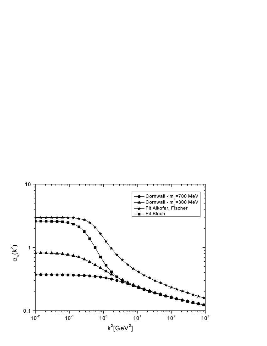
FIG. 1.: Comparison between the running couplings obtained from different solutions of Schwinger-Dyson equations.

The other expression for the running coupling constant that we will use in the next sections is the one determined by Cornwall many years ago [4]

$$\alpha_{sC}(q^{2})=\frac{4\pi}{\beta_{0}\ln\left[(q^{2}+4M_{g}^{2}(q^{2}))/\Lambda^{2}\right]},$$ (4)

where $M_{g}(q^{2})$ is a dynamical gluon mass given by,

$$M^{2}_{g}(q^{2})=m_{g}^{2}\left[\frac{\ln\left(\frac{q^{2}+4{m_{g}}^{2}}{\Lambda^{2}}\right)}{\ln\left(\frac{4{m_{g}}^{2}}{\Lambda^{2}}\right)}\right]^{-12/11}$$ (5)

$\Lambda$($\equiv\Lambda_{QCD}$) is the QCD scale parameter. This solution is the only one that has been obtained in a gauge invariant procedure. The gluon mass scale has to be found phenomenologically. A typical value is [4, 17]

$$m_{g}=500\pm 200\quad{\textnormal{M}eV}$$ (6)

for $\Lambda=300$ MeV. The Bloch and Cornwall’s expression at large momenta map perfectly into the perturbative running coupling, as can be seem in Fig.(1). We will refer to these different results as model A, B and C respectively.

III $\tau$–Lepton Decay Rate into Nonstrange Hadrons

The tests of the running coupling constant behavior that we shall discuss will depend on the exchange of gluons at different levels, i.e. the softer is the exchanged gluon the more we can test the nonpertubative behavior of $\alpha_{s}$. The physics of the $\tau$-lepton decay rate into nonstrange hadrons is one where QCD can be confronted with experiment to a very high precision. The measurement of $\alpha_{s}$ in these decays and its comparison with the nonperturbative expressions will correspond to what can be called our most perturbative test.

The normalized $\tau$-lepton decay rate into nonstrange hadrons ($h_{S=0}$) is given by [18]

$$\left.R(\tau)\right|_{S=0} = \frac{\Gamma(\tau\rightarrow h_{S=0}\nu)}{\Gamma(\tau\rightarrow l\overline{\nu}\nu)}$$ (7)

$$= N_{c}\left|V_{ud}\right|^{2}S_{ew}(1+\delta_{ew}+\delta_{P}+\delta_{NP}),$$ (8)

where $N_{c}$ is the number of colors, the flavor mixing matrix element is $\left|V_{ud}\right|^{2}=0.9511\pm 0.0014$ and $S_{ew}=1.0194$ and $\delta_{ew}=0.001$ are electroweak corrections. The nonperturbative corrections are small and consistent with zero, $\delta_{NP}=-0.003\pm 0.003$. In particular, these corrections are not directly related to the nonperturbative infrared behavior of $\alpha_{s}$. The term $\delta_{P}$ represents the perturbative QCD effects and its value can be calculated if we have $\left.R(\tau)\right|_{S=0}$. With the experimental result obtained by the ALEPH Collaboration[19], $\left.R(\tau)\right|^{expt}_{s=0}$=3.492$\pm 0.016$, and the other values above one can estimate the perturbative corrections:

$$\delta^{expt}_{P}=0.203\pm 0.007.$$ (9)

On the other hand $\delta_{P}$ can be calculated in the framework of perturbative QCD and, in the $\overline{\mbox{MS}}$ scheme, is given by the expansion

$$\delta^{th}_{P}=\left(\frac{\alpha_{s}}{\pi}\right)+5.2023\left(\frac{\alpha_{s}}{\pi}\right)^{2}+26.366\left(\frac{\alpha_{s}}{\pi}\right)^{3}+\cdots\,,$$ (10)

where $\alpha_{s}$ is the running coupling constant taken at the scale of the $\tau$-lepton mass $M_{\tau}=1.777$GeV. Substituting Eq.(9) in the left hand side of Eq.(10) and solving the resulting polynomial equation in $\alpha_{s}$ one obtain

$$\alpha^{expt}_{s}=0.3404\pm 0.0073.$$ (11)

Now we can compare the above experimental result with the different values of the nonperturbative running coupling at the $\tau$-lepton mass scale. Some comments are in order before such comparison is performed. The nonperturbative couplings have been obtained in the case of zero flavors. When we compare the perturbative to the nonperturbative results it should be understood that the introduction of fermions will affect the three models in the same direction (increasing $\alpha_{s}(0)$) and this effect would be small for a small number of flavors [4, 5]. Another point is that Eq.(10) has a renormalization scheme dependence, while the nonperturbative solutions have been obtained in one unrelated approach. However the nonperturbative couplings of the three models are obtained forcing the matching with the perturbative running coupling at very large momenta and at leading order there is no problem with scheme dependence, in such a way that the comparison can be made but not with the precision of the experimental result. Using Eqs. (1) to (4) (with $m_{g}=500$ MeV and $\Lambda=300$ MeV) instead of the perturbative running coupling we obtain

$$\alpha_{sA}=0.676\;,\quad\alpha_{sB}=0.354\;,\quad\alpha_{sC}=0.348.$$ (12)

As one could expect only the last two results are compatible with Eq.(11), and the model A fail at a level much above the one where we could claim that any scheme dependence is important. This shows the importance of the scale used to fix the coupling constant. Note that Alkofer and Fischer [9] (model A) constrain the coupling comparing its value to the experimental one of $\alpha_{s}(M_{Z})$, which seems to be the most rigorous way of doing it, unfortunately their calculation lead to a value $\Lambda_{QCD}=715$MeV, which is too high when compared to most of the values found in the literature. As the $\tau$-lepton mass scale is one where we believe that perturbative QCD can already be applied we have to conclude that the SDE solutions of model A does not describe the experimental data at such energies. Model B does it quite well but it was fitted to a smaller $\Lambda_{QCD}$ value. Note that the model A does not fit the data not because it has a large value for $\alpha_{s}(0)$, which is not so different from the model B, but because the running coupling of model A decreases much more slowly.

As we claimed previously, this test is the most perturbative one in the sense that it does not involve the introduction of hadronic wave functions directly in the calculation. In the next sections we always will need to introduce some extra hadronic information besides the coupling and gluon propagator. It is important to stress that this result does not settle the question about which one is the correct solution of gluonic SDE, it only give hints to which approximations may be or not suitable to be performed when solving these equations.

IV Effects of a frozen coupling constant in the amplitudes of the $\chi_{c2}\rightarrow\rho\rho$ decay

It is known, for a long time, that a dynamical gluon mass can affect quarkonium decays [4, 20, 21]. In the study of Refs. [20, 21] it can be noted that the dynamical mass effect is relevant in the study of their hadronic decays mostly due to phase space factors. Therefore not all quarkonium decays are good candidates to probe the infrared behavior of the running coupling constant, because the effects of phase space overwhelms the changes in the running coupling.

It is also known that the exclusive quarkonium production in $p\bar{p}$ or $pp$ interactions and subsequent decay is strongly dependent on the internal structure of the hadrons involved, which are described by their hadronic wave functions. In the inclusive case the important dependence is on the distribution function. Perturbative QCD fixes the asymptotic form of these functions as $q^{2}\rightarrow\infty$ and their general evolution, but in any realistic calculation they have to be taken as phenomenological quantities, to be experimentally determined via a set of physical information and then used in other processes.

Even when we are dealing with heavy quarks, and try to propose tests for the interface between perturbative and non-perturbative QCD, we verify that we cannot test the infrared behavior of quarks and gluons vertex and propagators independently of hadronic wave or distribution functions. In this Section we discuss the effects of a frozen coupling constant in the measurement of the $\rho$ vector meson helicity density matrix that are produced in the $\chi_{c2}\rightarrow\rho\rho$ decay. This is a case where the infrared behavior of the coupling is entangled with the behavior of the wave or distribution functions. We advance that in Section V we will discuss a more ordinary case where the wave function is well known, and where it is possible to study the QCD infrared behavior with less uncertainty [17].

Some time ago Anselmino and Murgia [22] considered the $\chi_{c2}\rightarrow\rho\rho$ decay process of polarized charmonium states created in $p\bar{p}$ or $pp$ interactions and have shown how the observation of the polarization of the vector meson, via a measurement of its diagonal helicity density matrix elements, neatly depends on the $\rho$ wave function and helps in discriminating between different kinds of these quantities.

The study of Ref.[22] provide an interesting arena to introduce the effects of a frozen running coupling constant. Our result will show that depending on the form of the wave function we could observe a larger or smaller effect of the freezing in the infrared, showing how the nonperturbative behaviors of wave (or distribution) functions with the ones of the effective coupling can become entangled.

The processes that we consider are the exclusive

$$p\overline{p}\rightarrow\chi_{c2}\rightarrow\rho\rho$$ (13)

or the inclusive

$$pp\rightarrow\chi_{c2}+X\rightarrow\rho\rho+X$$ (14)

production of a pair of $\rho$ vectors with the subsequent decay

$$\rho\rightarrow\pi\pi,$$ (15)

and the quantity experimentally observed is the angular distribution of either one of the pions in the helicity rest frame of the decaying $\rho$.

The pion angular distribution depends of the spin state of the $\rho$ via the elements of its helicity density matrix $\rho_{\lambda,\lambda^{\prime}}(\rho)$:

$$W(\Theta,\Phi) = \frac{3}{4\pi}[\rho_{0,0}\cos^{2}{\Theta}+(\rho_{1,1}-\rho_{1,-1})\sin^{2}{\Theta}\cos^{2}{\Phi}+(\rho_{1,1}+\rho_{1,-1})\sin^{2}{\Theta}\sin^{2}{\Phi}$$ (17)

$$-\sqrt{2}(Re\rho_{1,0})\sin 2{\Theta}\cos{\Phi}],$$

where $\Theta$ and $\Phi$ are, respectively, the polar and azimuthal angles of the pion as it emerges from the decay of the $\rho$, in the $\rho$ helicity rest frame. Eq. (17) can be integrated over $\Theta$ or $\Phi$ generating polar and azimuthal distributions, which can be measured and give information on $\rho_{\lambda,\lambda^{\prime}}(\rho)$. The details of this procedure (i.e. the vector meson helicity density matrix calculation for massless quarks) can be found in Ref.[22] and references therein.

The helicity density matrix of the $\rho$ meson are [22]

$$\rho_{\lambda,\lambda^{\prime}}=0,\,\,\,\,\,\lambda\neq\lambda^{\prime},\,\,\,\,\,\,\,\,\,\,\,\,\,\,\,\,\,\,\,\rho_{0,0}=1-2\rho_{1,1}$$ (18)

$$\rho_{1,1}=\rho_{-1,-1}=\frac{1}{2}\frac{1}{1+3\frac{|\mbox{\~{A}}_{0,0}|^{2}}{|\mbox{\~{A}}_{1,-1}|^{2}}F(\theta)},$$ (19)

where the reduced amplitudes ${\tilde{A}}_{\lambda,\lambda^{\prime}}$ are given in Eqs. (2.10), (2.11) and (2.14), (2.15) of Ref.[23] and do not depend on the $\rho$ production angles $\theta$ and $\phi$, but do depend on the wave functions. Eq. (19) has the same form both for exclusive and inclusive $\rho$ production, but the dependence on the production angle $\theta$ is different in the two cases

$$F^{ex}(\theta)=\frac{\cos^{2}(\theta)}{1+\cos^{2}(\theta)},$$ (20)

$$F^{in}(\theta)=\frac{\sin^{4}(\theta)}{1+6\cos^{2}(\theta)+\cos^{4}(\theta)}.$$ (21)

The ratio of reduced amplitudes $|\mbox{\~{A}}_{0,0}|^{2}/|\mbox{\~{A}}_{1,-1}|^{2}$ appearing in Eq.(19) are computed as a function of the $\rho$ longitudinally $(L,\lambda=0)$ and transversely $(T,\lambda=\pm 1)$ polarized vector mesons wave functions, which are indicated respectively by $\varphi_{L}$ and $\varphi_{T}$, and correspondent decay constants given by $f_{L}$ and $f_{T}$. This ratio is equal to [22]

$$\frac{|\mbox{\~{A}}_{0,0}|}{|\mbox{\~{A}}_{1,-1}|}=\frac{1}{\sqrt{6}}\left(\frac{f_{L}}{f_{T}}\right)^{2}\frac{|I_{0,0}|}{|I_{1,-1}|}$$ (22)

where

$$I_{1,-1}=-\frac{1}{32}\int^{1}_{0}\,dxdy\varphi_{T}(x,\mbox{\~{Q}}_{x}^{2})\varphi_{T}(y,\mbox{\~{Q}}_{y}^{2})\frac{\alpha_{s}(xyM^{2}_{\chi})\alpha[(1-x)(1-y)M^{2}_{\chi}]}{xy(1-x)(1-y)(2xy-x-y)}$$ (23)

$$I_{0,0}= - \frac{1}{32}\int^{1}_{0}\,dxdy\varphi_{L}(x,\mbox{\~{Q}}_{x}^{2})\varphi_{L}(y,\mbox{\~{Q}}_{y}^{2})\frac{\alpha_{s}(xyM^{2}_{\chi})\alpha[(1-x)(1-y)M^{2}_{\chi}]}{xy(1-x)(1-y)(2xy-x-y)}\left[1+\frac{(x-y)^{2}}{2xy-x-y}\right].$$ (24)

In the above equations $M_{\chi}=3.6\,\mbox{GeV}$ is the $\chi_{c2}$ mass and $\mbox{\~{Q}}_{x}=\min(x,1-x)Q$.

To calculate the helicity density matrix $\rho_{1,1}$ we choose two different sets of $\varphi_{L}$ and $\varphi_{T}$: a set of symmetric distribution amplitudes

$$\varphi_{L}=\varphi_{T}=6x(1-x)$$ (25)

and the QCD sum rules amplitudes [24]

$$\varphi_{L}(x, \mbox{\~{Q}}_{x}^{2} )=6x(1-x)\left\{1+\frac{1}{5}C_{2}^{3/2}(2x-1)\left[\frac{\alpha_{s}(\mbox{\~{Q}}^{2}_{x})}{\alpha_{s}(\mu_{L}^{2})}\right]^{2/3}\right\}$$ (26)

$$\varphi_{T}(x,\mbox{\~{Q}}_{x}^{2})=6x(1-x)\left\{\left[\frac{\alpha_{s}(\mbox{\~{Q}}^{2}_{x})}{\alpha_{s}(\mu_{T}^{2})}\right]^{4/25}\right.\left.-\frac{1}{6}C_{2}^{3/2}(2x-1)\left[\frac{\alpha_{s}(\mbox{\~{Q}}^{2}_{x})}{\alpha_{s}(\mu_{T}^{2})}\right]^{52/75}\right\}$$ (27)

where $\mu_{L}^{2}=0.5\,(\mbox{GeV}/c)^{2}$, $\mu_{T}^{2}=0.25\,(\mbox{GeV}/c)^{2}$, and $C_{z}$ denotes Gegembauer polynomials. In both cases we assume $f_{L}=f_{T}$.

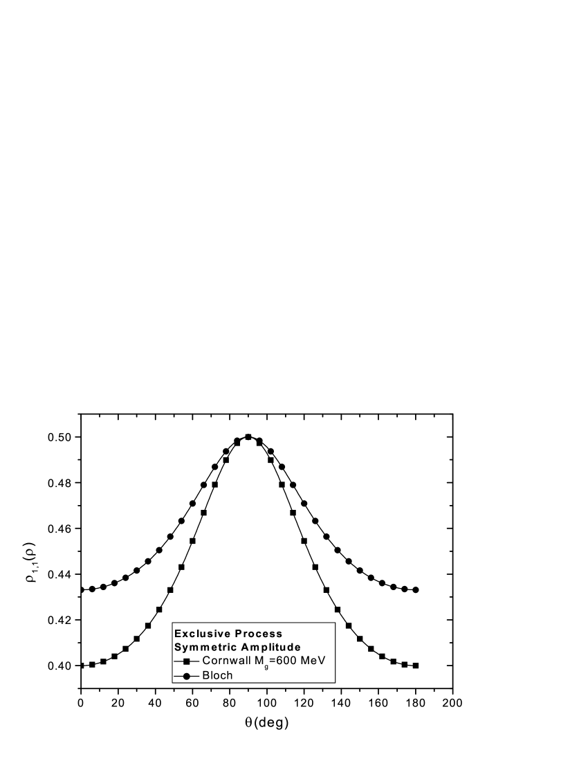
FIG. 2.: Values of the helicity matrix element $\rho_{1,1}$ as a function of the $\rho$-meson production angle $\theta$. The exclusive process is computed with the symmetric distribution amplitudes for the Bloch and Cornwall’s coupling constants.

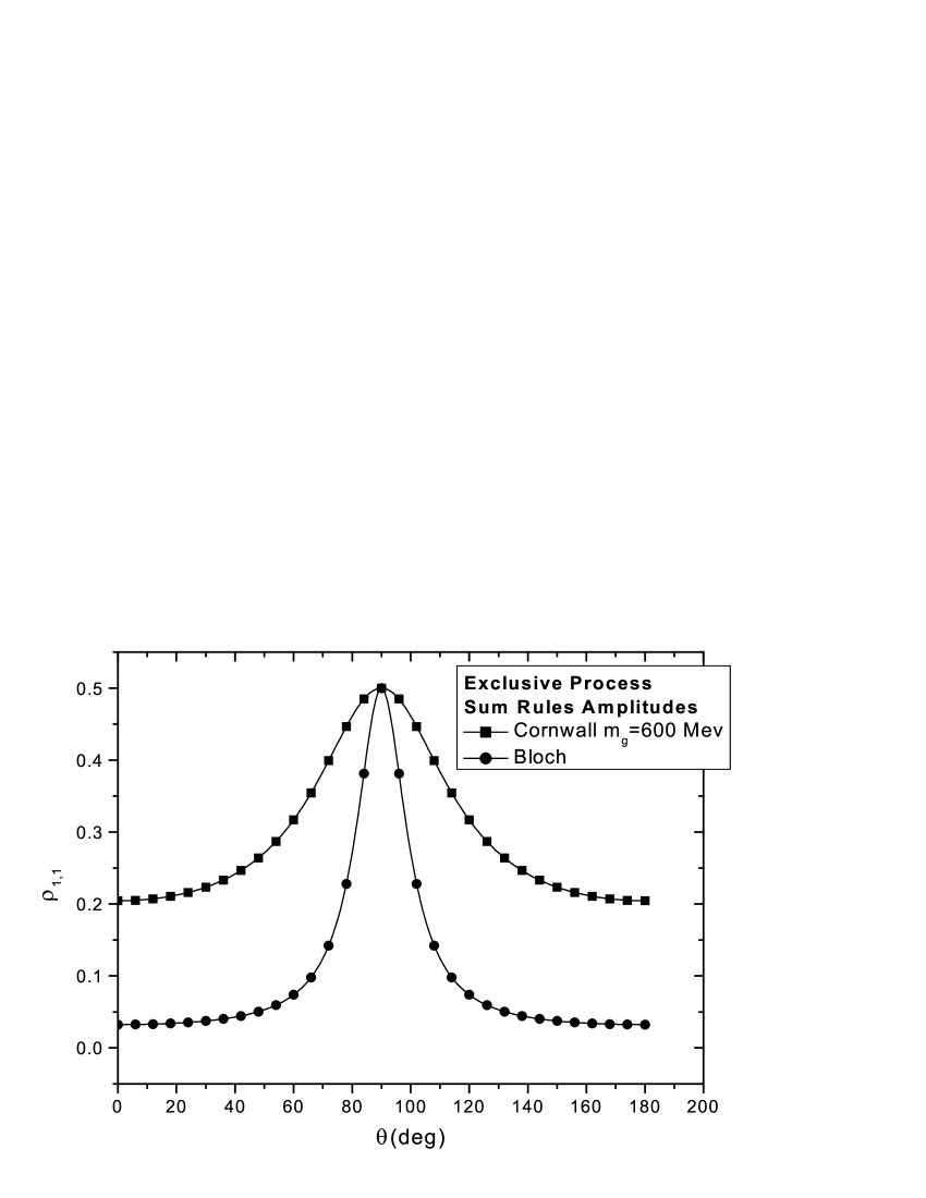
FIG. 3.: Same notation as in Fig.(2) but calculated with QCD sum rules distribution amplitudes

Our results for the exclusive process (Eq.(13)) are displayed in Fig.(2) and Fig.(3). Fig.(2) shows $\rho_{1,1}$ as a function of the $\rho$-meson production angle $\theta$, computed with the symmetric wave function whereas Fig.(3) was calculated with the QCD sum rule amplitudes. Both figures show curves for different behaviors of the running coupling constant, the one of Eq.(3) obtained by Bloch and the one of Eq.(4) obtained by Cornwall with $m_{g}=600$ MeV and $\Lambda=300$ MeV. The calculations for model A are not shown in the figures. The results for this model are similar to the ones of model B with curves located in the opposite direction to the curves of model C.

FIG. 4.: Values of the helicity matrix element $\rho_{1,1}$ as a function of the $\rho$-meson production angle $\theta$ in the case of inclusive $\chi_{c2}$ production. The curves were obtained using the symmetric distribution amplitudes and the expressions of Eq.(3) and Eq.(4) for the coupling constant.

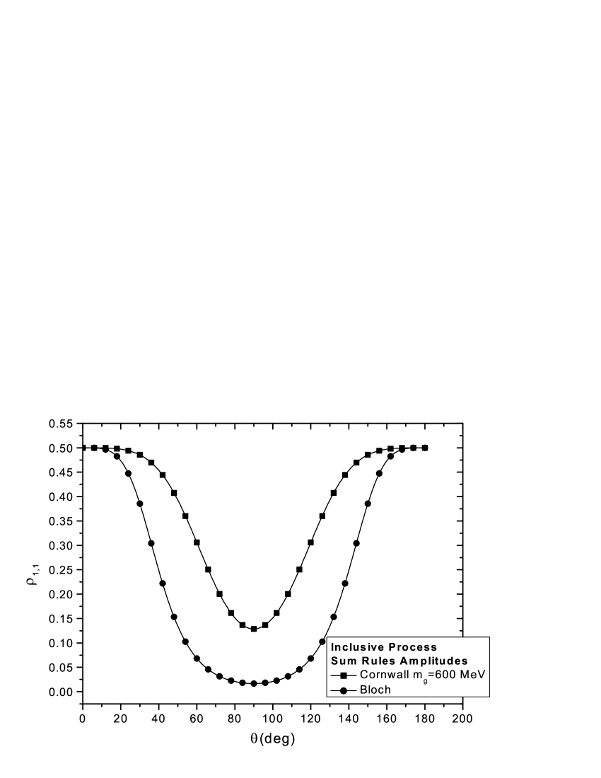
FIG. 5.: Same notation as in Fig.(4) but calculated with QCD sum rules distribution amplitudes

As claimed by Anselmino and Murgia [22] the measurement of the helicity matrix element $\rho_{1,1}$ of the vector meson in the $\chi_{c2}\rightarrow\rho\rho$ can indeed discriminate differences between wave (or distribution) functions, but the effect of different running couplings is not negligible and one effect can mask the other. Of course, this is not an easy experiment, but is a feasible one. If the measurement is performed with high precision it can provide information about the infrared behavior of the coupling constant.

The curves for the inclusive process (Eq.(14)) are displayed in Fig.(4) and Fig.(5). Fig.(4) shows $\rho_{1,1}$ as a function of the $\rho$-meson production angle $\theta$, computed with the symmetric distribution amplitude whereas Fig.(5) was calculated with the QCD sum rule amplitudes. The differences in the curves are of the same order as in the exclusive case.

Note that in both cases (exclusive or inclusive) the values of $\rho_{1,1}$ is modified by a factor of $O(2-3)$ when we use the wave functions obtained through QCD sum rules. This is expected because they have a stronger dependence on $\alpha_{s}(q^{2})$. The difference occurs at different angles for the exclusive and inclusive $\chi_{c2}$ production. Actually, it is surprising that in such a delicate experiment, where the effects of the running coupling appear in a ratio like the one described by Eq.(22), there is still a clear signal of the dependence on the infrared value of the coupling constant. In this section we verified how the infrared behavior of the coupling can be masked by the nonperturbative wave functions. In the next sections we will look at processes where the effects of wave or distribution functions are not so pronounced or are better known.

V The $\gamma\rightarrow\pi_{0}$ transition form factor

When making predictions within perturbative QCD, we are always confronted with problems like the choice of distribution amplitudes as discussed in the previous section, the choice of renormalization scale $\mu$ and scheme for the coupling constant, etc… However there are calculations that have been discussed extensively in the literature, processes where the measurement is more sensitive only to the asymptotic distribution amplitude of a particular hadron, and where an optimal renormalization scale has been estimated. This was the case of the pion form factor discussed in Ref.[5], and is the case of the $\gamma\rightarrow\pi_{0}$ transition form factor to be described here.

The photon-to-pion transition form factor $F_{\gamma\pi}(Q^{2})$ is measured in single-tagged two-photon $e^{+}e^{-}\rightarrow e^{+}e^{-}\pi^{0}$ reactions. The amplitude for this process has the factorized form

$$F_{\gamma\pi}(Q^{2})=\frac{4}{\sqrt{3}}\int^{1}_{0}\,dx\,\phi_{\pi}(x,Q^{2})T^{H}_{\gamma\pi}(x,Q^{2}),$$ (28)

where the hard scattering amplitude $T^{H}_{\gamma\pi}(x,Q^{2})$ is given by

$$T^{H}_{\gamma\pi}(Q^{2})=\frac{1}{(1-x)Q^{2}}[1+{\cal O}(\alpha_{s})].$$ (29)

Using an asymptotic form for the pion distribution amplitude $\phi_{\pi}=\sqrt{3}f_{\pi}x(1-x)$ we obtain [25]

$$Q^{2}F_{\gamma\pi}(Q^{2})=2f_{\pi}\left(1-\frac{5}{3}\frac{\alpha_{V}(Q^{\ast})}{\pi}\right)$$ (30)

where $Q^{\ast}=\exp^{-3/2}Q$ is the estimated Brodsky-Lepage-Mackenzie scale for the pion form factor in the scheme discussed in Ref.[25].

In Fig.(6) we compare the photon to pion transition form factor with CLEO data [26]. The curves were computed with different expressions for the infrared behavior of the running coupling constant. We assumed $f_{\pi}\simeq 93\;\mbox{MeV}$ and $\Lambda=300$ MeV. Using the running coupling constant given by the expression of Eq.(3) we obtain a fit for the photon-pion transition form factor very far from the experimental data. The result obtained when we use Eq.(1) is not shown and gives an even worse fit. The infrared value of the coupling constant is so large in the case of the coupling constants given by Eqs.(3) and (1), that we are not sure that the perturbative result can be trusted even at such large momentum scale.

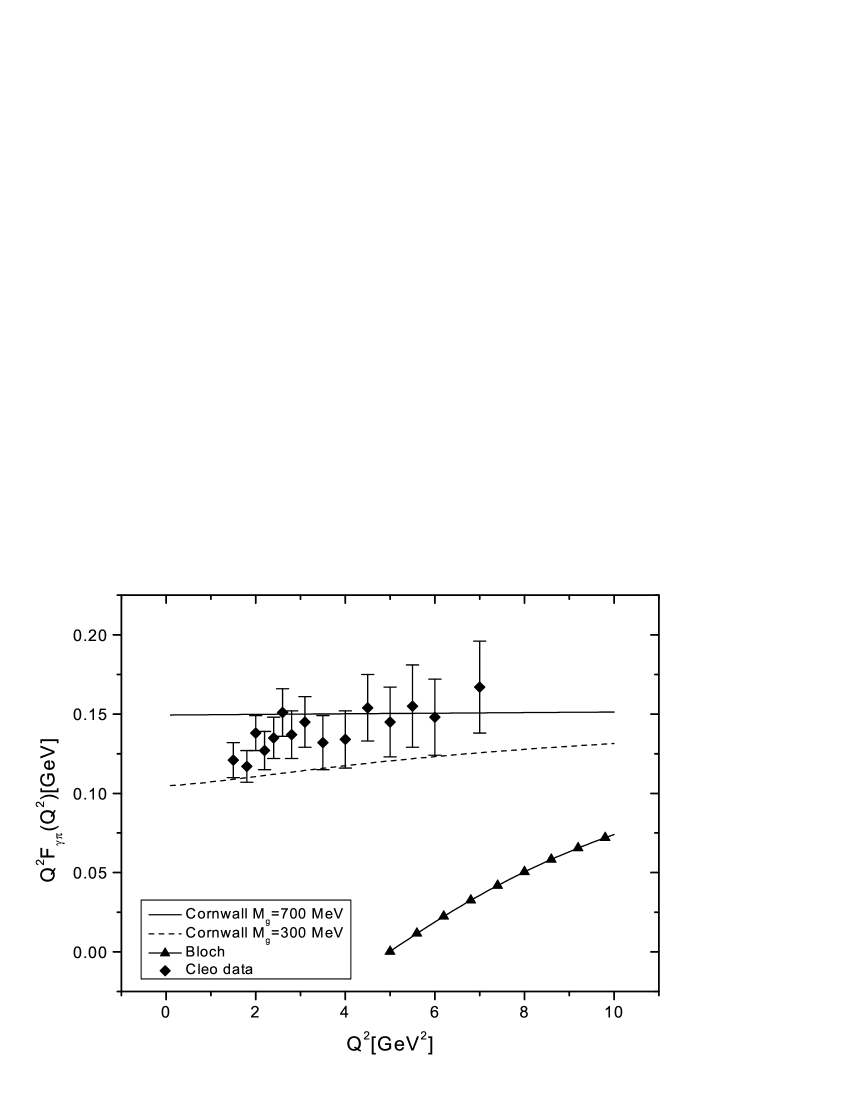
FIG. 6.: The $\gamma\rightarrow\pi^{0}$ transition form factor calculated with different expressions for the infrared behavior of the running coupling constant.

The infrared coupling constants related to the class of SDE solutions consistent with an infrared finite propagator that vanishes at origin of momenta, are much stronger than most of the phenomenological estimates of the frozen $\alpha_{s}(0)$ value that we quoted in Ref.[5] ($\alpha_{s}(0)\approx 0.7\pm 0.3$), and are at the origin of the strange lower curve of Fig.(6). Notice that due to the large scale of momenta involved in this process it is not expected that higher order corrections are still important. The data is only compatible with Eq.(4), which has a smoother increase towards the infrared region. Perhaps this behavior is actually indicating that the transition to the infrared should be a soft one. Again the result for model A is not shown because it is even worse than the one of model B.

Note that in Fig.(6) the curves obtained with the Cornwall’s coupling constant do not show large variation in the full range of uncertainty of the dynamical gluon mass (see Eq.(6)). It is interesting that its behavior is quite stable in this case as well as for the pion form factor studied in Ref.[5]. If we had large variations of the infrared coupling constant with the gluon mass scale we could hardly propose any reliable phenomenological test for its freezing value. We stress that the results are obtained for a perturbative scale of momenta and it seems that we have to choose between two possibilities: This process cannot be predicted by perturbative QCD up to a scale of several GeV, or some of the ESD solutions are predicting a too large value of the coupling constant in the infrared and the approximations made to determine these solutions are too crude.

VI Elastic differential cross section for pp scattering

We have verified in Section IV one case where the behavior of the coupling constant in the infrared is entangled with the one of the distribution amplitudes. In Section V it was shown a classic QCD calculation where the asymptotic behavior of the wave function is more important than the infrared one, leading to a cleaner test for the nonperturbative behavior of the coupling constant. Here we will discuss a test for the infrared QCD behavior that makes use of a phenomenological model for diffractive interactions [17]. In this case we will also make use of a hadronic wave function, but the main source of uncertainty is in the fact that we assume a model for elastic scattering containing a series of approximations, which are beyond the scope of a pure QCD calculation.

We will compute the elastic differential cross section for pp scattering within the Landshoff-Nachtmann model (LN) for the Pomeron exchange [27]. As discussed in Refs.[17, 28], this is a model where the Pomeron is represented by two-gluons exchange, and it is particularly dependent on the infrared properties of the gluon, not only on the coupling constant but also on the behavior of the gluon propagator. In this model one of the gluons carry most of the momentum exchanged in the interaction while the other seems to appear just to form the colorless Pomeron. Therefore besides the coupling constant we will also need the expressions for the gluon propagators obtained through the solutions of the SDE, although this dependence with the nonperturbative behavior of the gluon propagator is important only when the gluon is exchanged at low momentum. The gluon propagator in Landau gauge is written as

$$D_{\mu\nu}(q^{2})=\left({\delta}_{\mu\nu}-\frac{q_{\mu}q_{\nu}}{q^{2}}\right)D(q^{2}),$$ (31)

where the expression for $D(q^{2})$ obtained by Cornwall is given by

$$D^{-1}(q^{2})=\left[q^{2}+M_{g}^{2}(q^{2})\right]bg^{2}\ln\left[\frac{q^{2}+4M^{2}_{g}}{\Lambda^{2}}\right].$$ (32)

We will also make use of the running coupling constant obtained by Fischer and Alkofer (model A) and their respective propagator $D(q^{2})=Z(q^{2})/q^{2}$, where $Z(q^{2})$, in Landau gauge, is fitted by

$$Z(x)=\left(\frac{\alpha_{sA}(x)}{\alpha_{A}(\mu)}\right)^{1+2\delta}R^{2}(x),$$ (33)

and

$$R(x)=\frac{cx^{\kappa}+dx^{2\kappa}}{1+cx^{\kappa}+dx^{2\kappa}}$$ (34)

where the constants appearing in Eq.(33) and Eq.(34) are given by

$\alpha_{A}(\mu^{2})=0.9676$,

$\kappa=0.5953$,

$\delta=-9/44$,

$c=1.8934\;\mbox{GeV}^{-2\kappa}$,

$d=4.6944\;\mbox{GeV}^{-4\kappa}$.

In the LN model the elastic differential cross can be obtained from

$$\frac{d\sigma}{dt}=\frac{|A(s,t)|^{2}}{16\pi s^{2}}$$ (35)

where the amplitude for elastic proton-proton scattering via two-gluon exchange can be written as

$$A(s,t)=is8\alpha_{s}^{2}\left[T_{1}-T_{2}\right]$$ (36)

with

$$T_{1}=\int\,d^{2}kD\left(\frac{q}{2}+k\right)D\left(\frac{q}{2}-k\right)|G_{p}(q,0)|^{2}$$ (37)

$$T_{2}=\int\, d^{2}kD\left(\frac{q}{2}+k\right)D\left(\frac{q}{2}-k\right)G_{p}\left(q,k-\frac{q}{2}\right)\left[2G_{p}(q,0)-G_{p}\left(q,k-\frac{q}{2}\right)\right]$$ (38)

where $G_{p}(q,k)$ is a convolution of proton wave functions

$$G_{p}(q,k)=\int\,d^{2}pd\kappa\psi^{\ast}(\kappa,p)\psi(\kappa,p-k-\kappa q).$$ (39)

$G_{p}(q,0)$ is given by the Dirac form factor of the proton

$$F_{1}(t)=G_{p}(q,0)=\frac{4m^{2}-2.79t}{4m^{2}-t}\frac{1}{(1-t/0.71)^{2}}.$$ (40)

To estimate $G_{p}(q,k-q/2)$ we assume a proton wave function peaked at $\kappa=1/3$ and obtain

$$G_{p}\left(q,k-\frac{q}{2}\right)=F_{1}\left(q^{2}+9\left|k^{2}-\frac{q^{2}}{4}\right|\right)$$ (41)

Eq.(35) to Eq.(41) can be computed using the couplings and propagators discussed above. We compare the differential elastic cross-section for proton-proton scattering with the experimental data of Breakstone et al. at $\sqrt{s}=53\quad{\textnormal{G}eV}$ [29]. The results have to be adjusted by a normalization factor $s^{0.168}$ which accounts for the energy dependent part of ${d\sigma}/{dt}$ [30]. For large $|t|$ values, double-Pomeron exchange and three-gluon exchange are known to be important; we therefore do not expect to describe the data near and above $-t\simeq 0.5\quad{\textnormal{G}eV}^{2}$ [30, 31]

The data of elastic proton-proton scattering is well fitted assuming a dynamical gluon mass of $m_{g}=370\quad{\textnormal{M}eV}$ for $\Lambda=300\quad{\textnormal{M}eV}$. The calculation has a small variation with the value of $m_{g}$ and is more sensitive to the ratio $m_{g}/\Lambda$. Using the coupling and propagator of Alkofer et al. (model A) we obtain a curve that is about one order of magnitude away from the experimental points. Unfortunately we do not have the propagator solution for model B and for this reason we do not show the results in this case, although we can guess that it would produce a curve in Fig.(7) between the curves of model A and C.

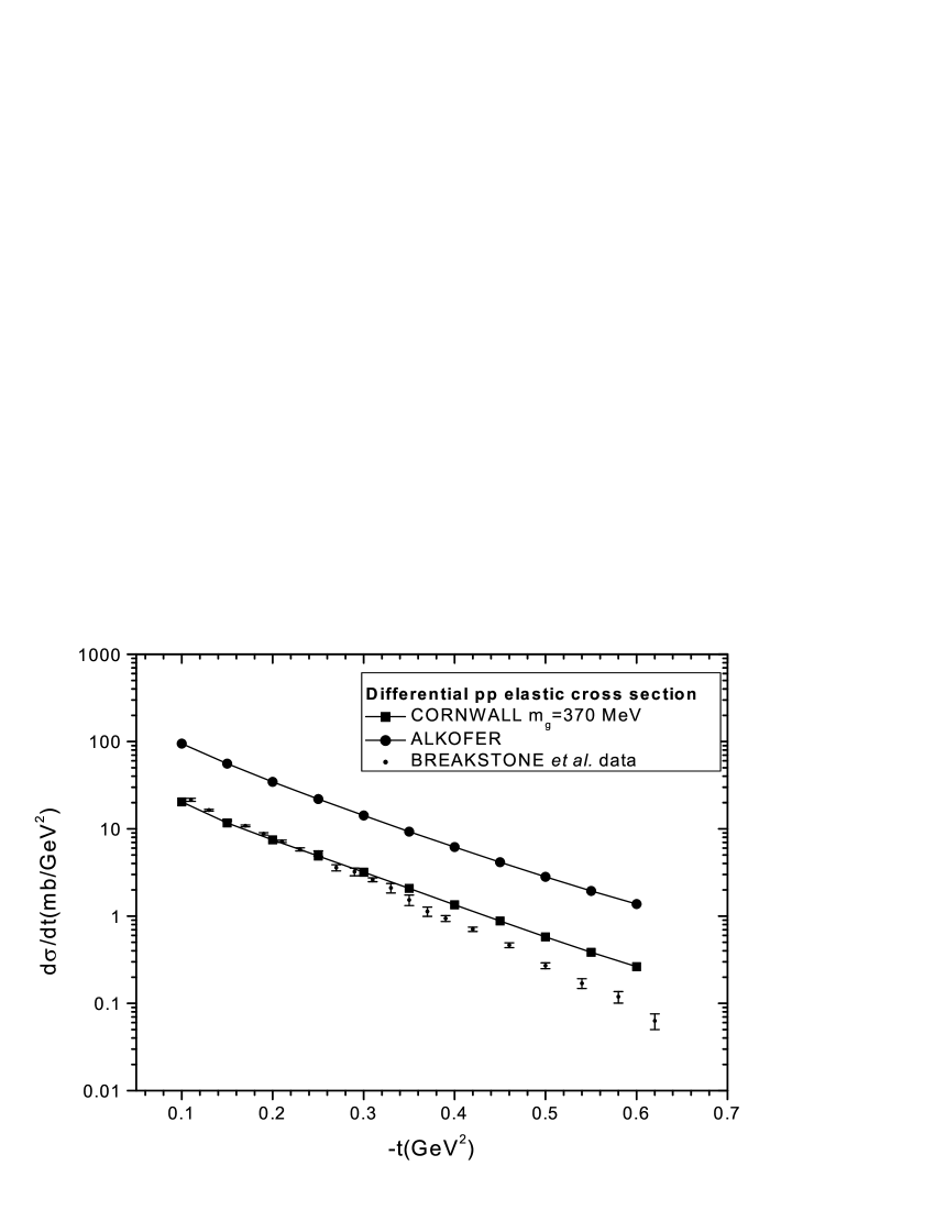
FIG. 7.: Differential $pp$ elastic cross section at $\sqrt{(}s)=53\,\mbox{GeV}$ computed within the Landshoff–Nachtmann model for the Pomeron, using different infrared couplings and gluon propagators obtained from SDE solutions.

There is a striking difference between the two classes of SDE solutions that we discussed in the Introduction. In the case of Cornwall’s solution it is the product $g^{2}D(q^{2})$ that behaves roughly as $1/{m_{g}}^{2}$ as $q^{2}\rightarrow 0$ and this product has no $g^{2}$ dependence [4]. This does not happen for the class of gluon propagators that seems to vanish at origin. As in this case the coupling is not canceled in the ${d\sigma}/{dt}$ calculation and as it is a factor of $O(3)$ larger, it is not difficult to understand the one order of magnitude difference in the result of the cross sections. This specific calculation is model dependent, however it is quite sensitive on the infrared behavior of the theory.

VII Exclusive $\rho$ Production in Deep Inelastic Scattering

Donnachie and Landshoff [32] successfully described the process $\gamma^{*}(q)\>p(P)\>\rightarrow\>\rho(r)\>p(P^{\prime})$ with a soft Pomeron exchange, and later they [33] considered Pomeron exchange as being the exchange of two gluons as in the previous section. Pursuing that idea Cudell [34] proposed the following expression for the polarized differential cross section for exclusive $\rho$ production:

$$\frac{d\sigma_{j}}{dt}=\left(\frac{\alpha_{elm}}{4w^{4}}\left|A_{j}\right|^{2}\Phi^{2}\right)\>Z^{2}\>\left[3\>F_{1}(t)\right]^{2}\>,\quad j=T,\>L,$$ (42)

where $\alpha_{elm}\simeq 1/137$ is the electromagnetic coupling constant and $w^{2}=(q+P)^{2}$. The factor $\Phi$ is given by

$$\Phi=\sqrt{\frac{f_{\rho}\>m_{\rho}}{24}},$$ (43)

where $f_{\rho}\simeq 30$MeV is the $\rho$ form factor and $m_{\rho}\simeq 770$ MeV is the $\rho$ mass.

$$Z=\left(\frac{w^{2}}{w_{0}^{2}}\right)^{0.08+\alpha^{\prime}t}\>,$$ (44)

with $w^{2}_{0}=1/\alpha^{\prime}\simeq 4$GeV². The Dirac form factor of the proton is

$$F_{1}(t)=\frac{4m^{2}_{p}-2.79t}{4m^{2}_{p}-t}\frac{1}{(1-t/0.71)^{2}},$$ (45)

where $m_{p}$ is the proton mass.

The amplitude is

$$A_{j}=i\frac{8\sqrt{2}}{3\pi}\>m_{\rho}\>P_{j}\>\int^{0}_{-\infty}\frac{dk^{2}\;(t-4k^{2})}{(\mu^{2}_{Q}-t)(\mu^{2}_{Q}-4k^{2})}\left[4\pi\alpha_{n}D\left(k^{2}+\frac{t}{4}\right)\right]^{2},$$ (46)

$$\quad\quad\mu^{2}_{Q}=m^{2}_{\rho}+Q^{2}\;,\quad j=T,\>L$$ (47)

where $P_{T}=w^{2}/2$; $P_{L}=P_{T}\cdot(m^{2}_{\rho}+Q^{2}+t)/(2m_{\rho}Q)$. In the last term of the integrand we have the frozen coupling constant $\alpha_{n}=\alpha_{s}(0)$ and the gluon propagator $D(p^{2})$.

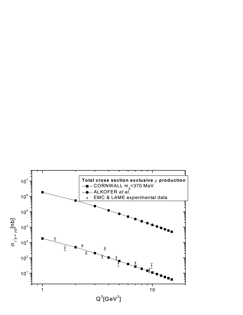
FIG. 8.: Total cross section for exclusive $\rho$ production in deep inelastic scattering.

The total cross section can be obtained through the integral

$$\sigma_{total}(Q^{2})=\int dt\>\left(\frac{d\sigma_{T}}{dt}+\varepsilon\frac{d\sigma_{L}}{dt}\right)\>,\quad\varepsilon\approx 0.85.$$ (48)

This cross section is dependent not only on the nonperturbative coupling constant but also on the gluon propagator as the calculation of the previous section. We compared the solutions of Alkofer et al. (model A) and Cornwall (model C). The reason for not using model B is the same as the one discussed in the previous section. With the running coupling constants (eqs. (1) and (4)) and their respective propagators (eqs. (33) and (32)) we obtain the results shown in Fig.(8), where they are compared with the experimental data from EMC[35] and LAME[36]. As explained in Ref.[34] the model for exclusive $\rho$ production is consistent with experiment only in the range of momenta shown in the figure, at larger values of $Q^{2}$ there are other contributions to the cross section.

VIII Conclusions

In this work we proposed phenomenological tests for the infrared behavior of running coupling constant that have been obtained through the nonperturbative solutions of Schwinger-Dyson equations of the QCD gluonic sector. We are only considering SDE solutions that are infrared finite. Although infrared divergent solutions have not been fully discarded, there are several indications that these QCD Green functions are well behaved in the infrared. Unfortunately due to the complexity of the SDE, approximations are still necessary to obtain these solutions and they lead to different expressions. Phenomenological tests are important because they are able to indicate which are the correct approximations that can be performed to solve SDE, selecting the solution that is compatible with the experimental data.

We studied the effects of a frozen coupling constant in the $\tau$-lepton decay rate into nonstrange hadrons. This is a typically perturbative test and, in particular, it shows the importance of the method used to fix the scale of the running coupling constant, which is different for the couplings shown in Eqs.(1) and (3) (model A and B). The measurement of the $\rho$ vector meson helicity density matrix that are produced in the $\chi_{c2}\rightarrow\rho\rho$ decay is one interesting experiment to be performed. The measurement of the diagonal matrix element provide information on the infrared behavior of the coupling constant as well as on the distribution amplitude. In this case both behaviors are entangled and a good knowledge on the distribution amplitude is needed in order to select a preferred behavior for the coupling constant. The experiment is not an easy one, but can be performed and will give information complementary to the others that we have discussed.

The effects of the infrared behavior of the coupling constant in the photon-to-pion transition form factor $F_{\gamma\pi}(Q^{2})$ is much more interesting. The calculation probes the asymptotic behavior of the pion distribution amplitude and provide a cleaner test for the freezing of the coupling constant. The differences between the existent solutions obtained from SDE for $\alpha_{s}(q^{2})$ are shown clearly in the comparison with the experimental data, which seems to select the coupling constant compatible with dynamical generation of a gluon mass.

The analysis of the differential cross section for proton-proton scattering and the cross section for exclusive $\rho$ production in deep inelastic scattering are also unambiguously selecting one specific behavior for the QCD Green functions in the infrared. In this case we made use of a model of diffractive scattering proposed by Landshoff and Nachtmann and it could be argued that the model has not been obtained from straightforward QCD calculations. However the model has a great success in the explanation of diffractive physics at low energy, and again the comparison with experimental data is consistent with the result obtained from the other phenomenological tests. Diffraction in this model is explained through the exchange of two gluons, where one of the gluons carries most of the momentum and the other is soft. Therefore the model actually probes the infrared region.

It is worth mentioning the influence of gauge invariance and presence of fermions in the solutions for the coupling constants that we have discussed. The Cornwall’s solution was obtained in a gauge invariant procedure, the others were obtained in Landau gauge. We do not expect that gauge invariance introduce a large effect in the result. In general solutions of SDE are relatively stable in respect to changes in the gauge choice, and we should expect that if the solutions minimize the vacuum energy the gauge dependence should disappear. The effect of the number of flavors in Cornwall’s solution[4] is not so strong, and it appears in the coefficient $\beta_{0}$ of the coupling constant and in the gluon mass equation increasing the value of the frozen coupling. If a nonzero number of flavors produces any observable effect, this one should act in the same sense for all solutions. Therefore, we do not expect large changes in our results with the inclusion of fermion loops in the SDE solutions.

We conclude pointing out that Schwinger-Dyson equations provide a powerful tool to investigate the QCD infrared behavior. These are complicated equations whose solutions are determined only after some specific approximations leading to different expressions. These expressions can be phenomenologically tested, indicating which are the most reliable approximations. In the tests presented here only one solution, consistent with a dynamically generated mass for the gluon, was shown to be compatible with the experimental data.

REFERENCES

- [1] Yu. L. Dokshitzer and B. R. Webber, Phys. Lett. B352 (1995) 451; Yu. L. Dokshitzer, G. Marchesini and B. R. Webber, Nucl. Phys. B469 (1996) 93; Yu. L. Dokshitzer, Plenary talk at ICHEP 98, Proc. Vancouver 1998, High energy physics, Vol. 1, 305-324, hep-ph/9812252; P. Hoyer, Proc. 6th INT-Jlab Workshop, Newport News, VA, May 1999, hep-ph/9303262.
- [2] A. C. Mattingly and P. M. Stevenson, Phys. Rev. Lett. 69 (1992) 1320; Phys. Rev. D49 (1994) 437.
- [3] S. J. Brodsky, hep-ph/0111127; Acta Phys. Polon. B32 (2001) 4013, hep-ph/0111340; Fortsch. Phys. 50 (2002) 503.
- [4] J. M. Cornwall, Phys. Rev. D26 (1982) 1453.
- [5] A. C. Aguilar, A. Mihara and A. A. Natale, Phys. Rev. D65 (2002) 054011.
- [6] H. Gies, Phys.Rev. D66 (2002) 025006.
- [7] K. Langfeld, H. Reinhardt and J. Gattnar, Nucl. Phys. B621 (2002) 131; hep-lat/0110025; L. Giusti, M. L. Paciello, S. Petrarca, B. Taglienti and N. Tantalo, hep-lat/0110040; A. Cucchieri and D. Zwanziger, hep-lat/0012024; C. Alexandrou, Ph. de Forcrand and E. Follana, hep-lat/0112043; hep-lat/0203006.
- [8] J. C. R. Bloch, Phys. Rev. D66 (2002) 034032.
- [9] C. S. Fischer, R. Alkofer and H. Reinhardt, Phys. Rev. D65 (2002) 094008; C. S. Fischer and R. Alkofer, Phys. Lett. B536 (2002) 177; R. Alkofer, C. S. Fischer and L. von Smekal, Acta Phys. Slov. 52 (2002) 191, hep-ph/0205125.
- [10] C. Lerche and L. von Smekal, Phys. Rev. D65 (2002) 125006.
- [11] D. Zwanziger, Phys. Rev. D65 (2002) 094039.
- [12] R. Alkofer and L. von Smekal, Phys. Rept. (2001, in press), hep-ph/0007355; L. von Smekal, A. Hauck and R. Alkofer, Ann. Phys. 267 (1998) 1; L. von Smekal, A. Hauck and R. Alkofer, Phys. Rev. Lett. 79 (1997) 3591.
- [13] S. J. Brodsky, E. Gardi, G. Grunberg and J. Rathsman, Phys. Rev. D63 (2001) 094017 and references therein.
- [14] A. A. Natale and P. S. Rodrigues da Silva, Phys. Lett. B392 (1996) 444 ; J. C. Montero, A. A. Natale and P. S. Rodrigues da Silva, Prog. Theor. Phys. 96 (1996) 1209.
- [15] A. M. Badalian and Yu. A. Simonov, Phys. At. Nucl. 60 (1997) 630; A. M. Badalian and V. L. Morgunov, Phys. Rev. D60 (1999) 116008; A. M. Badalian and B. L. G. Bakker, Phys. Rev. D62 (2000) 094031.
- [16] D. V. Shirkov and I. L. Solovtsov, Phys. Rev. Lett. 79 (1997) 1209; see also D. V. Shirkov, hep-th/0210013 and references therein.
- [17] F. Halzen, G. Krein, and A. A. Natale, Phys. Rev. D47 (1993) 295.
- [18] J. G. Koerner, F. Krajewski and A. A. Pivovarov, Phys. Rev. D63 (2000) 036001 and references there in.
- [19] ALEPH Collaboration, Z. Phys. C76 (1997) 15; Eur. Phys. J. C4 (1998) 409.
- [20] G. Parisi and R. Petronzio, Phys. Lett. B94 (1980) 51 .
- [21] A. Mihara and A. A. Natale, Phys. Lett. B482 (2000) 378.
- [22] M. Anselmino and F. Murgia, Phys. Rev. D53 (1996) 5314.
- [23] M. Anselmino and F. Murgia, Phys. Rev. D47 (1993) 3977.
- [24] V. L. Chernyak and A. R. Zhitnitsky, Phys. Rep. 112 (1984) 173.
- [25] S. J. Brodsky, C. Ryong Ji, A. Pang and D. G. Robertson, Phys. Rev. D57 (1998) 245.
- [26] J. Gronberg et al. [Cleo Collaboration], Phys. Rev. D57 (1998) 33.
- [27] P. V. Landshoff and O. Nachtmann, Z. Phys. C35 (1987) 405.
- [28] H. Chehime et al., Phys. Lett. B286 (1992) 397.
- [29] A. Breakstone et al., Nucl. Phys. 248 (1984) 253.
- [30] P. V. Landshoff, in Proceedings of the Joint International Lepton-Photon Symposium and Europhysics Conference on High Energy Physics, Geneva, Switzerland, 1991, edited by S. Hegarty, K. Potter, and E. Quercigh (World Scientific, Singapore, 1992); Report No. CERN-TH-6277/91 (unpublished).
- [31] A. Donnachie and P. V. Landshoff, Nucl. Phys. B231 (1984) 189.
- [32] A. Donnachie and P. Landshoff, Phys. Lett. B185 (1987) 403.
- [33] A. Donnachie and P. Landshoff, Phys. Lett. B348 (1995) 213.
- [34] J. R. Cudell, Nucl. Phys. B336 (1990) 1.
- [35] EMC Collaboration, Phys. Lett. B161 (1985) 203.
- [36] LAME Collaboration, Phys. Rev. D25 (1982) 634.