Abstract

We investigate the possibility of detecting solar antineutrinos with the KamLAND experiment. These antineutrinos are predicted by spin-flavor oscillations at a significant rate even if this mechanism is not the leading solution to the SNP. The recent evidence from SNO shows that a) the neutrino oscillates, only around 34% of the initial solar neutrinos arrive at the Earth as electron neutrinos and b) the conversion is mainly into active neutrinos, however a non e,$\mu,\tau$ component is allowed: the fraction of oscillation into non-$\mu-\tau$ neutrinos is found to be $\cos^{2}\alpha=0.08^{+0.20}_{-0.40}$. This residual flux could include sterile neutrinos and/or the antineutrinos of the active flavors.

KamLAND is potentially sensitive to antineutrinos derived from solar ⁸B neutrinos. In case of negative results, we find that KamLAND could put strict limits on the flux of solar antineutrinos, $\Phi({}^{8}B)<1.0\times 10^{4}\ cm^{-2}\ s^{-1}$, more than one order of magnitude smaller than existing limits, and on their appearance probability $P<0.20-0.15\%$ (95% CL) after 1-3 years of operation. Assuming a concrete model for antineutrino production by spin-flavor precession, this upper bound implies an upper limit on the product of the intrinsic neutrino magnetic moment and the value of the solar magnetic field $\mu B<10^{-21}$ MeV (95% CL). For $B\sim 10-100$ kG, we would have $\mu<10^{-11}-10^{-12}\ \mu_{B}$ (95% CL).

In the opposite case, if spin-flavor precession is indeed at work even at a non-leading rate, the additional flux of antineutrinos could strongly distort the signal spectrum seen at KamLAND at energies above 4-5 MeV and their contribution should properly be taken into account.

PACS:

$\star$ email: paul@lcm.mi.infn.it, vito.antonelli@mi.infn.it, marco.picariello@mi.infn.it, torrente@cern.ch

1 Introduction

The publication of the recent SNO results [1, 2, 3] has made an important breakthrough towards the solution of the long standing solar neutrino problem (SNP) possible [4, 5, 6, 7, 8, 9, 10, 11, 12]. These results provide the strongest evidence so far for flavor oscillation in the neutral lepton sector. However the concrete mechanism behind neutrino oscillations is far from being dilucidated. Spin Flavor oscillations [13, 14] could be at work and constitute, if not the main ingredient of the explanation of the SNO results and the Solar Neutrino problem, at least a sub-leading ingredient.

In the near future the reactor experiment KamLAND [15, 16] is expected to further improve our knowledge of neutrino mixing. In fact it should be able to sound the region of the mixing parameter space corresponding to the so called Large Mixing Angle (LMA) solution of the solar neutrino problem ($\Delta m^{2}\sim 10^{-5}-10^{-4}\ eV^{2}$ and $\tan^{2}\theta\sim 10^{-1}-1$) more profoundly.

The previous generation of reactor experiments (CHOOZ [18], PaloVerde [20]), performed with a baseline of about 1 km. They have attained a sensitivity of $\Delta m^{2}<10^{-3}\ eV^{2}$ [19, 18] and, not finding any dissapearence of the initial flux, they demonstrated that the atmospheric neutrino anomaly [23] is not due to muon-electron neutrino oscillations. The KamLAND experiment is the successor of such experiments at a much larger scale in terms of baseline distance and total incident flux.

This experiment relies upon a 1 kton liquid scintillator detector located at the old, enlarged, Kamiokande site. It searches for the oscillation of antineutrinos emitted by several nuclear power plants in Japan. The nearby 16 (of a total of 51) nuclear power stations deliver a $\overline{\nu}_{e}$ flux of $1.3\times 10^{6}cm^{-2}s^{-1}$ for neutrino energies $E_{\nu}>1.8$ MeV at the detector position. About $78\%$ of this flux comes from 6 reactors forming a well defined baseline of 139-214 km. Thus, the flight range is limited in spite of using several reactors, because of this fact the sensitivity of KamLAND will increase by nearly two orders of magnitude compared to previous reactor experiments.

Beyond reactor neutrino measurements, the planned secondary physics program of KamLAND includes diverse objectives as the measurement of geoneutrino flux emitted by the radioactivity of the earth’s crust and mantle, the detection of antineutrino bursts from galactic supernova and, after extensive improvement of the detection sensitivity, the detection of low energy ${}^{7}Be$ neutrinos using neutrino-electron elastic scattering.

In this work we want to stress another possibility. The KamLAND experiment is potentially capable of detecting antineutrinos produced on fly from solar ⁸B neutrinos. These antineutrinos are predicted by spin-flavor oscillations at a significant rate if the neutrino is a Majorana particle and if its magnetic moment is high enough [13, 14]. Let us remark that the flux of reactor antineutrinos at the Kamiokande site is comparable, and in fact smaller, to the flux of ⁸B neutrinos emitted by the sun ($\Phi({}^{8}B)\simeq 5.6\times 10^{6}cm^{-2}s^{-1}$, [26, 2]). Their energy spectrum peaks at a somehow lower point, a detail which is important for their detection as a way of separating them from reactor antineutrinos. This is graphically shown in Fig.(1).

Let us briefly recall some model independent conclusions obtained from the results of SNO [4, 25]. From the three fluxes measured by SNO and from the flux predicted by the solar standard mode one can define, following Ref.[25], the quantity $\sin^{2}\alpha$, one finds [4].

$$\sin^{2}\alpha=0.92^{+0.39}_{-0.20},$$

where the SSM flux is taken as the ${}^{8}\rm B$ flux predicted in Ref.[26]. The central value is clearly below one (only-active oscillations). The same can be written in another way, the fraction of oscillating neutrinos into non-active ones is

$$\cos^{2}\alpha=0.08_{-0.39}^{+0.20}.$$

As a conclusion from these numbers, the hypothesis of transitions to only sterile neutrinos is rejected at nearly $5\sigma$, however electron neutrinos are still allowed to oscillate into sterile neutrinos

In terms of absolute flux, the values above for $\cos^{2}\alpha$ means that the non-standard flux and a fortiori, the solar antineutrino flux is limited below $\Phi(\overline{\nu}_{sun})\sim 1\times 10^{6}$ cm^-2 s^-1. The existing bounds on solar antineutrinos are however much stricter. The present upper limit on the absolute flux of solar antineutrinos originated from ${}^{8}B$ neutrinos is [17, 32] $\Phi_{\overline{\nu}}({}^{8}B)<1.8\times 10^{5}\ cm^{-2}\ s^{-1}$ which is equivalent to an averaged conversion probability bound of $P<3.5\%$ (SSM-BP98 model). There are also bounds on their differential energy spectrum [17]: the conversion probability is smaller than $8\%$ for all $E_{e,vis}>6.5$ MeV going down the $5\%$ level above $E_{e,vis}\simeq 10$ MeV, these results are summarized in Fig.1.

2 A KamLAND overview

Independently of their origin, solar or reactor electron antineutrinos from nuclear reactors with energies above 1.8 MeV can be detected in KamLAND by the inverse $\beta$-decay reaction $\overline{\nu}_{e}+p\to n+e^{+}$. The time coincidence, the space correlation and the energy balance between the positron signal and the 2.2 MeV $\gamma$-ray produced by the capture of a already-thermalized neutron on a free proton make it possible to identify this reaction unambiguously, even in the presence of a rather large background.

The main ingredients in the calculation of the corresponding expected signals in KamLAND are solar fluxes mentioned above, the reactor flux and the antineutrino cross section on protons. These last two are considered below (see also Ref.[24]).

2.1 The reactor antineutrino flux

We first describe the flux of antineutrinos coming from the power reactors. A number of short baseline experiments (Ref.[27] and references therein) have measured the energy spectrum of reactors at distances where oscillatory effects have been shown to be inexistent. They have shown that the theoretical neutrino flux predictions are reliable within 2% [15].

The effective flux of antineutrinos released by the nuclear plants is a rather well understood function of the thermal power of the reactor and the amount of thermal power emitted during the fission of a given nucleus, which gives the total amount, and the isotopic composition of the reactor fuel which gives the spectral shape. Detailed tables for these magnitudes can be found in Ref. [27].

For a given isotope $(j)$ the energy spectrum can be parametrized by the following expression $dN_{\nu}^{j}/dE_{\nu}=\exp(a_{0}+a_{1}E_{\nu}+a_{2}E_{\nu}^{2})$ where the coefficients $a_{i}$ depend on the nature of the fissionable isotope (see Ref.[27] for explicit values). Along the year, between periods of refueling, the total effective flux changes with time as the fuel is expended and the isotope relative composition varies. The overall spectrum is at a given time ${dN_{\nu}}/{dE_{\nu}}=\sum_{j=isotopes}c_{j}(t){dN_{\nu}^{j}}/{dE_{\nu}}.$ To compute a fuel-cycle averaged spectrum we have made use of the typical time evolution of the relative abundances $c_{j}$, which can be seen in Fig. 2 of Ref.[27]. This averaged spectrum can be again fitted very well by the same functional expression as above. The isotopic energy yield is properly taken into account. As the result of this fit, we obtain the following values which are the ones to be used in the rest of this work: $a_{0}=0.916,\quad a_{1}=-0.202,\quad a_{2}=-0.088.$ Although individual variations of the $c_{j}$ along the fuel cycle can be very high, the variation of the two most important ones is highly correlated: the coefficient $c({}^{235}U)$ increases in the range $\sim 0.5-0.7$ while $c({}^{239}Pu)$ decreases $\sim 0.4-0.2$. This correlation makes the effective description of the total spectrum by a single expression as above useful. With the fitted coefficients $a_{i}$ above, the difference between this effective spectrum and the real one is typically $2-4\%$ along the yearly fuel cycle.

2.2 Antineutrino cross sections

We now consider the cross sections for antineutrinos on protons. We will sketch the form of the well known differential expression and more importantly we will give updated numerical values for the transition matrix elements which appear as coefficients.

In the limit of infinite nucleon mass, the cross section for the reaction $\overline{\nu}_{e}+p\to n+e^{+}$  is given by [29, 30] $\sigma(E_{\overline{\nu}})=k\ E_{e^{+}}p_{e^{+}}$ where $E,p$ are the positron energy and momentum and $k$ a transition matrix element which will be considered below. The positron spectrum is monoenergetic: $E_{\overline{\nu}}$ and $E_{e^{+}}$ are related by: $E_{\overline{\nu}}^{(0)}=E_{e^{+}}^{(0)}+\Delta M$, where $M_{n},M_{p}$ are the neutron and proton masses and $\Delta M=M_{n}-M_{p}\simeq 1.293$ MeV.

Nucleon recoil corrections are potentially important in relating the positron and antineutrino energies in order to evaluate the antineutrino flux. Because the antineutrino flux $\Phi(E_{\nu})$ would typically decrease quite rapidly with energy, the lack of adequate corrections will systematically overestimate the positron yield. For both cases, solar or reactor antineutrinos, because the antineutrino flux $\Phi(E_{\nu})$ would typically decrease quite rapidly with energy, the lack of adequate corrections will systematically overestimate the positron yield. For the solar case and taking into account the SSM-BP98 ${}^{8}B$ spectrum, the effect decrease the positron yield by 2-8% at the main visible energy range $\sim 6-10$ MeV. The positron yield could decrease up 50% at hep neutrino energies, a region where incertitudes in the total and differential spectrum are of comparable size or larger. Finite energy resolution smearing will however diminish this correction when integrating over large enough energy bins: in the range $6.5-20$ MeV the net positron suppression is estimated to be at the $5\%$ level, increasing up $20\%$ at hep energies.

At highest orders, the positron spectrum is not monoenergetic and one has to integrate over the positron angular distribution to obtain the positron yield. We have used the complete expressions which can be found in Ref. [28]. Here we only want to stress the numerical value of the overall coefficient $\sigma_{0}$ (notation of Ref.[28]) which is related to the transition matrix element $k$ above. The matrix transition element can be written in terms of measurable quantities as $k=2\pi^{2}\log 2/(m_{e}^{5}f\,t_{1/2}).$ Where the value of the space factor $f=1.71465\pm 0.00015$ follows from calculation [31], while $t_{1/2}=613.9\pm 0.55$ sec is the latest published value for the free neutron half-life [32]. This value has a significantly smaller error than previously quoted measurements. From the values above, we obtain the extremely precise value: $k=(9.5305\pm 0.0085)\times 10^{-44}\ cm^{2}/MeV^{2}.$ From here the coefficient which appears in the differential cross section is obtained as (vector and axial vector couplings $f=1,g=1.26$): $k=\sigma_{0}(f^{2}+3g^{2}).$ In summary, the differential cross section which appear in KamLAND are very well known, its theoretical errors are negligible if updated values are employed.

3 The solar signal and reactor backgrounds

The average number of positrons $N_{i}$ originated from the solar source which are detected per visible energy bin $\Delta E_{i}$ is given by the convolution of different quantities:

$$N_{i} = Q_{0}\int_{\Delta E_{i}}dE_{e}\int_{0}^{\infty}dE_{e}^{r}\epsilon(E_{e})R(E_{e},E_{e}^{r})\int_{E_{e}^{r}}^{\infty}dE_{\overline{\nu}}\overline{P}(E_{\overline{\nu}})\Phi(E_{\overline{\nu}})\sigma(E_{\overline{\nu}},E_{e}^{r})$$ (1)

where $Q_{0}$ is a normalization constant accounting for the fiducial volume and live time of the experiment, $\overline{P}$, the neutrino-antineutrino oscillation probability. the antineutrino capture cross section $\sigma(E_{\overline{\nu}},E_{e}^{r})$ given as before. The functions $\epsilon(E_{e})$ and $R(E_{e},E_{e}^{r})$ are the detection efficiency and the energy resolution function. We suppose a perfect detector efficiency $\epsilon\sim 1$. and energy resolution $\sigma(E)/E\sim 10\%/\surd E$ [21, 16]. In order to obtain concrete limits, a model should be taken which predict $\overline{P}$ and its dependence with the energy. For our purpose it will suffice to suppose $\overline{P}$ a constant over the Boron solar energy range.

Similarly, the expected numbers of positron events originated from power reactor neutrinos are obtained summing the expectations for all the relevant reactor sources weighting each source by its power and distance to the detector (table II in Ref. [27]), assuming the same spectrum originated from each reactor. We have used the antineutrino flux spectrum given by the expression of the previous section and the relative reactor-reactor power normalization.

For one year of running with the 600 ton fiducial mass and for standard nuclear plant power and fuel schedule: we assume all the reactors operated at $\sim 80\%$ of their maximum capacity and an averaged, time-independent, fuel composition equal for each detector, the experiment expects about 550 antineutrino events.

In addition to the reactor antineutrino signal deposited in the detector, two classes of other backgrounds can be distinguished [15, 27, 21]. The so called random coincidence background is due to the contamination of the detector scintillator by U, Th and Rn. From MC studies and assuming that an adequate level of purification can be obtained, the background coming from this source is expected to be $\sim 0.15$ events/d/kt which is equivalent to a signal to background ratio of $\sim 1\%$. Other works [22] conservatively estimate a $5\%$ level for this ratio. More importantly for what it follows, one expects that the random coincidence backgrounds will be a relatively steeply falling function of energy. The assumption of no random coincidence background should be relatively safe at high energies above $\sim 5$ MeV which are those of interest here.

The second source of background, the so called correlated background is dominantly caused by cosmic ray muons and neutrons. The KamLAND’s depth is the main tool to suppress those backgrounds. MC methods estimate a correlated background of around $0.05$ events/day/kt distributed over all the energy range up to $\sim 20$ MeV, this is the quantity that we will consider later.

Reactor and solar antineutrino signals are shown in Fig.(2) and table (1). These results will be discussed in the next section.

4 Results and Discussion

In order to estimate the sensitivity of KamLAND to put limits on the flux of antineutrinos arriving from the sun we have computed the expected signals coming from solar and reactor antineutrinos and from the background. They are presented in Table (1) for different representative values of the minimum energy required ($E_{thr}$) for the visible positrons. We have supposed a background of $0.05$ evt/d/kt uniformly distributed over the full energy range. To obtain the solar numbers (first column, $S_{sun}$) we have supposed full neutrino-antineutrino conversion ($\overline{P}=1$) with no spectral distortion. For any other conversion probability, the experiment should see the antineutrino quantity $\overline{P}\times S_{sun}$ in addition to the reactor ones and other background. If the experiment does not receive any solar antineutrinos, making a simple statistical estimation (only statistical errors are included) we obtain the upper limits on the conversion probability which appear in the last column of the table.

From the table we see that after three years of data taking the optimal result is obtained imposing a energy detection threshold at $\sim 7$ MeV. A negative result would allow to impose an upper limit on the average antineutrino appearance probability at $\sim 0.20\%$ (95% CL). The corresponding limits after one year of data taking are only slightly worse, they are respectively: 0.21-0.24% (95% CL).

These results are obtained under the supposition of no disappearance on the reactor flux arriving to KamLAND. No flux suppression is expected for values of the mixing parameters in the LOW region, more precisely for any $\Delta m^{2}\leq 2\times 10^{-5}$ eV² (see Plot 1(right) in Ref.[4] and Ref.[24]). The consideration of reactor antineutrino oscillations does not change significantly the sensitivity in obtaining upper limits on $\overline{P}$. For values of the mixing parameters fully on the LMA region, $\Delta m^{2}\geq 1-9\times 10^{-5}$ eV², the flux suppression is typically $S/S_{0}\sim 0.5-0.9$ and always over $S/S_{0}\sim 0.4$, for any the energy threshold $E_{thr}\sim 5-8$ MeV. We have obtained the expected reactor antineutrino contribution for a variety of points in the LMA region (see table I in Ref.[24]) and corresponding upper limits on $\overline{P}$: the results after 3 years of running are practically the same while for 1 year of data running are slightly better (for example $\overline{P}$ goes down from 0.27 to 0.3 for $E_{thr}>6$ MeV.

5 A model for solar antineutrino production

The combined action of spin flavor precession in a magnetic field and ordinary neutrino matter oscillations can produce an observable flux of $\overline{\nu}_{eR}$’s from the Sun in the case of the neutrino being a Majorana particle. In the simplest model, where a thin layer of highly chaotic of magnetic field is assumed at the bottom of the convective zone (situated at $R\sim 0.7R_{\odot}$), the antineutrino appearance probability at the exit of the layer $P_{f}$ (and therefore basically the appearance probability of antineutrinos at the earth) can be written as [14] (see also Refs.[13]):

$$P(\nu_{eL}\to\tilde{\nu}_{eR})_{f}=\xi\times P(\nu_{eL}\to\nu_{\mu L})_{i},$$ (2)

where $P_{f}$ is the $e-\mu$ conversion probability at the entry of the layer and where the constant $1-2\xi\simeq\exp(-4\Omega^{2}\Delta r)$ summarizes the effect of the magnetic field. This quantity depends on the layer width $\Delta r\ (\sim 0.1R_{\odot}$), the r.m.s strength of the chaotic field $\Omega^{2}\ (=\mu^{2}L_{0}\langle B^{2}\rangle/3$). $B$ is the magnitude of the magnetic field and $L_{0}$ is a scale length ($L_{0}\sim 1000$ km). For small values of the argument we have $\xi\sim 2\Omega^{2}\Delta r$. The antineutrino flux, $P_{f}$, could be large if $P_{i}$ is large, i.e., the neutrino have passed through a MSW resonance before arriving to the layer. The MSW resonance converts practically all the initial $\overline{\nu}_{e}$ flux into $\overline{\nu}_{\mu}$. The field finally converts them into $\overline{\nu}_{e}$. A fraction of the $\overline{\nu}_{e}$ will be reconverted into $\overline{\nu}_{\mu}$ by mass oscillations but this reconversion is limited in this case by the chaotic character of the process.

A detailed computation of the expected flux and average appearance probability of electron antineutrinos detectable at SuperK and SNO has been performed in Ref.[14]. The conclusion of this work (see Figs.1 and 2 there) is that the appearance probability is above the 1% level for the region of the parameter space allowed by present combined evidence and for any value of the parameter $\xi$ such that $\xi>0.02$. Otherwise, if we lower $\xi$ down $\xi\sim 0.002$, the antineutrino appearance probability takes values in the range $0.1-1\%$ for all the parameter space allowed by present experiments. These values are within the sensitivity of the the KamLAND experiment as we have seen in the previous section.

Upper limits on the antineutrino appearance probability can be translated into upper limits on the parameter $\xi$ and then on the neutrino magnetic moment.

In case of negative finding, KamLAND will be able to impose an upper bound $P\sim 0.2\%$. We can translate this on an upper bound on $\xi$. An upper limit $\xi<0.002$ implies an upper limit on the product of the intrinsic neutrino magnetic moment and the value of the convective solar magnetic field as $\mu\ B<10^{-21}$ MeV (95% CL). For realistic values of other astrophysical solar parameters ($B\sim 15$ kG), these upper limits would imply that the neutrino magnetic moment is constrained to be $\mu\mbox{$\leq$}10^{-11}\ \mu_{B}$ (95% CL). For $B\sim 10-100$ kG, we would have $\mu<10^{-11}-10^{-12}\ \mu_{B}$.

6 Conclusions

In summary in this work we investigate the possibility of detecting solar antineutrinos with the KamLAND experiment. These antineutrinos are predicted by spin-flavor solutions to the solar neutrino problem. The recent evidence from SNO shows that a) the neutrino oscillates, only around 34% of the initial solar neutrinos arrive at the Earth as electron neutrinos and b) the conversion is mainly into active neutrinos, however a non e,$\mu-\tau$ component is allowed: the fraction of oscillation into non-$\mu-\tau$ neutrinos is found to be $\cos^{2}\alpha=0.08^{+0.20}_{-0.40}$. This residual flux could include sterile neutrinos and/or the antineutrinos of the active flavors.

The KamLAND experiment is potentially sensitive to antineutrinos coming from solar ⁸B neutrinos. In case of negative results, we find that the results of the KamLAND experiment could put strict limits on the flux of solar antineutrinos $\Phi({}^{8}B)<1.0\times 10^{4}\ cm^{-2}\ s^{-1}$, and their appearance probability ($P<0.2-0.15\%$), respectively after 1-3 years of operation. Assuming a concrete model for antineutrino production by spin-flavor precession in the convective solar magnetic field, this upper bound on the appearance probability implies an upper limit on the product of the intrinsic neutrino magnetic moment and the value of the field $\sim\mu B<10^{-21}$ MeV. For $B\sim 10-100$ kG, we would have $\mu<10^{-11}-10^{-12}\ \mu_{B}$.

In the opposite case, if spin-flavor precession is indeed at work even at a minor rate, the additional flux of antineutrinos could strongly distort the signal spectrum seen at KamLAND at energies above 4 MeV and their contribution should be taken into account. This is graphically shown in Fig.(2)

Acknowledgments

We acknowledge the financial support of the Italian MURST and the Spanish CYCIT funding agencies. One of us (E.T.) wish to acknowledge in addition the hospitality of the CERN Theoretical Division at the early stage of this work. P.A., V.A., and M.P. would like to thank the kind hospitality of the Dept. de Fisica Teorica of the U. Autonoma de Madrid. The numerical calculations have been performed in the computer farm of the Milano University theoretical group.

Ethr	$S_{Sun}$	$S_{Rct}$	Bckg.	P (CL 95)%	P (CL 99)%
6 MeV	616	43	70	0.22	0.23
7 MeV	500	11	65	0.19	0.20
8 MeV	366	2	60	0.21	0.23

Table 1: Expected signals from solar antineutrinos after 3 years of data taking. Reactor antineutrino (no oscillation is assumed) and other background (correlated background) over the same period. The random coincidence background is supposed negligble above these energy thresholds. Upper limits on the antineutrino oscillation probability.

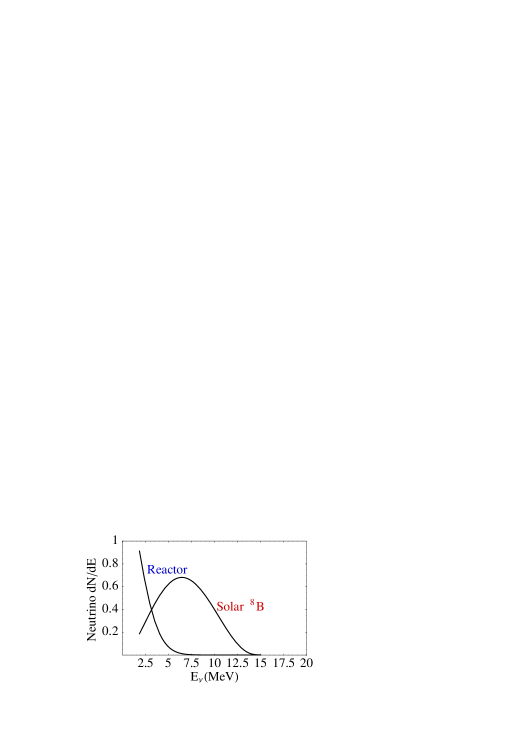
Figure 1: (Top) The reactor antineutrino and solar ${}^{8}B$ neutrino [26] fluxes. (Bottom). Upper limits on solar antineutrino conversion probabilities (from Ref.[17]).

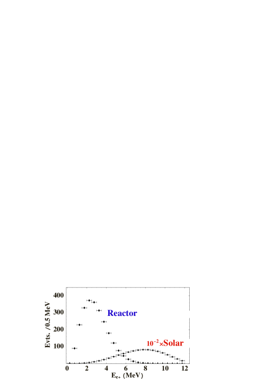
Figure 2: The KamLAND expected positron spectra in absence of oscillations coming from reactor antineutrinos (normalized to three years of data taking). The “solar” positron spectrum is obtained assuming the shape of the ${}^{8}B$ neutrino flux and a total normalization $10^{-2}\times\Phi({}^{8}B)$ (that is, an overall $\nu_{e}-\overline{\nu}_{e}$ conversion probability $\overline{P}\sim 1\%$).

References

- [1] Q. R. Ahmad et al. [SNO Collaboration], Phys. Rev. Lett. 89, 011302 (2002) [arXiv:nucl-ex/0204009].
- [2] Q. R. Ahmad et al. [SNO Collaboration], Phys. Rev. Lett. 89, 011301 (2002) [arXiv:nucl-ex/0204008].
- [3] ’How to use recent SNO results’,http://www.sno.phy.queensu.ca/
- [4] P. Aliani, V. Antonelli, R. Ferrari, M. Picariello and E. Torrente-Lujan, arXiv:hep-ph/0205053. P. Aliani, V. Antonelli, M. Picariello and E. Torrente-Lujan, Nucl. Phys. B634 (2002) 393-409. arXiv:hep-ph/0111418. P. Aliani, V. Antonelli, M. Picariello and E. Torrente-Lujan, Nucl. Phys. Proc. Suppl. 110, 361 (2002) [arXiv:hep-ph/0112101].
- [5] A. Strumia, C. Cattadori, N. Ferrari and F. Vissani, arXiv:hep-ph/0205261. A. Strumia and F. Vissani, JHEP 0111, 048 (2001)[arXiv:hep-ph/0109172].
- [6] A. Bandyopadhyay, S. Choubey, S. Goswami and D. P. Roy, Phys. Lett. B 540, 14 (2002) [arXiv:hep-ph/0204286].
- [7] V. Barger, D. Marfatia, K. Whisnant and B. P. Wood, Phys. Lett. B 537, 179 (2002) [arXiv:hep-ph/0204253].
- [8] S. Pascoli and S. T. Petcov, arXiv:hep-ph/0205022.
- [9] P. C. de Holanda and A. Y. Smirnov, arXiv:hep-ph/0205241.
- [10] J. N. Bahcall, M. C. Gonzalez-Garcia and C. Pena-Garay, arXiv:hep-ph/0204314.
- [11] R. Foot and R. R. Volkas, arXiv:hep-ph/0204265.
- [12] P. Aliani, V. Antonelli, R. Ferrari, M. Picariello and E. Torrente-Lujan, arXiv:hep-ph/0206308. E. Torrente-Lujan, arXiv:hep-ph/9902339. S. Khalil and E. Torrente-Lujan, J. Egyptian Math. Soc. 9 (2001) 91 [arXiv:hep-ph/0012203].
- [13] E. Torrente-Lujan, Prepared for 2nd ICRA Network Workshop: The Chaotic Universe: Theory, Observations, Computer Experiments, Rome, Italy, 1-5 Feb 1999. E. Torrente-Lujan, arXiv:hep-ph/9912225. E. Torrente-Lujan, Phys. Rev. D 59, 093006 (1999) [arXiv:hep-ph/9807371]. E. Torrente-Lujan, Phys. Rev. D 59, 073001 (1999) [arXiv:hep-ph/9807361]. E. Torrente-Lujan, arXiv:hep-ph/9602398. V. B. Semikoz and E. Torrente-Lujan, Nucl. Phys. B 556, 353 (1999) [arXiv:hep-ph/9809376].
- [14] E. Torrente-Lujan, Phys. Lett. B 441, 305 (1998) [arXiv:hep-ph/9807426].
- [15] A. Piepke [kamLAND collaboration], Nucl. Phys. Proc. Suppl. 91, 99 (2001)
- [16] J. Shirai, “Start of Kamland”, talk given at Neutrino 2002, XXth International Conference on Neutrino Physics and Astrophysics, May 2002, Munich. Transparencies can be obtained from http://neutrino2002.ph.tum.de. See also: P. Alivisatos et al., STANFORD-HEP-98-03.
- [17] E. Torrente-Lujan, Nucl. Phys. Proc. Suppl. 87, 504 (2000). E. Torrente-Lujan, Phys. Lett. B 494, 255 (2000) [arXiv:hep-ph/9911458].
- [18] M. Apollonio et al., CHOOZ Coll., Phys. Lett. B 466, 415 (1999)
- [19] M. Apollonio et al. (CHOOZ coll.), hep-ex/9907037, Phys. Lett. B 466 (1999) 415. M. Apollonio et al., Phys. Lett. B 420 (1998) 397. F. Boehm et al.,Phys. Rev. D62 (2000) 072002 [hep-ex/0003022].
- [20] Y. F. Wang [Palo Verde Collaboration], Int. J. Mod. Phys. A 16S1B, 739 (2001); F. Boehm et al., Phys. Rev. D 64, 112001 (2001) [arXiv:hep-ex/0107009].
- [21] L. De Braeckeleer [KamLAND Collaboration], Nucl. Phys. Proc. Suppl. 87 (2000) 312. J. Shirai, “Kamioka Liquid Scintillator Anti-Neutrino Detector”, Neutrino2002, May 25-30, Munich, Germany. A. Suzuki [KamLAND Collaboration], Nucl. Phys. Proc. Suppl. 77 (1999) 171.
- [22] J. Busenitz et al. (US KamLand Coll). proposal for US Participation in KamLand. March 1999 (Unpublished).
- [23] K. S. Hirata et al. [Kamiokande-II Collaboration], Phys. Lett. B 280, 146 (1992). T. Toshito [SuperKamiokande Collaboration], arXiv:hep-ex/0105023; Y. Fukuda et al. [Super-Kamiokande Collaboration], Phys. Rev. Lett. 81, 1562 (1998) [arXiv:hep-ex/9807003]; R. Becker-Szendy et al., Nucl. Phys. Proc. Suppl. 38, 331 (1995); M. Sanchez [Soudan-2 Collaboration], Int. J. Mod. Phys. A 16S1B, 727 (2001); M. Ambrosio et al. [MACRO Collaboration], arXiv:hep-ex/0206027.
- [24] P. Aliani, V. Antonelli, M. Picariello and E. Torrente-Lujan, arXiv:hep-ph/0207348. P. Aliani, V. Antonelli, R. Ferrari, M. Picariello and E. Torrente-Lujan, arXiv:hep-ph/0205061.
- [25] V. Barger, D. Marfatia and K. Whisnant, arXiv:hep-ph/0106207.
- [26] J. N. Bahcall, M. H. Pinsonneault and S. Basu, Astrophys. J. 555, 990 (2001) [arXiv:astro-ph/0010346].
- [27] H. Murayama and A. Pierce, Phys. Rev. D 65 (2002) 013012 [arXiv:hep-ph/0012075].
- [28] P. Vogel and J. F. Beacom, Phys. Rev. D 60, 053003 (1999) [arXiv:hep-ph/9903554].
- [29] G. Zacek et al. Phys. Rev. D34,9 (1986)2621.
- [30] F. Reines, R. M. Woods, Phys. Rev. Lett. 14 (1965) 20.
- [31] D. H. Wilkinson, Nucl. Phys. A377, 474 (1982).
- [32] K. Hagiwara et al., Phys. Rev. D 66 (2002) 010001