Forward–Backward Asymmetry in $B\rightarrow X_{s}\ell^{+}\ell^{-}$

at the NNLL Level

A. Ghinculov,^a, T. Hurth,^b, G. Isidori,^b,c Y.-P. Yao^d,1

^a Department of Physics and Astronomy
UCLA, Los Angeles CA 90095-1547, USA
^b Theoretical Physics Division, CERN, CH-1211 Geneva 23, Switzerland
^c INFN, Laboratori Nazionali di Frascati, I-00044 Frascati, Italy
^d Randall Laboratory of Physics
University of Michigan, Ann Arbor MI 48109-1120, USA

Abstract

We report the results of a new calculation of soft-gluon corrections in $B\rightarrow X_{s}\ell^{+}\ell^{-}$ decays. In particular, we present the first calculation of bremsstrahlung and corresponding virtual terms to the lepton forward–backward asymmetry, which allows us to systematically include all contributions to this observable beyond the lowest non-trivial order. The new terms are important, for instance the position of the zero of the asymmetry receives corrections of $O(10\%)$. Using a different method, we also provide an independent check of recently published results on bremsstrahlung and infrared virtual corrections to the dilepton-invariant mass distribution.

1 Introduction

Flavour-changing neutral-current (FCNC) processes are a very useful tool to understand the nature of physics beyond the Standard Model (SM). The stringent bounds obtained from $B\rightarrow X_{s}\gamma$ on various non-standard scenarios (see e.g. [1, 2, 3, 4]) are a clear example of the importance of theoretically clean FCNC observables in discriminating new-physics models.

Generally, inclusive rare decay modes of the $B$ meson are theoretically clean observables. For instance the decay width $\Gamma(B\to X_{s}\gamma)$ is well approximated by the partonic decay rate $\Gamma(b\to s\gamma)$, which can be analysed in renormalization-group-improved perturbation theory. Non-perturbative contributions play only a subdominant role and can be calculated in a model-independent way by using the heavy-quark expansion. The inclusive $B\rightarrow X_{s}\ell^{+}\ell^{-}$ transition, which is starting to be accessible at $B$ factories [5], represents a new source of theoretically clean observables, complementary to the $B\rightarrow X_{s}\gamma$ rate. In particular, kinematic observables such as the invariant dilepton mass spectrum and the forward–backward (FB) asymmetry in $B\rightarrow X_{s}\ell^{+}\ell^{-}$ provide additional clean information on short-distance couplings not accessible in $B\rightarrow X_{s}\gamma$ [6].

Non-perturbative corrections to $B\rightarrow X_{s}\ell^{+}\ell^{-}$ scaling with $1/m_{b}^{2}$ and $1/m_{c}^{2}$ can be calculated quite analogously to those entering the $B\rightarrow X_{s}\gamma$ rate [7, 8, 9, 10]. Here the $c\bar{c}$ resonances represent a more serious problem since, for specific values of the dilepton invariant mass, $c\bar{c}$ states can be produced on shell. However, these resonances can be removed by appropriate kinematic cuts in the invariant mass spectrum. In the perturbative window, namely when $m_{\ell^{+}\ell^{-}}\stackrel{{\scriptstyle<}}{{{}_{\sim}}}~{}m_{b}/2$, theoretical predictions for the invariant mass spectrum are dominated by the purely perturbative contributions, and a theoretical precision comparable with the one reached in the decay $B\rightarrow X_{s}\gamma$ is possible. The $B$ factories will soon provide statistics and resolution needed for the measurements of $B\rightarrow X_{s}\ell^{+}\ell^{-}$ kinematic distributions. Precise theoretical estimates of the SM expectations are therefore needed in order to perform new significant tests of flavour physics.

In this paper we complete one important step of this program: we present a new calculation of QCD-bremsstrahlung and the corresponding virtual corrections in $B\rightarrow X_{s}\ell^{+}\ell^{-}$. This effect has already been evaluated in Refs. [11, 12] for the dilepton invariant-mass spectrum. Here we perform the calculation using a different technique, namely using a full dimensional regularization of infrared divergences (both soft and collinear ones). We anticipate that our results agree with those of [11, 12] for the dilepton invariant-mass distribution. Moreover, our technique allows us obtain the first computation of the soft-gluon (and corresponding virtual) corrections in the FB asymmetry: the missing ingredient needed for a systematic evaluation of this observable beyond the lowest non-trivial order. Our phenomenological analysis shows that these new contributions are rather important, for instance the position of the zero of the asymmetry receives corrections of $O(10\%)$.

The paper is organized as follows: in Section 2 we set up the framework of the calculation; we briefly review the status of the various ingredients needed for a systematic analysis of the partonic process $b\rightarrow s(g)\ell^{+}\ell^{-}$ in perturbation theory. In Section 3 we present the basic expressions needed to describe the spectrum and the FB asymmetry of $B\rightarrow X_{s}\ell^{+}\ell^{-}$ in the so-called next-to-next-to-leading logarithmic (NNLL) approximation. The details of the calculation, including a definition of the four-particle phase space and a discussion on the regularization scheme, which avoids any ambiguity due to the definition $\gamma_{5}$, are presented in Section 4. Section 5 contains a brief phenomenological analysis of our results, mainly focused on the determination of the zero of the FB asymmetry, and Section 6 a short summary.

2 Theoretical framework

Within inclusive $B$ decay modes such as $B\rightarrow X_{s}\gamma$ or $B\rightarrow X_{s}\ell^{+}\ell^{-}$, short-distance QCD corrections lead to a sizeable modification of the pure electroweak contribution, generating large logarithms of the form $\alpha_{s}^{n}(m_{b})\,\log^{m}(m_{b}/M_{\rm heavy})$, where $M_{\rm heavy}=O(M_{W})$ and $m\leq n$ (with $n=0,1,2,...$). A suitable framework to achieve the necessary resummations of these large logs is the construction of an effective low-energy theory with five quarks, obtained by integrating out the heavy degrees of freedom. With the help of renormalization-group (RG) techniques, one can then resum the series of leading logarithms (LL), next-to-leading logarithms (NLL), and so on:

$$\alpha_{s}^{n}(m_{b})\,\log^{n}(m_{b}/M)\quad[\mbox{LL}],\qquad\alpha_{s}^{n+1}(m_{b})\,\log^{n}(m_{b}/M)\quad[\mbox{NLL}]~{},\ldots$$ (2.1)

The effective five-quark low-energy Hamiltonian relevant to the partonic process $b\rightarrow s\ell^{+}\ell^{-}$ can be written as

$${\cal H}_{eff}=-\frac{4G_{F}}{\sqrt{2}}V_{ts}^{*}V_{tb}\,\sum{C_{i}(\mu,M_{\rm heavy})}\,\,\,{\cal O}_{i}(\mu)\,,$$ (2.2)

where

$$\begin{array}[]{rlrl}{\cal O}_{1}~{}=&\!\!(\bar{s}\gamma_{\mu}T^{a}P_{L}c)\,(\bar{c}\gamma^{\mu}T_{a}P_{L}b)\,,&{\cal O}_{2}~{}=&\!\!(\bar{s}\gamma_{\mu}P_{L}c)\,(\bar{c}\gamma^{\mu}P_{L}b)\,,\\[5.16663pt] {\cal O}_{3}~{}=&\!\!(\bar{s}\gamma_{\mu}P_{L}b)\sum_{q}(\bar{q}\gamma^{\mu}q)\,,&{\cal O}_{4}~{}=&\!\!(\bar{s}\gamma_{\mu}T^{a}P_{L}b)\sum_{q}(\bar{q}\gamma^{\mu}T_{a}q)\,,\\[5.16663pt] {\cal O}_{5}~{}=&\!\!(\bar{s}\gamma_{\mu}\gamma_{\nu}\gamma_{\rho}P_{L}b)\sum_{q}(\bar{q}\gamma^{\mu}\gamma^{\nu}\gamma^{\rho}q)\,,&{\cal O}_{6}~{}=&\!\!(\bar{s}\gamma_{\mu}\gamma_{\nu}\gamma_{\rho}T^{a}P_{L}b)\sum_{q}(\bar{q}\gamma^{\mu}\gamma^{\nu}\gamma^{\rho}T_{a}q)\,,\\[8.61108pt] \widetilde{{\cal O}}_{7}~{}=&\!\!\displaystyle{\frac{e}{16\pi^{2}}}\,\overline{m}_{b}(\mu)\,(\bar{s}\sigma^{\mu\nu}P_{R}b)\,F_{\mu\nu}\,,&\widetilde{{\cal O}}_{8}~{}=&\!\!\displaystyle{\frac{g_{s}}{16\pi^{2}}}\,\overline{m}_{b}(\mu)\,(\bar{s}\sigma^{\mu\nu}T^{a}P_{R}b)\,G^{a}_{\mu\nu}\,,\\[8.61108pt] \widetilde{{\cal O}}_{9}~{}=&\!\!\displaystyle{\frac{e^{2}}{16\pi^{2}}}\,(\bar{s}\gamma_{\mu}P_{L}b)\,(\bar{\ell}\gamma^{\mu}\ell)\,,&\widetilde{{\cal O}}_{10}~{}=&\!\!\displaystyle{\frac{e^{2}}{16\pi^{2}}}\,(\bar{s}\gamma_{\mu}P_{L}b)\,(\bar{\ell}\gamma^{\mu}\gamma_{5}\ell)\end{array}$$ (2.3)

define the complete set of relevant dimension-6 operators and $C_{i}(\mu,M_{\rm heavy})$ the corresponding Wilson coefficients.

Within this framework, QCD corrections are twofold: corrections related to the Wilson coefficients, and those related to the matrix elements of the various operators, both evaluated at the low-energy scale $\mu\approx m_{b}$. As the heavy fields are integrated out, the top-quark-, $W$-, and $Z$-mass dependence is contained in the initial conditions of the Wilson coefficients, determined by a matching procedure between full and effective theory at the high scale (Step 1). By means of RG equations, the $C_{i}(\mu,M_{\rm heavy})$ are then evolved at the low scale (Step 2). Finally, the QCD corrections to the matrix elements of the operators are evaluated at the low scale (Step 3).

Compared with the effective Hamiltonian relevant to $b\to s\gamma$, Eq. (2.3) contains the $O(\alpha_{\rm em})$ additional operators $\widetilde{{\cal O}}_{9}$ and $\widetilde{{\cal O}}_{10}$. Moreover, it turns out that the first large logarithm of the form $\log(m_{b}/M_{W})$ arises already without gluons, because the operator ${\cal O}_{2}$ mixes into $\widetilde{{\cal O}}_{9}$ at one loop. This possibility, which has no equivalent in the $b\to s\gamma$ case, leads to the following ordering of contributions to the decay amplitude

$$\left[\alpha_{\rm em}\,\log(m_{b}/M)\right]\,\alpha_{s}^{n}(m_{b})\,\log^{n}(m_{b}/M)\qquad[\mbox{LL}]~{},$$

$$\left[\alpha_{\rm em}\,\log(m_{b}/M)\right]\,\alpha_{s}^{n+1}(m_{b})\,\log^{n}(m_{b}/M)\quad[\mbox{NLL}]~{},\ldots$$ (2.4)

Technically, to perform the resummation, it is convenient to transform these series into the standard form (2.1). This can be achieved by redefining magnetic, chromomagnetic and lepton-pair operators as follows [13, 14]:

$${\cal O}_{i}=\frac{16\pi^{2}}{g_{s}^{2}}\widetilde{{\cal O}}_{i}~{},\quad C_{i}=\frac{g_{s}^{2}}{(4\pi)^{2}}\widetilde{C}_{i}~{},\quad\quad(i=7,...,10).$$ (2.5)

This redefinition enables one to proceed in the standard way, or as in $b\to s\gamma$, in the three calculational steps discussed above [13, 14]. At the high scale, the Wilson coefficients can be computed at a given order in perturbation theory and expanded in powers of $\alpha_{s}$:

$$C_{i}=C^{(0)}_{i}+\frac{\alpha_{s}}{(4\pi)}C^{(1)}_{i}+\frac{\alpha_{s}^{2}}{(4\pi)^{2}}C^{(2)}_{i}+...$$ (2.6)

Obviously, the Wilson coefficients of the new operators ${\cal O}_{7-10}$ at the high scale start at order $\alpha_{s}$ only. Then the anomalous-dimension matrix has the canonical expansion in $\alpha_{s}$ and starts with a term proportional to $\alpha_{s}$:

$${\gamma}=\frac{\alpha_{s}}{4\pi}{\gamma}^{(0)}+\frac{\alpha_{s}^{2}}{(4\pi)^{2}}{\gamma}^{(1)}+\frac{\alpha_{s}^{3}}{(4\pi)^{3}}{\gamma}^{(2)}+...$$ (2.7)

In particular, after the reshufflings in (2.5) the one-loop mixing of the operator ${\cal O}_{2}$ with ${\cal O}_{9}$ appears formally at order $\alpha_{s}$.

The last of the three steps, however, requires some care: among the operators with a non-vanishing tree-level matrix element, only ${\cal O}_{9}$ has a non-vanishing coefficient at the LL level. Therefore, at this level, only the tree-level matrix element of this operator ($\langle{\cal O}_{9}\rangle$) has to be included. At NLL accuracy the QCD one-loop contributions to $\langle{\cal O}_{9}\rangle$, the tree-level contributions to $\langle{\cal O}_{7}\rangle$ and $\langle{\cal O}_{10}\rangle$, and the electroweak one-loop matrix elements of the four-quark operators have to be calculated. Finally, at NNLL precision, one should in principle take into account the QCD two-loop corrections to $\langle{\cal O}_{9}\rangle$, the QCD one-loop corrections to $\langle{\cal O}_{7}\rangle$ and $\langle{\cal O}_{10}\rangle$, and the QCD corrections to the electroweak one-loop matrix elements of the four-quark operators.

Let us briefly review the present status of these perturbative contributions to decay rate and FB asymmetry of $B\to X_{s}\ell^{+}\ell^{-}$: the complete NLL contributions to the decay amplitude can be found in [13, 14]. Since the LL contribution to the rate turns out to be numerically rather small, NLL terms represent an $O(1)$ correction to this observable. On the other hand, since a non-vanishing FB asymmetry is generated by the interference of vector ($\sim{\cal O}_{7,9}$) and axial-vector ($\sim{\cal O}_{10}$) leptonic currents, the LL amplitude leads to a vanishing result and NLL terms represent the lowest non-trivial contribution to this observable.

For these reasons, a computation of NNLL terms in $B\to X_{s}\ell^{+}\ell^{-}$ is needed if we aim at the same numerical accuracy as achieved by the NLL analysis of $B\to X_{s}\gamma$ [15]. Large parts of the latter can be taken over and used in the NNLL calculation of $B\to X_{s}\ell^{+}\ell^{-}$. However, this is not the full story. In particular, the bremsstrahlung corrections presented in this paper for the first time are a crucial ingredient, necessary for a complete evaluation of the FB asymmetry to NNLL precision. And in the case of the differential rate, the full NNLL enterprise is still not complete:

[Step 1] The full computation of initial conditions to NNLL precision has been presented in Ref. [16]. The authors did the two-loop matching for all the operators relevant to $b\to s\ell^{+}\ell^{-}$ (including a confirmation of the $b\to s\gamma$ NLL matching results of [17, 18]). The inclusion of this NNLL contribution removes the large matching scale uncertainty (around $16\%$) of the NLL calculation of the $b\to s\ell^{+}\ell^{-}$ decay rate.

[Step 2] Thanks to the reshufflings of the LL series, most of the NNLL contributions to the anomalous-dimension matrix can be derived from the NLL analysis of $b\to s\gamma$. In particular the three-loop mixing of the four-quark operators ${\cal O}_{1-6}$ into ${\cal O}_{7}$ and ${\cal O}_{8}$ can be taken over from Ref. [15]. The only missing piece for a full NNLL analysis of the $b\rightarrow s\ell^{+}\ell^{-}$ decay rate is the three-loop mixing of the four-quark operators into ${\cal O}_{9}$. In [16] an estimate was made, which suggests that the numerical influence of these missing NNLL contributions on the branching ratio of $b\rightarrow s\ell^{+}\ell^{-}$ is small. Interestingly, since the FB asymmetry has no contributions proportional to $|\langle{\cal O}_{9}\rangle|^{2}$, this missing term is not needed for a NNLL analysis of this observable.

[Step 3] Within the $B\rightarrow X_{s}\gamma$ calculation at NLL, the two-loop matrix elements of the four-quark operator ${\cal O}_{2}$ for an on-shell photon were calculated in [19] and quite recently confirmed in [20]. An independent numerical check of these results has been performed and will be presented in [21]. This calculation was extended in [11] to the case of an off-shell photon (for small squared dilepton mass), which corresponds to a NNLL contribution relevant to the decay $B\rightarrow X_{s}\ell^{+}\ell^{-}$. In the dilepton spectrum, this calculation reduces the error corresponding to the uncertainty of the low-scale dependence from $\pm 13\%$ down to $\pm 6.5\%$. This step also includes the bremsstrahlung and virtual contributions that are discussed in the present paper.
In principle, a complete NNLL calculation of the $B\rightarrow X_{s}\ell^{+}\ell^{-}$ rate would require also the calculation of the renormalization-group-invariant two-loop matrix element of the operator ${\cal O}_{9}$. Similarly to the missing piece of the anomalous-dimension matrix, also this (scale-independent) contribution does not enter the FB asymmetry at NNLL accuracy.

3 Basic expressions

We normalize all the observables by the semileptonic decay rate in order to reduce the uncertainties due to bottom quark mass and CKM angles:

$$\Gamma[b\to X_{c}e\bar{\nu}_{e}]=\frac{G_{F}^{2}m_{b}^{5}}{192\pi^{3}}|V_{cb}|^{2}f(z)\kappa(z)~{}.$$ (3.1)

Here $z=m_{c}^{2}/m_{b}^{2}$ ($m_{b,c}$ denote pole quark masses), $f(z)=1-8z+8z^{3}-z^{4}-12z^{2}\ln z$ is the phase-space factor and

$$\kappa(z)=1-\frac{2\alpha_{s}(m_{b})}{3\pi}\frac{h(z)}{f(z)}$$ (3.2)

takes into account QCD corrections (the function $h(z)$ has been given analytically in [22] and is quoted in the appendix). The normalized dilepton invariant mass spectrum is then defined as

$$R(s)=\frac{\frac{d}{ds}\Gamma(B\to X_{s}\ell^{+}\ell^{-})}{\Gamma(B\to X_{c}e\bar{\nu})}~{},$$ (3.3)

where $s=(p_{\ell^{+}}+p_{\ell^{-}})^{2}/m_{b}^{2}$. The other important observable is the forward–backward lepton asymmetry:

$$A_{\rm FB}(s)=\frac{1}{\Gamma(B\to X_{c}e\bar{\nu})}\int_{-1}^{1}d\cos\theta_{\ell}~{}\frac{d^{2}\Gamma(B\to X_{s}\ell^{+}\ell^{-})}{ds~{}d\cos\theta_{\ell}}\mbox{sgn}(\cos\theta_{\ell})~{},$$ (3.4)

where $\theta_{\ell}$ is the angle between $\ell^{+}$ and $B$ momenta in the dilepton centre-of-mass frame. It was shown in [8] that $A_{\rm FB}(s)$ is identical to the energy asymmetry introduced in [23].

Following closely — but not exactly — the notation of Refs. [11, 12], we present here some useful formulae that allow us to systematically take into account corrections beyond the NLL level for the partonic contributions to these two observables:

$$R(s)=\frac{\alpha_{\rm em}^{2}}{4\pi^{2}}\left|\frac{V_{tb}^{*}V_{ts}}{V_{cb}}\right|^{2} \!\!\!\!\!\!\!\!\frac{(1-s)^{2}}{f(z)\kappa(z)}\left\{4\left(1+\frac{2}{s}\right)|C^{\rm new}_{7}(s)|^{2}\left(1+\frac{\alpha_{s}}{\pi}\tau_{77}(s)\right)\right.$$ (3.5)

$$+(1+2s)\left[|C^{\rm new}_{9}(s)|^{2}+|C^{\rm new}_{10}(s)|^{2}\right]\left(1+\frac{\alpha_{s}}{\pi}\tau_{99}(s)\right)$$

$$\left.+12\,\mbox{Re}\left[C^{\rm new}_{7}(s)C^{\rm new}_{9}(s)^{*}\right]\left(1+\frac{\alpha_{s}}{\pi}\tau_{79}(s)\right)+\frac{\alpha_{s}}{\pi}\delta_{R}(s)\right\}~{},\qquad$$

$$A_{\rm FB}(s)=-\frac{3\alpha_{\rm em}^{2}}{4\pi^{2}}\left|\frac{V_{tb}^{*}V_{ts}}{V_{cb}}\right|^{2} \!\!\!\!\!\!\!\!\frac{(1-s)^{2}}{f(z)\kappa(z)}\left\{s\,\mbox{Re}\left[C^{\rm new}_{10}(s)^{*}C^{\rm new}_{9}(s)\right]\left(1+\frac{\alpha_{s}}{\pi}\tau_{910}(s)\right)\right.$$ (3.6)

$$\left.+2\,\mbox{Re}\left[C^{\rm new}_{10}(s)^{*}C^{\rm new}_{7}(s)\right]\left(1+\frac{\alpha_{s}}{\pi}\tau_{710}(s)\right)+\frac{\alpha_{s}}{\pi}\delta_{\rm FB}(s)\right\}~{}.$$

With respect to Refs. [11, 12], we have introduced a new set of effective coefficients, defined as

$$C^{\rm new}_{7}(s) = \left(1+\frac{\alpha_{s}}{\pi}\sigma_{7}(s)\right)\widetilde{C}_{7}^{\rm eff}-\frac{\alpha_{s}}{4\,\pi}\left[C_{1}^{(0)}F_{1}^{(7)}(s)+C_{2}^{(0)}F_{2}^{(7)}(s)+\widetilde{C}^{\rm eff(0)}_{8}F_{8}^{(7)}(s)\right]$$

$$C^{\rm new}_{9}(s) = \left(1+\frac{\alpha_{s}}{\pi}\sigma_{9}(s)\right)\widetilde{C}_{9}^{\rm eff}(s)-\frac{\alpha_{s}}{4\,\pi}\left[C_{1}^{(0)}F_{1}^{(9)}(s)+C_{2}^{(0)}F_{2}^{(9)}(s)+\widetilde{C}_{8}^{\rm eff(0)}F_{8}^{(9)}(s)\right]$$

$$C^{\rm new}_{10}(s) = \left(1+\frac{\alpha_{s}}{\pi}\sigma_{9}(s)\right)\widetilde{C}^{\rm eff}_{10}~{}.$$ (3.7)

The $C^{\rm new}_{i}$ have the advantage of encoding all dominant matrix-element corrections, which leads to an explicit $s$ dependence in all of them.

As we shall illustrate in detail in the next section, the terms $\sigma_{i}(s)$ take into account universal $O(\alpha_{s})$ bremsstrahlung and the corresponding infrared (IR) virtual corrections proportional to the tree-level matrix elements of ${\cal O}_{7-10}$. The remaining (finite) non-universal bremsstrahlung and IR virtual corrections are encoded in rate and FB asymmetry through $\tau_{i}(s)$ and $\delta_{R,{\rm FB}}(s)$. Analytic and numerical results for the $\tau_{i}(s)$ and the $\sigma_{i}(s)$ will be presented later on. Here we simply note that the $\sigma_{i}(s)$ are defined in order to take into account the truly soft component of the radiation, which diverges at the $s\to 1$ boundary of the phase space. With such definition of the $\sigma_{i}(s)$, the additional finite terms $\tau_{i}(s)$ are rather small all over the phase space and particularly for large values of $s$ ($|\tau_{i}(s)|<0.5$ for $s>0.3$). Substantially smaller are the bremsstrahlung corrections not related to ${\cal O}_{7-10}\otimes{\cal O}_{7-10}$, which are encoded in $\delta_{R,{\rm FB}}(s)$. A complete evaluation of $\delta_{R}(s)$ can be found in [12], where this effect is shown to be at the $O(1\%)$ level.

The other explicit $O(\alpha_{s})$ terms in (3.7) are due to virtual corrections that are infrared-safe. In particular, the two-loop functions $F_{1,2}^{(7,9)}$ and the one-loop functions $F_{8}^{(7),(9)}$ correspond to virtual corrections to ${\cal O}_{1,2}$ and ${\cal O}_{8}$, respectively. These functions have been computed in Ref. [11] for small $s$. The coefficients $\widetilde{C}^{\rm eff}_{7-10}$, including the one-loop matrix-element contributions of ${\cal O}_{1-6}$ are defined in close analogy with Ref. [14] and are reported in the appendix as a function of the true Wilson coefficients $C_{i}$. Finally, explicit expressions for the latter, evolved down at the low-energy scale, can be found in [16].

By means of expressions (3.5) and (3.6), we can more easily discuss the organization of the perturbative expansion for the two observables. According to the arguments in Section 2, the formally leading terms are obtained by setting $C^{\rm new}_{7}=C^{\rm new}_{10}=0$, neglecting $\tau_{i}$ and $\delta_{i}$, and identifying $C^{\rm new}_{9}$ with the leading term of $\widetilde{C}_{9}^{\rm eff}$ [formally $O(1/\alpha_{s})$]. At this level $A_{\rm FB}(s)$ is clearly vanishing. At the NNL level, when $A_{\rm FB}(s)$ receives its first non-vanishing contribution, we should retain the interference of the $O(1/\alpha_{s})$ term in $C^{\rm new}_{9}$ with the leading $O(1)$ terms in $C^{\rm new}_{7,10}$, as well as the subleading corrections in $|C^{\rm new}_{9}|^{2}$. Within this approach, the missing ingredients for a NNLL analysis of $A_{\rm FB}(s)$ are only $\sigma_{9}$ and $\tau_{910}$.

As anticipated, the standard LL expansion is numerically not well justified, since the formally-leading $O(1/\alpha_{s})$ term in $C^{\rm new}_{9}$ is much closer to an $O(1)$ term. For this reason, it has been proposed in Ref. [11] to use a different counting rule, where the $O(1/\alpha_{s})$ term of $C^{\rm new}_{9}$ is treated as $O(1)$. We also believe that this approach, although it cannot be consistently extended at higher orders, is well justified at the present status of the calculation. Within this approach, the three $C^{\rm new}_{i}$ and the two observables [$R(s)$ and $A_{\rm FB}(s)$] are all homogeneous quantities, starting with an $O(1)$ term. Then all $\sigma_{i}$, $\tau_{i}$ and $\delta_{i}$ functions are required for a next-to-leading order analysis of both $R(s)$ and $A_{\rm FB}(s)$.

4 Details of the calculation

In contrast to previous calculations of $B\to X_{s}\gamma$ and $B\to X_{s}\ell^{+}\ell^{-}$ matrix elements, we set $m_{s}=0$ and, following the approach of Ref. [24], we employ dimensional regularization to regulate all infrared singularities, including collinear divergences arising from the vanishing strange-quark mass.

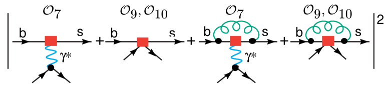
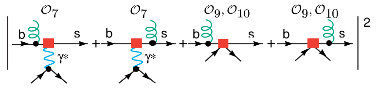
Figure 1: Virtual (up) and real (down) QCD corrections generating the terms $\tau_{i}$ and $\sigma_{i}$ in Eqs. (3.5)–(3.7). The boxes denote the insertion of ${\cal L}_{\rm eff}$ in (4.1).

The diagrams we need to compute are shown in Fig. 1, where the boxes denote the insertion of the following effective non-local Lagrangian

$${\cal L}_{\rm eff}=\kappa_{F}\left[\widetilde{C}_{9}^{\rm eff}\bar{s}\gamma_{\mu}P_{L}b~{}\bar{\ell}\gamma^{\mu}\ell+\widetilde{C}_{10}^{\rm eff}\bar{s}\gamma_{\mu}P_{L}b~{}\bar{\ell}\gamma^{\mu}\gamma_{5}\ell+\frac{m_{b}}{e}\widetilde{C}_{7}^{\rm eff}\bar{s}\sigma_{\mu\nu}P_{R}bF^{\mu\nu}\right]~{},$$ (4.1)

where

$$\kappa_{F}=\frac{\alpha_{\rm em}G_{F}V_{ts}^{*}V_{tb}}{\pi\sqrt{2}}$$ (4.2)

and, for simplicity, we have omitted to explicitly show the $s$ dependence of $\widetilde{C}_{9}^{\rm eff}$. Using (4.1) instead of the local Hamiltonian in (2.2), we can easily take into account the (two-loop) IR-divergent contributions of four-quark operators, whose one-loop $b\to s\ell^{+}\ell^{-}$ matrix element is encoded in the non-local coefficients $\widetilde{C}_{i}^{\rm eff}$ [11] (see appendix).

4.1 Virtual corrections

The amplitude for the three-body process $b(p)\to s(p_{s})\ell^{+}(p_{1})\ell^{-}(p_{2})$ can be written as

$${\cal A}_{[3]} = \frac{2\kappa_{F}}{m_{b}}\left\{\bar{s}P_{R}\left[m_{b}\gamma^{\mu}A(s)+(p^{\mu}+p_{s}^{\nu})B(s)+O(q^{\mu})\right]b\bar{\ell}\gamma_{\mu}\ell\right.$$ (4.3)

$$\qquad\left.+\bar{s}P_{R}\left[m_{b}\gamma^{\mu}A^{\prime}(s)+(p^{\mu}+p_{s}^{\nu})B^{\prime}(s)+O(q^{\mu})\right]b\bar{\ell}\gamma_{\mu}\gamma_{5}\ell\right\}~{},\$$

where $q=p_{1}+p_{2}$ and, at the tree level,

$$A^{(0)}=\frac{1}{2}\widetilde{C}_{9}^{\rm eff}+\frac{1}{s}\widetilde{C}_{7}^{\rm eff}~{},\qquad B^{(0)}=-\frac{1}{s}\widetilde{C}_{7}^{\rm eff}~{},\qquad A^{\prime(0)}=\frac{1}{2}\widetilde{C}_{10}^{\rm eff}~{},\qquad B^{\prime(0)}=0~{}.$$ (4.4)

Employing the same notation, and working in $d=4-2\epsilon$ dimensions, the renormalized virtual one-loop corrections in Fig. 1 are given by

$$A^{(1)} = \frac{\alpha_{s}}{3\pi}\Gamma(1+\epsilon)(1-s)^{-2\epsilon}\left(\frac{m_{b}^{2}}{4\pi}\right)^{-\epsilon}\left\{\widetilde{C}_{9}^{\rm eff}\left[-\frac{1}{2\epsilon^{2}}-\frac{5}{4\epsilon}-\mbox{Li}_{2}(s)-\frac{1+2s}{2s}\ln(1-s)-3\right]\right.$$

$$\qquad\left.+\frac{1}{s}\widetilde{C}_{7}^{\rm eff}\left[-\frac{1}{\epsilon^{2}}-\frac{5}{2\epsilon}-2\mbox{Li}_{2}(s)-3\ln(1-s)-10-8\ln\left(\frac{\mu}{m_{b}}\right)\right]+O(\epsilon)\right\}~{},$$

$$B^{(1)} = \frac{\alpha_{s}}{3\pi}\Gamma(1+\epsilon)(1-s)^{-2\epsilon}\left(\frac{m_{b}^{2}}{4\pi}\right)^{-\epsilon}\left\{\widetilde{C}_{9}^{\rm eff}\frac{1}{2s}\ln(1-s)\right.$$

$$\qquad\left.+\frac{1}{s}\widetilde{C}_{7}^{\rm eff}\left[\frac{1}{\epsilon^{2}}+\frac{5}{2\epsilon}+2\mbox{Li}_{2}(s)+\ln(1-s)+10+8\ln\left(\frac{\mu}{m_{b}}\right)\right]+O(\epsilon)\right\}~{},$$

$$A^{\prime(1)} = \frac{\alpha_{s}}{3\pi}\Gamma(1+\epsilon)(1-s)^{-2\epsilon}\left(\frac{m_{b}^{2}}{4\pi}\right)^{-\epsilon}\widetilde{C}_{10}^{\rm eff}\left[-\frac{1}{2\epsilon^{2}}-\frac{5}{4\epsilon}-\mbox{Li}_{2}(s)-\ln(1-s)\right.$$

$$\qquad\left.-3-\frac{1}{2s}\ln(1-s)+O(\epsilon)\right]~{},$$

$$B^{\prime(1)} = \frac{\alpha_{s}}{3\pi}\Gamma(1+\epsilon)(1-s)^{-2\epsilon}\left(\frac{m_{b}^{2}}{4\pi}\right)^{-\epsilon}\widetilde{C}_{10}^{\rm eff}\left[\frac{1}{2s}\ln(1-s)\right]~{}.$$ (4.5)

The above results include also self-energy corrections of the external legs, not explicitly shown in Fig. 1. Effectively, these contributions are included using on-shell renormalization conditions. For later comparison, we state here the corresponding on-shell wave-function renormalization constants for the external quark fields, where we explicitly separated ultraviolet (UV) and IR poles:

$$Z_{\psi}(m_{b}) = 1-\frac{\alpha_{s}}{4\pi}\frac{4}{3}\left(\frac{m_{b}^{2}}{\mu^{2}}\right)^{-\epsilon}\left(\frac{1}{\epsilon_{\rm UV}}+\frac{2}{\epsilon_{\rm IR}}+4\right)~{},$$

$$Z_{\psi}(m_{s}=0) = 1-\frac{\alpha_{s}}{4\pi}\frac{4}{3}\left(\frac{1}{\epsilon_{\rm UV}}-\frac{1}{\epsilon_{\rm IR}}\right)~{}.$$ (4.6)

Because of the conservation of vector and axial currents, UV divergences cancel out completely in the terms proportional to $\widetilde{C}_{9}^{\rm eff}$ and $\widetilde{C}_{10}^{\rm eff}$. On the other hand, UV divergences proportional to $\widetilde{C}_{7}^{\rm eff}$ have been eliminated by the on-shell mass counterterm $Z_{m_{b}}$ and by the ${\rm\overline{MS}}$ renormalization of the corresponding operator using the counterterm $Z_{77}$:

$$Z_{77} = 1+\frac{\alpha_{s}}{4\pi}\frac{16}{3}\frac{1}{\epsilon_{\rm UV}}~{},$$

$$Z_{m_{b}} = 1-\frac{\alpha_{s}}{4\pi}\frac{4}{3}\left(\frac{m_{b}^{2}}{\mu^{2}}\right)^{-\epsilon}\left(\frac{3}{\epsilon_{\rm UV}}+4\right)~{}.$$ (4.7)

After the UV renormalization has been performed, we suppress the $\mu$ dependence corresponding to the IR divergences in order to simplify the notation, as can be seen in Eq. (4.5).

Taking into account the full $d$-dimensional three-body phase space, virtual IR corrections to the rate and forward–backward asymmetry are obtained by means of Eqs. (4.3)–(4.5), isolating the $O(\alpha_{s})$ terms in

$${d\Gamma_{[3]}} = \frac{m_{b}}{2}\,\frac{d^{d-1}p_{s}}{(2\pi)^{d-1}2E_{s}}\,\frac{d^{d-1}q}{(2\pi)^{d-1}2q_{0}}\,(2\pi)^{d-1}\,\delta^{d}(p-p_{s}-q)\times$$ (4.8)

$$\times \frac{d^{d-1}p_{1}}{(2\pi)^{d-1}2E_{1}}\,\frac{d^{d-1}p_{2}}{(2\pi)^{d-1}2E_{2}}\,(2\pi)^{d}\,\delta^{d}(q-p_{1}-p_{2})\,ds\quad\frac{1}{2}\sum_{\rm spins}\frac{1}{3}\sum_{\rm colours}\left|{\cal A}_{[3]}\right|^{2}~{}$$

4.2 Bremsstrahlung corrections to $R(s)$

The matrix element of the four-body process $b(p)\to s(p_{s})g(k)\ell^{+}(p_{1})\ell^{-}(p_{2})$, squared, can in general be decomposed as

$$\frac{1}{2}\sum_{\rm spins}\frac{1}{3}\sum_{\rm colors}\left|{\cal A}_{[4]}\right|^{2}(s,y,x_{p},x_{s},x_{v})=H_{\mu\nu}^{S}L_{S}^{\mu\nu}+H_{\mu\nu}^{A}L_{A}^{\mu\nu}~{},$$ (4.9)

where $L_{S,A}^{\mu\nu}$ denote the leptonic tensors

$$L_{S}^{\mu\nu}={\rm tr}\left({/\!\!\!p}_{1}\gamma^{\mu}{/\!\!\!p}_{2}\gamma^{\nu}\right)\qquad{\rm and}\qquad L_{A}^{\mu\nu}={\rm tr}\left({/\!\!\!p}_{1}\gamma^{\mu}{/\!\!\!p}_{2}\gamma^{\nu}\gamma_{5}\right)~{},$$ (4.10)

and in addition to $s$ we have introduced the following kinematical variables

$$x_{p}=\frac{k\cdot p}{m^{2}_{b}}~{},\qquad x_{s}=\frac{k\cdot p_{s}}{m^{2}_{b}}~{},\qquad y=\frac{p\cdot(p_{1}-p_{2})}{m^{2}_{b}}~{},\qquad x_{v}=\frac{k\cdot(p_{1}-p_{2})}{m^{2}_{b}}~{}.$$ (4.11)

The asymmetric leptonic tensor $L_{A}^{\mu\nu}$ vanishes if averaged over the full leptonic phase space (symmetric in $p_{1}\leftrightarrow p_{2}$). On the other hand, in the case of $L_{S}^{\mu\nu}$ we can write

$$I^{\mu\nu}_{S} = (2\pi)^{d}\int\frac{d^{d-1}p_{1}}{(2\pi)^{d-1}2E_{1}}\int\frac{d^{d-1}p_{2}}{(2\pi)^{d-1}2E_{2}}\delta^{d}(q-p_{1}-p_{2})L_{S}^{\mu\nu}$$ (4.12)

$$= \frac{(1-\epsilon)(q^{2})^{-\epsilon}}{\pi^{\frac{1-2\epsilon}{2}}2^{3-4\epsilon}\Gamma\left(\frac{5}{2}-\epsilon\right)}\left(q^{\mu}q^{\nu}-q^{2}g^{\mu\nu}\right)~{}.$$

Since $I^{\mu\nu}_{S}$ depends only on $q$, the variables $y$ and $x_{v}$ do not appear in the calculation of the (symmetric) dilepton spectrum.

The explicit calculation of the real-emission diagrams in Fig. 1 leads to

$$\!\!\!\!\!\!\!\!\frac{1}{m_{b}^{2}}\left(q^{\mu}q^{\nu}-q^{2}g^{\mu\nu}\right)H_{\mu\nu}^{S}=\frac{16\pi}{3}\kappa_{F}^{2}\alpha_{s}\left\{\frac{}{}(1-s)\left[-\frac{1}{x_{p}^{2}}+\frac{1-s}{x_{p}x_{s}}-\frac{2}{x_{s}}+(1-\epsilon)\frac{2x_{p}}{x_{s}(1-s)}+\frac{2}{x_{p}}\right]\right.$$

$$\qquad\times\left[\frac{1+2s-2\epsilon s}{2}\left(\left|\widetilde{C}_{9}^{\rm eff}\right|^{2}+\left|\widetilde{C}_{10}^{\rm eff}\right|^{2}\right)+\frac{4+2s-4\epsilon}{s}\left|\widetilde{C}_{7}^{\rm eff}\right|^{2}+(6-4\epsilon)\mbox{Re}\left(\widetilde{C}_{7}^{\rm eff}\widetilde{C}_{9}^{\rm eff*}\right)\right]$$

$$\quad\qquad+\frac{x_{s}(1+2s)-2x_{p}}{x_{p}}\left(\left|\widetilde{C}_{9}^{\rm eff}\right|^{2}+\left|\widetilde{C}_{10}^{\rm eff}\right|^{2}\right)+\frac{4x_{s}(s-2+8x_{p})-8x_{p}(s+4)}{sx_{p}}\left|\widetilde{C}_{7}^{\rm eff}\right|^{2}$$

$$\left.\quad\qquad-\frac{4x_{s}+8x_{p}}{x_{p}}\mbox{Re}\left(\widetilde{C}_{7}^{\rm eff}\widetilde{C}_{9}^{\rm eff*}\right)+O(\epsilon)\right\}~{}.$$ (4.13)

Infrared singularities arise only by terms proportional to $1/x_{p}^{2}$ or $1/x_{s}$: for this reason only the $O(\epsilon)$ pieces proportional to these terms (between square brackets) have been explicitly shown. Taking into account the full $d$-dimensional four-body phase space, the radiative differential rate can be written as

$$\frac{d\Gamma_{[4]}}{ds} = \frac{m_{b}}{2}(2\pi)^{d-1}\int\frac{d^{d-1}p_{s}}{(2\pi)^{d-1}2E_{s}}\int\frac{d^{d-1}k}{(2\pi)^{d-1}2E_{g}}\int\frac{d^{d-1}q}{(2\pi)^{d-1}2q_{0}}\delta^{d}(p-p_{s}-k-q)I_{S}^{\mu\nu}H^{S}_{\mu\nu}$$ (4.14)

$$= \frac{C_{S}}{16\pi^{2}}s^{-\epsilon}(1-s)^{3-4\epsilon}\int_{0}^{1}dx(1-x)^{1-2\epsilon}x^{1-2\epsilon}\int_{0}^{1}d\omega(1-\omega)^{-\epsilon}\omega^{-\epsilon}$$

$$\times[1-x\omega(1-s)]^{-2+2\epsilon}\left[\frac{1}{m_{b}^{2}}\left(q^{\mu}q^{\nu}-q^{2}g^{\mu\nu}\right)H_{\mu\nu}^{S}\right]~{},\qquad\quad$$

where

$$C_{S}=\frac{(1-\epsilon)m_{b}^{5-6\epsilon}}{\pi^{2-3\epsilon}2^{9-10\epsilon}\Gamma\left(1-\epsilon\right)\Gamma\left(\frac{5}{2}-\epsilon\right)\Gamma\left(\frac{3}{2}-\epsilon\right)}~{}.$$ (4.15)

The integration variables in Eq. (4.14) are defined by

$$\omega=\frac{1}{2}(1-\cos\theta_{sk})~{},\qquad\qquad x=\frac{2p\cdot k}{m_{b}^{2}-q^{2}}~{},$$ (4.16)

where $\theta_{sk}$ is the angle between gluon and strange-quark momenta in the $B$ rest frame, so that

$$x_{p}(s,x)=\frac{x(1-s)}{2}~{},\qquad x_{s}(s,x,\omega)=\frac{x\omega(1-x)(1-s)^{2}}{2[1-x\omega(1-s)]}~{}.$$ (4.17)

Performing explicitly the integrals in $x$ and $\omega$ we obtain

$$\!\!\!\frac{d\Gamma_{[4]}}{ds}=\frac{\alpha_{s}}{3\pi}\kappa_{F}^{2}C_{S}s^{-\epsilon}(1-s)^{2-4\epsilon}$$

$$\ \times\left\{\left[\frac{2}{\epsilon^{2}}+\frac{5}{\epsilon}-4\mbox{Li}_{2}(s)-4\ln(s)\ln(1-s)-\pi^{2}+\frac{35}{2}+\frac{1}{1-s}-\frac{s(2-3s)}{(1-s)^{2}}\ln(s)\right]\right.$$

$$\ \ \ \times\left[\frac{1+2s-2\epsilon s}{2}\left(\left|\widetilde{C}_{9}^{\rm eff}\right|^{2}+\left|\widetilde{C}_{10}^{\rm eff}\right|^{2}\right)+\frac{4+2s-4\epsilon}{s}\left|\widetilde{C}_{7}^{\rm eff}\right|^{2}+(6-4\epsilon)\mbox{Re}\left(\widetilde{C}_{7}^{\rm eff}\widetilde{C}_{9}^{\rm eff*}\right)\right]\qquad$$

$$\qquad+\frac{s(4s^{2}+10s-4)\ln(s)-10s^{3}+7s^{2}+6s-3}{4(1-s)^{2}}\left(\left|\widetilde{C}_{9}^{\rm eff}\right|^{2}+\left|\widetilde{C}_{10}^{\rm eff}\right|^{2}\right)$$

$$\qquad+\frac{s(6s^{2}+24s-24)\ln(s)-19s^{3}+18s^{2}+15s-14}{3s(1-s)^{2}}\left|\widetilde{C}_{7}^{\rm eff}\right|^{2}$$

$$\qquad\left.-\frac{s(2s+12)\ln(s)-9s^{2}+4s+5}{(1-s)^{2}}\mbox{Re}\left(\widetilde{C}_{7}^{\rm eff}\widetilde{C}_{9}^{\rm eff*}\right)\right\}~{}.$$ (4.18)

In order to construct an IR-safe observable, $d\Gamma_{[4]}/ds$ has to be combined with the ${\cal O}(\alpha_{s})$ virtual corrections in the non-radiative process. The differential decay rate for the latter can be written as

$$\frac{d\Gamma_{[3]}}{ds} = \kappa_{F}^{2}C_{S}s^{-\epsilon}(1-s)^{2-2\epsilon}\Gamma(1-\epsilon)\left(\frac{m_{b}}{4\pi}\right)^{\epsilon}$$ (4.19)

$$\times \!\!\!\!\!\left\{2A^{2}[1+2s(1-\epsilon)]+4AB(1-s)+2B^{2}(1-s)^{2}+(A,B\leftrightarrow A^{\prime},B^{\prime})\right\}\qquad$$

in terms of the reduced amplitudes ($A,~{}B$) and ($A^{\prime},~{}B^{\prime}$) defined in (4.3). Using Eqs. (4.4)–(4.5) and isolating the ${\cal O}(\alpha_{s})$ terms we then obtain

$$\!\!\!\frac{d\Gamma^{(1)}_{[3]}}{ds}=\frac{\alpha_{s}}{3\pi}\kappa_{F}^{2}C_{S}s^{-\epsilon}(1-s)^{2-4\epsilon}\Gamma(1+\epsilon)\Gamma(1-\epsilon)$$

$$\ \times\left\{-\frac{1+2s-2\epsilon s}{2}\left(\left|\widetilde{C}_{9}^{\rm eff}\right|^{2}+\left|\widetilde{C}_{10}^{\rm eff}\right|^{2}\right)\left[\frac{2}{\epsilon^{2}}+\frac{5}{\epsilon}+4\mbox{Li}_{2}(s)+\frac{2+4s}{s}\ln(1-s)+12\right]\right.$$

$$\quad\ -\frac{4+2s-4\epsilon}{s}\left|\widetilde{C}_{7}^{\rm eff}\right|^{2}\left[\frac{2}{\epsilon^{2}}+\frac{5}{\epsilon}+4\mbox{Li}_{2}(s)+4\ln(1-s)+20+16\ln\left(\frac{\mu}{m_{b}}\right)\right]$$

$$\quad\ -(6-4\epsilon)\mbox{Re}\left(\widetilde{C}_{7}^{\rm eff}\widetilde{C}_{9}^{\rm eff*}\right)\left[\frac{2}{\epsilon^{2}}+\frac{5}{\epsilon}+4\mbox{Li}_{2}(s)+\frac{1+4s}{s}\ln(1-s)+16+8\ln\left(\frac{\mu}{m_{b}}\right)\right]$$

$$\left.\ +\frac{\ln(1-s)}{s}\left[(1-s)\left(\left|\widetilde{C}_{9}^{\rm eff}\right|^{2}+\left|\widetilde{C}_{10}^{\rm eff}\right|^{2}\right)-4(4-s)\left|\widetilde{C}_{7}^{\rm eff}\right|^{2}-2(1+2s)\mbox{Re}\left(\widetilde{C}_{7}^{\rm eff}\widetilde{C}_{9}^{\rm eff*}\right)\right]\right\}$$

(4.20)

It is straightforward to check that all divergences cancel in the sum of Eq. (4.18) and Eq. (4.20). Combining these two equations we can finally obtain explicit expression for the $\tau_{i}(s)$ and $\sigma_{i}(s)$ functions defined in Eq. (3.5).

As mentioned before, we define the universal functions $\sigma_{7,9}(s)$ such that the non-universal terms $\tau_{77}(s)$ and $\tau_{99}(s)$ vanish for $s\to 1$. This is because in the $s\to 1$ limit only the soft component of the radiation survives and, according to Low’s theorem, the latter gives rise to a correction proportional to the tree-level matrix. We then define

$$\sigma_{9}(s) = \sigma(s)+\frac{3}{2}~{},\qquad\qquad\sigma_{7}(s)\ =\ \sigma(s)+\frac{1}{6}-\frac{8}{3}\ln\left(\frac{\mu}{m_{b}}\right)~{},$$

$$\sigma(s) = -\frac{4}{3}\mbox{Li}_{2}(s)-\frac{2}{3}\ln(s)\ln(1-s)-\frac{2}{9}\pi^{2}-\ln(1-s)-\frac{2}{9}(1-s)\ln(1-s)~{}.\qquad$$ (4.21)

With this choice the $\tau_{i}(s)$ are given by

$$\tau_{77}(s) = -\frac{2}{9(2+s)}\left[2(1-s)^{2}\ln(1-s)+\frac{6s(2-2s-s^{2})}{(1-s)^{2}}\ln(s)+\frac{11-7s-10s^{2}}{(1-s)}\right]~{},$$

$$\tau_{99}(s) = -\frac{4}{9(1+2s)}\left[2(1-s)^{2}\ln(1-s)+\frac{3s(1+s)(1-2s)}{(1-s)^{2}}\ln(s)+\frac{3(1-3s^{2})}{1-s}\right]~{},$$

$$\tau_{79}(s) = -\frac{4(1-s)^{2}}{9s}\ln(1-s)-\frac{4s(3-2s)}{9(1-s)^{2}}\ln(s)-\frac{2(5-3s)}{9(1-s)}~{},$$ (4.22)

and all vanish at $s=1$.

These results are in complete agreement with those recently obtained by Asatrian et al. [11]. Indeed the $\omega_{i}(s)$ of Ref. [11] can be written as $\omega_{7}=\sigma_{7}+\tau_{77}/2$, $\omega_{9}=\sigma_{9}+\tau_{99}/2$, $\omega_{79}=(\sigma_{7}+\sigma_{9}+\tau_{79})/2$.

4.3 Virtual and bremsstrahlung corrections to $A_{\rm FB}(s)$

A use of naïve dimensional regularization is not allowed in the case of the forward–backward asymmetry because of the ambiguities arising for $d\not=4$ in the definition of $\gamma_{5}$ (or in the trace of $L_{A}^{\mu\nu}$); in the case of the decay rate, the problematic $\gamma_{5}$ contribution vanishes because of the $p_{1}\leftrightarrow p_{2}$ permutation symmetry of the leptonic phase space [see Eq. (4.12)]. To circumvent this problem, we employ the following regularization scheme: we treat the Dirac algebra of IR-divergent pieces strictly in four dimensions (dimensional reduction). This of course simplifies the calculation of the real emission, where only IR divergences appear, but it slightly complicates the virtual corrections, where UV divergences also occur. The latter, which do not involve any $\gamma_{5}$ ambiguity, are still computed in naïve dimensional regularization and renormalized as discussed at the beginning of this section. We stress that, at this level of the perturbative expansion, this hybrid regularization scheme is gauge invariant.

Within the virtual corrections we therefore need to strictly separate IR and UV divergences. As a result, the on-shell wave-function-renormalization factors given in Eqs. (4.1) within naïve dimensional regularization are partially changed. While the IR part of $Z_{\psi}(m_{b})$ is not modified, $Z_{\psi}(m_{s}=0)$ is different within our hybrid dimensional scheme:

$$Z_{\psi}(m_{b}) = 1-\frac{\alpha_{s}}{4\pi}\frac{4}{3}\left(\frac{\mu}{m}\right)^{2\epsilon}\left(\frac{1}{\epsilon_{\rm UV}}+\frac{2}{\epsilon_{\rm IR}}+4\right)~{},$$

$$Z_{\psi}(m_{s}=0) = 1-\frac{\alpha_{s}}{4\pi}\frac{4}{3}\left(\frac{1}{\epsilon_{\rm UV}}-\frac{1}{\epsilon_{\rm IR}}-1\right)~{}.$$ (4.23)

Being of pure UV nature, the other $Z$ factors remain unchanged. On the amplitude level, the change of $Z_{\psi}(m_{s}=0)$ turns out to be the only change of virtual corrections. Taking this effect into account, Eqs. (4.5) are modified as follows:

$$A^{(1)}_{D4} = A^{(1)}+\frac{\alpha_{s}}{3\pi}\Gamma(1+\epsilon)(1-s)^{-2\epsilon}\left(\frac{m_{b}^{2}}{4\pi}\right)^{-\epsilon}\left[\frac{1}{4}\widetilde{C}_{9}^{\rm eff}+\frac{1}{2s}\widetilde{C}_{7}^{\rm eff}\right]~{},$$

$$B^{(1)}_{D4} = B^{(1)}+\frac{\alpha_{s}}{3\pi}\Gamma(1+\epsilon)(1-s)^{-2\epsilon}\left(\frac{m_{b}^{2}}{4\pi}\right)^{-\epsilon}\left[-\frac{1}{2s}\widetilde{C}_{7}^{\rm eff}\right]~{},$$

$$A^{\prime(1)}_{D4} = A^{\prime(1)}+\frac{\alpha_{s}}{3\pi}\Gamma(1+\epsilon)(1-s)^{-2\epsilon}\left(\frac{m_{b}^{2}}{4\pi}\right)^{-\epsilon}\left[\frac{1}{4}\widetilde{C}_{9}^{\rm eff}\right]~{},\qquad B^{\prime(1)}_{D4}=B^{\prime(1)}~{}.\qquad$$ (4.24)

As a consistency check, we have explicitly verified that the finite corrections to $R(s)$, computed in the hybrid scheme, are exactly the same as in Eqs. (4.21)–(4.22). To this purpose, the bremsstrahlung term with four-dimensional Dirac algebra is obtained by neglecting all the $O(\epsilon)$ terms in Eq. (4.13).

The asymmetric part of the squared matrix element of the four-body process — relevant to $A_{\rm FB}(s)$ — computed with four-dimensional Dirac algebra, is given by

$$\frac{1}{m_{b}^{2}}H_{\mu\nu}^{A}L_{A}^{\mu\nu}~{} = \frac{128\pi}{3}\kappa_{F}^{2}\alpha_{s}\left\{y\left[-\frac{1}{x_{p}^{2}}+\frac{1-s}{x_{p}x_{s}}-\frac{2}{x_{s}}+\frac{2x_{p}}{x_{s}(1-s)}\right]\mbox{Re}\left[\widetilde{C}_{10}^{\rm eff*}\left(s\widetilde{C}_{9}^{\rm eff}+2\widetilde{C}_{7}^{\rm eff}\right)\right]\right.$$ (4.25)

$$+s\left[\frac{2yx_{p}-x_{v}(1-s)}{2x_{p}x_{s}(1-s)}(1-s-2x_{p})+\frac{y}{x_{p}}+\frac{x_{v}}{x_{p}^{2}}\right]\mbox{Re}\left(\widetilde{C}_{10}^{\rm eff*}\widetilde{C}_{9}^{\rm eff}\right)$$

$$+\frac{1}{s}\left[\frac{2yx_{p}-x_{v}(1-s)}{2x_{p}x_{s}(1-s)}\left(2s(1-s-2x_{p})+x_{p}(1-s)\right)+\frac{y}{x_{p}}(x_{s}+2s-2x_{p})\right.$$

$$\left.\left.\quad+\frac{x_{v}}{2x_{p}^{2}}\left(4s-2x_{s}x_{p}+(1-3s)x_{p}+2x_{p}^{2}\right)\right]\mbox{Re}\left(\widetilde{C}_{10}^{\rm eff*}\widetilde{C}_{7}^{\rm eff}\right)\right\}~{}.$$

As can be noted, $H_{\mu\nu}^{A}L_{A}^{\mu\nu}$ is linear in the leptonic asymmetric variables $y$ and $x_{v}$. The latter can be written as

$$y = -\cos\theta_{\ell}\left[\left(\frac{p\cdot q}{m_{b}^{2}}\right)^{2}-\frac{q^{2}}{m_{b}^{2}}\right]^{1/2},$$

$$x_{v} = y~{}\frac{p\cdot k}{m_{b}^{2}}\left[1+(p\cdot q)\frac{(p\cdot p_{s})\cos\theta_{sk}+(p\cdot k)}{(p\cdot q)^{2}-q^{2}m_{b}^{2}}+O(\sin\phi_{\ell})\right]~{},\qquad$$ (4.26)

where $\theta_{\ell}$ is the angle between $\ell^{+}$ and $B$ momenta in the dilepton centre-of-mass frame and $\phi_{\ell}$ the corresponding azimuthal angle. The integrals of $y$ and $x_{v}$ over the leptonic phase space, weighted by $\mbox{sgn}(\cos\theta_{\ell})$, can be expressed in terms of $s$ and the two integration variables $x$ and $\omega$ defined in Eq. (4.16):

$$\int\frac{d^{d-1}p_{1}}{2E_{1}}\!\!\!\!\!\!\!\! \!\!\!\!\int\frac{d^{d-1}p_{2}}{2E_{2}}\frac{\delta^{d}(q-p_{1}-p_{2})}{(2\pi)^{d-2}}\mbox{sgn}(\cos\theta_{\ell})\left\{\begin{array}[]{c}y\\ x_{v}\end{array}\right\}=\frac{(q^{2})^{-\epsilon}(1-\epsilon)^{-1}}{\pi^{1-\epsilon}2^{4-4\epsilon}\Gamma\left(1-\epsilon\right)}\left\{\begin{array}[]{c}{\overline{y}}(s,x,\omega)\\ {\overline{x}_{v}}(s,x,\omega)\end{array}\right\}$$ (4.31)

$${\overline{y}}(s,x,\omega)\!\! = \!\!-\frac{(1-s)\beta(s,x,\omega)}{2[1-x(1-s)\omega]}~{},$$

$${\overline{x}_{v}}(s,x,\omega)\!\! = \!\!{\overline{y}}x_{p}\left[1+(1+s-2x_{s})\frac{(1-s+2x_{s})(1-2\omega)+4\omega x_{p}}{(1-s)^{2}-4(1+s)x_{s}+4x_{s}^{2}}\right]~{},$$ (4.32)

where $x_{s,p}$ are given as in Eq. (4.17) and

$$\beta(s,x,\omega)=\sqrt{1-x\omega\left[4(1-x)+2x(1-s)(1-2\omega)+x^{2}\omega(1-s)(4-x(1-s))\right]}~{}.$$ (4.33)

Taking into account also the phase-space integration over the hadronic variables, the regularized bremsstrahlung contribution to the FB asymmetry can be written as

$$\frac{d\Gamma^{A}_{[4]}}{ds} = \int d\cos\theta_{\ell}~{}\frac{d^{2}\Gamma_{[4]}}{ds~{}d\cos\theta_{\ell}}\mbox{sgn}(\cos\theta_{\ell})=\frac{C_{A}}{16\pi^{2}}s^{-\epsilon}(1-s)^{3-4\epsilon}\int_{0}^{1}dx(1-x)^{1-2\epsilon}x^{1-2\epsilon}$$ (4.34)

$$\int_{0}^{1}d\omega(1-\omega)^{-\epsilon}\omega^{-\epsilon}[1-x\omega(1-s)]^{-2+2\epsilon}\left[\frac{1}{m_{b}^{2}}H_{\mu\nu}^{A}L_{A}^{\mu\nu}\right]_{y\to{\overline{y}}(s,x,\omega),x_{v}\to{\overline{x}_{v}}(s,x,\omega)}\quad\qquad$$

where

$$C_{A}=\frac{m_{b}^{5-6\epsilon}}{\pi^{\frac{5}{2}-3\epsilon}2^{10-10\epsilon}(1-\epsilon)\Gamma\left(1-\epsilon\right)\Gamma\left(1-\epsilon\right)\Gamma\left(\frac{3}{2}-\epsilon\right)}~{}.$$ (4.35)

Because of the square root in $\beta(s,x,\omega)$, the integrals on $x$ and $\omega$ appearing in (4.34) are rather involved and we have not been able to perform them analytically. However, divergent contributions arise only in the limit $\overline{y}\to-(1-s)/2$ from the terms in the first line of (4.25). Computing analytically only the latter, we can write

$$\!\!\!\frac{d\Gamma^{A}_{[4]}}{ds}=-\frac{4\alpha_{s}}{3\pi}\kappa_{F}^{2}C_{A}s^{-\epsilon}(1-s)^{2-4\epsilon}$$

$$\ \times\left\{\left[\frac{2}{\epsilon^{2}}+\frac{5}{\epsilon}-4\mbox{Li}_{2}(s)-4\ln(s)\ln(1-s)-\pi^{2}+\frac{25}{2}+\frac{1}{1-s}-\frac{s(6-7s)}{(1-s)^{2}}\ln(s)\right]\right.$$

$$\qquad\times\mbox{Re}\left[\widetilde{C}_{10}^{\rm eff*}\left(s\widetilde{C}_{9}^{\rm eff}+2\widetilde{C}_{7}^{\rm eff}\right)\right]\left.+f_{9}(s)\mbox{Re}\left(s\widetilde{C}_{10}^{\rm eff*}\widetilde{C}_{9}^{\rm eff}\right)+f_{7}(s)\mbox{Re}\left(2\widetilde{C}_{10}^{\rm eff*}\widetilde{C}_{7}^{\rm eff}\right)\frac{}{}\right\}~{},\qquad\quad$$ (4.36)

where $f_{7,9}(s)$ denotes regular functions (for $s\not=0$), which we evaluate by means of numerical methods. The numerical results obtained for $f_{7,9}(s)$ are shown in Fig. 2.

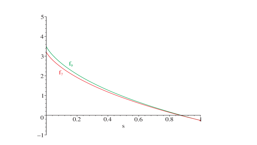
Figure 2: The functions $f_{7}(s)$ and $f_{9}(s)$.

The cancellation of IR divergences is obtained by combining $d\Gamma^{A}_{[4]}/ds$ with the ${\cal O}(\alpha_{s})$ terms in

$$\frac{d\Gamma^{A}_{[3]}}{ds}=-\kappa_{F}^{2}C_{A}s^{1-\epsilon}(1-s)^{2-2\epsilon}\Gamma(1-\epsilon)\left(\frac{m_{b}}{4\pi}\right)^{\epsilon}\left[16A_{D4}A_{D4}^{\prime}\right]~{}.$$ (4.37)

Notice that, as explicitly indicated, in this case one should use the one-loop expressions of $A$ and $A^{\prime}$ computed in the hybrid scheme, given in Eqs. (4.24). Isolating the ${\cal O}(\alpha_{s})$ terms we get

$$\!\!\!\frac{d\Gamma^{A(1)}_{[3]}}{ds}=\frac{4\alpha_{s}}{3\pi}\kappa_{F}^{2}C_{A}s^{-\epsilon}(1-s)^{2-4\epsilon}\Gamma(1+\epsilon)\Gamma(1-\epsilon)$$

$$\ \times\left\{\left[\frac{2}{\epsilon^{2}}+\frac{5}{\epsilon}+4\mbox{Li}_{2}(s)+\frac{2+4s}{s}\ln(1-s)+11\right]\mbox{Re}\left(s\widetilde{C}_{10}^{\rm eff*}\widetilde{C}_{9}^{\rm eff}\right)\right.$$

$$\quad\left.+\left[\frac{2}{\epsilon^{2}}+\frac{5}{\epsilon}+4\mbox{Li}_{2}(s)+\frac{1+5s}{s}\ln(1-s)+15+8\ln\left(\frac{\mu}{m_{b}}\right)\right]\mbox{Re}\left(2\widetilde{C}_{10}^{\rm eff*}\widetilde{C}_{7}^{\rm eff}\right)\frac{}{}\right\}\qquad$$ (4.38)

and by means of Eqs. (4.36) and (4.38) we finally obtain

$$\tau_{910}(s) = -\frac{5}{2}+\frac{1}{3(1-s)}-\frac{s(6-7s)}{3(1-s)^{2}}\ln(s)-\frac{2}{9s}(3-5s+2s^{2})\ln(1-s)+\frac{1}{3}f_{9}(s)~{},\qquad$$

$$\tau_{710}(s) = -\frac{5}{2}+\frac{1}{3(1-s)}-\frac{s(6-7s)}{3(1-s)^{2}}\ln(s)-\frac{1}{9s}(3-7s+4s^{2})\ln(1-s)+\frac{1}{3}f_{7}(s)~{}.\qquad$$ (4.39)

5 Phenomenological analysis

The results for $\sigma_{i}(s)$ and $\tau_{i}(s)$ functions, which encode bremsstrahlung and virtual IR corrections to $R(s)$ and $A_{\rm FB}(s)$, and which we have determined in the previous section, are summarized in Fig. 3. As anticipated, in all cases, except for very small values of $s$, the universal contribution of the $\sigma_{i}(s)$ is largely dominant with respect to the non-universal contribution of the $\tau_{i}$ terms. The natural scale of these corrections is $\sigma_{i}\alpha(m_{b})/\pi=O(10\%)$, and they thus represent a numerically important effect both in the rate and in the FB asymmetry.

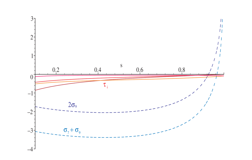
Figure 3: The functions $\sigma_{i}(s)$ (dashed lines) and $\tau_{i}(s)$ (full lines). At $s=0.1$ the $\tau_{i}(s)$ functions are ordered as follows (from top to bottom): $\tau_{910}$, $\tau_{79}$, $\tau_{710}$, and $\tau_{99}$ (almost identical to $\tau_{77}$, not explicitely shown).

A detailed phenomenological analysis of $R(s)$ and $A_{\rm FB}(s)$, including all NNLL effects, will be presented elsewhere, together with an independent calculation of the two-loop matrix-element corrections [21], which extends existing calculations also to the high-dilepton-mass region. Here we shall limit ourselves to analysing how the zero of the FB asymmetry ($s_{0}$) is modified by the inclusion of bremsstrahlung and virtual IR corrections. As is well known, this quantity, defined by $A_{\rm FB}(s_{0})=0$, is particularly interesting to determine relative sign and magnitude of the Wilson coefficients $C_{7}$ and $C_{9}$.

Employing the counting rule of Ref. [11], i.e. treating the formally $O(1/\alpha_{s})$ term of $\widetilde{C}_{9}^{\rm eff}$ as $O(1)$ (see discussion at the end of Section 3), the lowest-order value of $s_{0}$ (formally derived by the NLL expression of $A_{\rm FB}$) is determined by the solution of

$$s_{0}\widetilde{C}_{9}^{\rm eff}(s_{0})+2\widetilde{C}_{7}^{\rm eff}=0~{}.$$ (5.40)

Using the values of the effective coefficients at $\mu=5$ GeV reported in Ref. [11], this leads to

$$s^{\rm NLL}_{0}=0.14\pm 0.02~{},$$ (5.41)

where the error is determined by the scale dependence ($2.5~{}\rm{GeV}\leq\mu\leq 10$ GeV).

Neglecting the small contribution of $\delta_{\rm FB}$ [see Eq. (3.6)], the next-to-leading order equation for $s_{0}$ reads

$$s_{0}C^{\rm new}_{9}(s_{0})\left(1+\frac{\alpha_{s}}{\pi}\tau_{910}(s_{0})\right)+2C^{\rm new}_{7}(s_{0})\left(1+\frac{\alpha_{s}}{\pi}\tau_{710}(s_{0})\right)=0~{},$$ (5.42)

which leads to

$$s^{\rm NNLL}_{0}=0.162\pm 0.008~{}.$$ (5.43)

In this case the variation of the result induced by the scale dependence is accidentally very small (about $\pm 1\%$ for $2.5~{}\rm{GeV}\leq\mu\leq 10$ GeV) and we believe it cannot be used as a good estimate of higher-order corrections: taking into account the separate scale variation of both $C^{\rm new}_{9}$ and $C^{\rm new}_{7}$, and the charm-mass dependence, we estimate a conservative overall error on $s_{0}$ of about $5\%$.

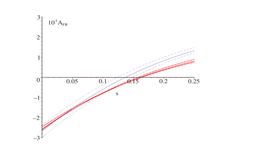
Figure 4: Comparison between NNLL and NLL results for $A_{\rm FB}(s)$ in the low $s$ region. The three thick (red) lines are the NNLL predictions for $\mu=5$ GeV (full), and $\mu=2.5$ and 10 GeV (dashed); the dotted (blue) curves are the corresponding NLL results. All curves have been obtained for $m_{c}/m_{b}=0.29$.

We recall that the new effective Wilson coefficients defined in (3.7) include not only purely UV virtual terms, but also universal bremsstrahlung and corresponding IR virtual corrections (parametrized in $\sigma_{i}$). The global effect of the bremsstrahlung and virtual IR corrections we have evaluated is that of reducing by $\sim 11\%$ the large ($\sim 27\%$) shift between $s^{\rm NNLL}_{0}$ and $s^{\rm NLL}_{0}$ induced by the NNLL UV virtual terms:

$$\left.\frac{\delta s_{0}}{s_{0}}\right|_{\sigma_{i},\tau_{i}}=\frac{\alpha_{s}}{\pi}\left[\sigma_{7}(s_{0})-\sigma_{9}(s_{0})+\tau_{710}(s_{0})-\tau_{910}(s_{0})\right]=-0.11~{}.$$ (5.44)

On the other hand, it is clear that the reduction of the error (or the reduction of the scale dependence) in Eq. (5.43) is only due to the inclusion of the UV virtual corrections computed in Ref. [11]. An illustration of the shift of the central value and the reduced scale dependence between NNL and NNLL expressions of $A_{\rm FB}(s)$, in the low $s$ region, is presented in Fig. 4. We note that in this region the nonperturbative $1/m_{b}^{2}$ and $1/m_{c}^{2}$ corrections to $A_{\rm FB}(s)$ are very small [8, 9, 10] and can safely neglected compared to the uncertainties of the partonic calculation.

Interestingly, at this level of precision, the result obtained using the ordinary LL expansion is very similar to the one obtained using the phenomenological counting rule of Ref. [11]. Indeed, at a pure NNLL level, i.e. neglecting all $O(\alpha_{s})$ terms in $C^{\rm new}_{7}$ and retaining the $O(\alpha^{-1}_{s}\times\alpha_{s})$ terms of $C^{\rm new}_{9}$, we also find as central value $s^{\rm NNLL}_{0}=0.16$.

6 Summary

The inclusive $B\rightarrow X_{s}\ell^{+}\ell^{-}$ transition, which is starting to be accessible at $B$ factories [5], represents a new source of theoretically clean observables, complementary to the $B\rightarrow X_{s}\gamma$ rate. In particular, kinematic observables such as the invariant-dilepton-mass spectrum and the lepton forward–backward asymmetry in $B\rightarrow X_{s}\ell^{+}\ell^{-}$, provide a clean information on short-distance couplings not accessible in $B\rightarrow X_{s}\gamma$.

In the present paper we calculated bremsstrahlung and corresponding virtual corrections in $B\rightarrow X_{s}\ell^{+}\ell^{-}$. We used a full dimensional regularization scheme of infrared divergences (both soft and collinear ones), which also avoids any ambiguity related to the definition of $\gamma_{5}$.

For the dilepton-invariant-mass spectrum, these contributions have already been evaluated in Refs. [11, 12], using a different technique. Our results are in complete agreement with those. We also presented the first computation of the soft-gluon (and corresponding virtual) corrections in the FB asymmetry, with the help of which we evaluated this observable systematically to NNLL precision for the first time.

The new contributions are rather important and significantly improve the sensitivity of the inclusive $B\rightarrow X_{s}l^{+}l^{-}$ decay in testing extensions of the Standard Model in the sector of flavour dynamics. In particular, the corrections we have computed shift by about 10% the position of the zero of the FB asymmetry. The complete effect of NNLL contributions to this interesting observable adds up to a $16\%$ shift compared with the NLL result, with a residual error due to higher-order terms reduced at the 5% level.

Added Note

After this work was completed, an independent calculation of NNLL corrections to the FB asymmetry appeared [26]. We find complete agreement with the results of Ref. [26] and we thank Christoph Greub for useful correspondence, which allow us to correct a typo in Eqs. (4.26) (which affected the $s\to 0$ behaviour of the plot in Fig. 2).

Appendix: Auxiliary definitions

$\bullet\,$ The function $h(z)$ describing next-to-leading order QCD corrections to the semileptonic decay [see Eq. (3.2)] is given by [22]:

$$h(z)= -(1-z^{2})\,\left(\frac{25}{4}-\frac{239}{3}\,z+\frac{25}{4}\,z^{2}\right)+z\,\ln(z)\left(20+90\,z-\frac{4}{3}\,z^{2}+\frac{17}{3}\,z^{3}\right)$$

$$+z^{2}\,\ln^{2}(z)\,(36+z^{2})+(1-z^{2})\,\left(\frac{17}{3}-\frac{64}{3}\,z+\frac{17}{3}\,z^{2}\right)\,\ln(1-z)$$

$$-4\,(1+30\,z^{2}+z^{4})\,\ln(z)\ln(1-z)-(1+16\,z^{2}+z^{4})\left(6\,\mbox{Li}(z)-\pi^{2}\right)$$

$$-32\,z^{3/2}(1+z)\left[\pi^{2}-4\,\mbox{Li}(\sqrt{z})+4\,\mbox{Li}(-\sqrt{z})-2\ln(z)\,\ln\left(\frac{1-\sqrt{z}}{1+\sqrt{z}}\right)\right]~{}.$$

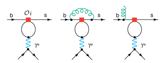
Figure A1: Examples of virtual and bremsstrahlung contributions of the four-quark operators ${\cal O}_{1\ldots 6}$ that are automatically taken into account by the redefinition of the Wilson coefficients in Eq. (A.1).

$\bullet\,$ The effective coefficients $\widetilde{C}_{7-10}^{\rm eff}$ appearing in Eq. (3.7) are defined as:

$$\widetilde{C}_{7}^{\rm eff} = \frac{4\pi}{\alpha_{s}(\mu)}C_{7}(\mu)-\frac{1}{3}C_{3}(\mu)-\frac{4}{9}C_{4}(\mu)-\frac{20}{3}C_{5}(\mu)-\frac{80}{9}C_{6}(\mu)$$

$$\widetilde{C}_{8}^{\rm eff} = \frac{4\pi}{\alpha_{s}(\mu)}C_{8}(\mu)+C_{3}(\mu)-\frac{1}{6}C_{4}(\mu)+20C_{5}(\mu)-\frac{10}{3}C_{6}(\mu)$$

$$\widetilde{C}_{9}^{\rm eff}(s) = \frac{4\pi}{\alpha_{s}(\mu)}C_{9}(\mu)+\sum_{i=1}^{6}C_{i}(\mu)\gamma^{(0)}_{i9}\ln\left(\frac{m_{b}}{\mu}\right)$$

$$+ h\left(z,s\right)\left(\frac{4}{3}C_{1}(\mu)+C_{2}(\mu)+6C_{3}(\mu)+60C_{5}(\mu)\right)$$

$$+ h(1,s)\left(-\frac{7}{2}C_{3}(\mu)-\frac{2}{3}C_{4}(\mu)-38C_{5}(\mu)-\frac{32}{3}C_{6}(\mu)\right)$$

$$+ h(0,s)\left(-\frac{1}{2}C_{3}(\mu)-\frac{2}{3}C_{4}(\mu)-8C_{5}(\mu)-\frac{32}{3}C_{6}(\mu)\right)$$

$$+ \frac{4}{3}C_{3}(\mu)+\frac{64}{9}C_{5}(\mu)+\frac{64}{27}C_{6}(\mu)$$

$$\widetilde{C}_{10}^{\rm eff} = \frac{4\pi}{\alpha_{s}(\mu)}C_{10}(\mu)~{},$$ (A.1)

where

$$h(z,s) = -\frac{4}{9}\ln(z)+\frac{8}{27}+\frac{16}{9}\frac{z}{s}-\frac{2}{9}\left(2+\frac{4\,z}{s}\right)\sqrt{\left|\frac{4\,z-s}{s}\right|}\times$$ (A.4)

$$\times \left\{\begin{array}[]{ll}2\arctan\sqrt{\frac{s}{4\,z-s}}&\mbox{for}\,s<4\,z\,,\\ \ln\left(\frac{\sqrt{s}+\sqrt{s-4\,z}}{\sqrt{s}-\sqrt{s-4\,z}}\right)-i\,\pi&\mbox{for}\,s>4\,z\,.\end{array}\right.$$

Note that specific one- and two-loop and matrix-element contributions of the four-quark operators ${\cal O}_{1-6}$ (including the corresponding bremsstrahlung contributions) such as the one shown in Fig. A1 are automatically included by the redefinition of the Wilson coefficients $C_{7}$, $C_{9}$ and $C_{10}$ given in (A.1). In fact, using this redefinition, the bremsstrahlung and virtual corrections that were shown in Fig. 1 automatically take these effects into account. The Wilson coefficients $C_{i}$ in (A.1), which are needed to NNLL precision, are given in [16].

References

- [1] G. D’Ambrosio, G.F. Giudice, G. Isidori and A. Strumia, arXiv:hep-ph/0207036.
- [2] G. Degrassi, P. Gambino and G. F. Giudice, JHEP 0012 (2000) 009 [arXiv:hep-ph/0009337]; M. Carena, D. Garcia, U. Nierste and C. E. Wagner, Phys. Lett. B 499 (2001) 141 [arXiv:hep-ph/0010003].
- [3] F. Borzumati, C. Greub, T. Hurth and D. Wyler, Phys. Rev. D 62 (2000) 075005 [arXiv:hep-ph/9911245]; T. Besmer, C. Greub and T. Hurth, Nucl. Phys. B 609 (2001) 359 [arXiv:hep-ph/0105292].
- [4] T. Hurth, in Proc. 5th Int. Symposium on Radiative Corrections (RADCOR 2000) ed. H.E. Haber, arXiv:hep-ph/0106050.
- [5] K. Senyo [BELLE Collab.], arXiv:hep-ex/0207005; K. Abe et al. [BELLE Collab.], Phys. Rev. Lett. 88 (2002) 021801 [arXiv:hep-ex/0109026]; B. Aubert et al. [BABAR Collab.], arXiv:hep-ex/0207082.
- [6] A. Ali, G. F. Giudice and T. Mannel, Z. Phys. C 67 (1995) 417 [arXiv:hep-ph/9408213]; J. L. Hewett, Phys. Rev. D 53 (1996) 4964 [arXiv:hep-ph/9506289].
- [7] A. F. Falk, M. Luke and M. J. Savage, Phys. Rev. D 49 (1994) 3367 [arXiv:hep-ph/9308288].
- [8] A. Ali, G. Hiller, L. T. Handoko and T. Morozumi, Phys. Rev. D 55 (1997) 4105 [arXiv:hep-ph/9609449].
- [9] G. Buchalla, G. Isidori and S. J. Rey, Nucl. Phys. B 511 (1998) 594 [arXiv:hep-ph/9705253].
- [10] G. Buchalla and G. Isidori, Nucl. Phys. B 525 (1998) 333 [arXiv:hep-ph/9801456].
- [11] H. H. Asatrian, H. M. Asatrian, C. Greub and M. Walker, Phys. Lett. B 507 (2001) 162 [arXiv:hep-ph/0103087]; H. H. Asatrian, H. M. Asatrian, C. Greub and M. Walker, Phys. Rev. D 65 (2002) 074004 [arXiv:hep-ph/0109140].
- [12] H. H. Asatryan, H. M. Asatrian, C. Greub and M. Walker, arXiv:hep-ph/0204341.
- [13] M. Misiak, Nucl. Phys. B 393 (1993) 23; ibid. 439 (1993) 461 (E).
- [14] A. J. Buras and M. Munz, Phys. Rev. D 52 (1995) 186 [arXiv:hep-ph/9501281].
- [15] K. Chetyrkin, M. Misiak and M. Munz, Phys. Lett. B 400 (1997) 206 [arXiv:hep-ph/9612313].
- [16] C. Bobeth, M. Misiak and J. Urban, Nucl. Phys. B 574 (2000) 291 [arXiv:hep-ph/9910220].
- [17] K. Adel and Y. Yao, Phys. Rev. D 49 (1994) 4945 [arXiv:hep-ph/9308349].
- [18] C. Greub and T. Hurth, Phys. Rev. D 56 (1997) 2934 [arXiv:hep-ph/9703349].
- [19] C. Greub, T. Hurth and D. Wyler, Phys. Lett. B 380 (1996) 385 [arXiv:hep-ph/9602281]; Phys. Rev. D 54 (1996) 3350 [arXiv:hep-ph/9603404].
- [20] A. J. Buras, A. Czarnecki, M. Misiak and J. Urban, arXiv:hep-ph/0105160.
- [21] A. Ghinculov, T. Hurth, G. Isidori and Y.-P. Yao, in preparation.
- [22] Y. Nir, Phys. Lett. B 221 (1989) 184.
- [23] P. L. Cho, M. Misiak and D. Wyler, Phys. Rev. D 54 (1996) 3329 [arXiv:hep-ph/9601360].
- [24] B. Guberina, R. D. Peccei and R. Rückl, Nucl. Phys. B 171 (1980) 333.
- [25] M. Beneke, T. Feldmann, and D. Seidel Nucl. Phys. B 612 (2001) 25.
- [26] H. M. Asatrian, K. Bieri, C. Greub and A. Hovhannisyan, arXiv:hep-ph/0209006.