DESY 02-094
hep-ph/0207300

QCD Instantons and High-Energy Diffractive Scattering

We pursue the intriguing possibility that larger-size instantons build up diffractive scattering, with the marked instanton-size scale $\langle\rho\rangle\approx 0.5$ fm being reflected in the conspicuous “geometrization” of soft QCD. As an explicit step in this direction, the known instanton-induced cross sections in deep-inelastic scattering (DIS) are transformed into the familiar colour dipole picture, which represents an intuitive framework for investigating the transition from hard to soft physics in DIS at small $x_{\rm Bj}$. The simplest instanton ($I$) process without final-state gluons is studied first. With the help of lattice results, the $q\overline{q}$-dipole size $r$ is carefully increased towards hadronic dimensions. Unlike perturbative QCD, one now observes a competition between two crucial length scales: the dipole size $r$ and the size $\rho$ of the background instanton that is sharply localized around $\langle\rho\rangle\approx 0.5$ fm. For $r\,\mbox{\,\raisebox{1.29167pt}{$>$}$\!\!\!\!\!$\raisebox{-3.87495pt}{$\sim$}}\,\,\langle\rho\rangle$, the dipole cross section indeed saturates towards a geometrical limit, proportional to the area $\pi\,\langle\rho\rangle^{2}$, subtended by the instanton. In case of final-state gluons, lattice data are crucially used to support the emerging picture and to assert the range of validity of the underlying $I\bar{I}$-valley approach. As function of an appropriate energy variable, the resulting dipole cross section turns out to be sharply peaked at the sphaleron mass in the soft regime. The general geometrical features remain like in the case without gluons.

1. QCD instantons [1] are non-perturbative fluctuations of the gluon fields, with a size distribution sharply localized around $\langle\rho\rangle\approx 0.5~{}{\rm fm}$ according to lattice simulations [2] (Fig. 1 (left)). They are well known to induce chirality-violating processes, absent in conventional perturbation theory [3]. Deep-inelastic scattering (DIS) at HERA has been shown to offer a unique opportunity [5] for discovering such processes induced by small instantons ($I$) through a sizeable rate [6, 7, 8] and a characteristic final-state signature [5, 9, 10]. An intriguing but non-conclusive excess of events in an “instanton-sensitive” data sample, has recently been reported in the first dedicated search for instanton-induced processes in DIS at HERA [11].

The validity of $I$-perturbation theory in DIS is warranted by some (generic) hard momentum scale $\mathcal{Q}$ that ensures a dynamical suppression [6] of contributions from larger size instantons with $\rho\mbox{\,\raisebox{1.29167pt}{$>$}$\!\!\!\!\!$\raisebox{-3.87495pt}{$\sim$}}\,\mathcal{O}(1/\mathcal{Q})$. Here, the above mentioned intrinsic instanton-size scale $\langle\rho\rangle\approx 0.5~{}{\rm fm}$ is correspondingly unimportant.

This paper, in contrast, is devoted to the intriguing question about the rôle of larger-size instantons and the associated intrinsic scale $\langle\rho\rangle\approx 0.5~{}{\rm fm}$, for decreasing ($Q^{2},\,x_{\rm Bj}$) towards the soft scattering regime. A number of authors have focused attention recently on the interesting possibility that larger-size instantons may well be associated with a dominant part of soft high-energy scattering, or even make up diffractive scattering altogether [12, 13, 14, 15, 16, 17]. We shall argue below that the instanton scale $\langle\rho\rangle$ is reflected in the conspicuous geometrization of soft QCD.

There are two immediate qualitative reasons for this idea. First of all, instantons represent truly non-perturbative gluons that naturally bring in an intrinsic size scale $\langle\rho\rangle\approx 0.5~{}{\rm fm}$ of hadronic dimension (Fig. 1 (left)). The instanton size happens to be surprisingly close to a corresponding “diffractive” size scale, $R_{I\!\!P}=\,R\,\sqrt{\alpha^{\prime}_{I\!\!P}/\alpha^{\prime}}\approx 0.5$ fm, resulting from simple dimensional rescaling along with a generic hadronic size $R\approx 1$ fm and the abnormally small ${I\!\!P}$omeron slope $\alpha^{\prime}_{I\!\!P}\approx\frac{1}{4}\,\alpha^{\prime}$ in terms of the normal, universal Regge slope $\alpha^{\prime}$.

Secondly, we know already from $I$-perturbation theory that the instanton contribution tends to strongly increase towards the infrared regime [5, 7, 9]. The mechanism for the decreasing instanton suppression with increasing energy is known since a long time [18, 16]: Feeding increasing energy into the scattering process makes the picture shift from one of tunneling between vacua ($E\approx 0$) to that of the actual creation of the sphaleron-like configuration [19] on top of the potential barrier of height [5] $E=M_{\rm sph}\propto\frac{1}{\alpha_{s}\rho_{\rm eff.}}$. In a second step, the action is real and the sphaleron then decays into a multi-parton final state.

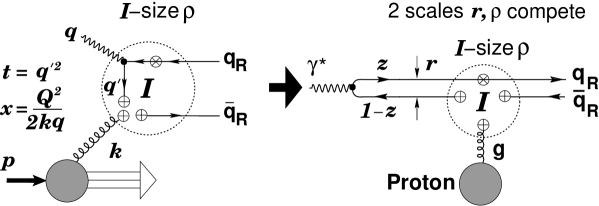
Figure 1: (Left) UKQCD lattice data [2, 8, 10] of the $(I+\bar{I})$-size distribution for quenched QCD ($n_{f}=0)$. Both the sharply defined $I$-size scale $\langle\rho\rangle\approx 0.5$ fm and the parameter-free agreement with $I$-perturbation theory [8, 10] for $\rho\mbox{\,\raisebox{1.1625pt}{$<$}$\!\!\!\!\!$\raisebox{-3.48746pt}{$\sim$}\,}0.35$ fm are apparent (solid line $\Leftrightarrow$ Eq. (8) with 3-loop expression of $\alpha_{\rm s}$ and $\Lambda^{(\rm n_{f}=0)}_{\rm\overline{MS}}=238$ MeV [22]). (Right) Transcription of the simplest $I$-induced process ($n_{f}=1,\ n_{g}=0$) with variables $x$ and $t$ into the colour dipole picture with the variables $z$ and $\mathbf{r}$

The familiar colour dipole picture [20] represents a convenient and intuitive framework for investigating the transition from hard to soft physics (diffraction) in DIS at small $x_{\rm Bj}$. At the same time, this picture is very well suited for studying the crucial interplay between the $q\overline{q}$-dipole size $r$ and the instanton size $\rho$ in an explicit and well-defined manner, as we shall discuss next.

The intuitive content of the colour dipole picture is that at high energies, in the proton’s rest frame, the virtual photon fluctuates predominantly into a $q\overline{q}$-dipole a long distance upstream of the target proton. The large difference of the $\gamma^{\ast}\rightarrow q\overline{q}$-dipole formation and $(q\overline{q})$-$P$ interaction times in the proton’s rest frame at small $x_{\rm Bj}$ then generically gives rise to the familiar factorized expression of the inclusive photon-proton cross sections,

$$\sigma_{L,T}(x_{\rm Bj},Q^{2})=\int_{0}^{1}dz\int d^{2}\mathbf{r}\;|\Psi_{L,T}(z,r)|^{2}\,\sigma_{\rm dipole}(r,\ldots),$$ (1)

in terms of the modulus squared of the (light-cone) wave function of the virtual photon, calculable in pQCD ($\hat{Q}=\sqrt{z\,(1-z)}\,Q;\ r=\mid{\mathbf{r}}\mid$),

$$\mid\Psi^{\rm pQCD}_{L\atop T}(z,r)\mid^{\,2}=\sum_{q}e_{q}^{2}\,\frac{6\alpha_{\rm em}\,\hat{Q}^{2}}{(2\pi)^{2}}\,{\rm K}_{0\atop 1}(\hat{Q}\,r)^{2}\left\{\begin{array}[]{l}4\,z\,(1-z)\\ (z^{2}+(1-z)^{2})\,,\end{array}\right.$$ (2)

and the $q\overline{q}$-dipole - nucleon cross section $\sigma_{\rm dipole}(r,\ldots)$. The variables in Eq. (1) denote the transverse $(q\overline{q})$-size $\mathbf{r}$ and the photon’s longitudinal momentum fraction $z$ carried by the quark. $\Psi_{L,T}(z,r)$ contains the dependence on the $\gamma^{\ast}$-helicity. The dipole cross section is expected to include in general the main non-perturbative contributions. For small $r$, however, one finds within pQCD [20, 21] that $\sigma_{\rm dipole}$ vanishes with the area $\pi r^{2}$ of the $q\overline{q}$-dipole. Besides this phenomenon of “colour transparency” for small $r$, the dipole cross section is expected to saturate towards a constant, once the $q\overline{q}$-separation $r$ has reached hadronic distances.

$$\sigma_{\rm dipole}\ \left\{\begin{array}[]{lrcl}\sim&\pi\,r^{\,2},&{r}^{2}\mbox{\,\raisebox{1.29167pt}{$<$}$\!\!\!\!\!$\raisebox{-3.87495pt}{$\sim$}\,}\mathcal{O}(\frac{1}{Q^{2}}),&\mbox{\rm\ ``colour transparency''~{}\cite[cite]{[\@@bibref{}{dipole,dipole-pqcd}{}{}]}},\\[4.30554pt] \approx&{\rm constant},&r\,\mbox{\,\raisebox{1.29167pt}{$>$}$\!\!\!\!\!$\raisebox{-3.87495pt}{$\sim$}}\,\,0.5{\rm\ fm},&\mbox{\rm\ ``hadron-like,\ saturation''.}\end{array}\right.$$

The strategy is now to transform the known results on $I$-induced processes in DIS into this intuitive colour dipole picture. We shall begin with the most transparent case of the simplest $I$-induced process [6],

$$\gamma^{\ast}\,g\stackrel{{\scriptstyle(I)}}{{\Rightarrow}}q_{\rm R}\ \overline{q}_{\rm R},$$ (3)

for one flavour and no final-state gluons. Subsequently, we shall turn to the more realistic case [7] with final-state gluons and $n_{f}\ (=3)$ light flavours.

The idea is to consider first large $Q^{2}$ and appropriate cuts on the variables $z$ and $r$, such that $I$-perturbation theory holds. By exploiting the lattice results on the instanton-size distribution (Fig. 1 (left)), we shall then carefully increase the $q\overline{q}$-dipole size $r$ towards hadronic dimensions.

2. Let us start by recalling the relevant results [6] for the simplest $I$-induced DIS process (3), corresponding to one flavour ($n_{f}=1$) and no final-state gluons (Fig. 1 right). At small $x_{\rm Bj}=\frac{Q^{2}}{2\,P\cdot q}$, the leading $I$-induced contribution to the respective partonic cross sections comes from the $\gamma^{\ast}g$ subprocess. In terms of the gluon density $G(x_{\rm Bj},\mu^{2})$, the results from Ref. [6] for the $\gamma^{\ast}N$ cross sections $\sigma_{T}(x_{\rm Bj},Q^{2})$ and $\sigma_{L}(x_{\rm Bj},Q^{2})$ for transverse ($T$) and longitudinal ($L$) virtual photons, respectively, then take the following form,

$$\sigma_{L,T}(x_{\rm Bj},Q^{2}) = \int_{x_{\rm Bj}}^{1}\frac{dx}{x}\left(\frac{x_{\rm Bj}}{x}\right)G\left(\frac{x_{\rm Bj}}{x},\mu^{2}\right)\int dt\,\frac{d\hat{\sigma}_{L,T}^{\gamma^{*}g}(x,t,Q^{2})}{dt};\,$$ (4)

$$\frac{d\hat{\sigma}_{L}^{\gamma^{*}g}}{dt} = \frac{\pi^{7}}{2}\frac{e_{q}^{2}}{Q^{2}}\frac{\alpha_{\rm em}}{\alpha_{\rm s}}\left[x(1-x)\sqrt{tu}\,\frac{\mathcal{R}(\sqrt{-t})-\mathcal{R}(Q)}{t+Q^{2}}-(t\leftrightarrow u)\right]^{\,2}$$ (5)

$$\frac{d\hat{\sigma}_{T}^{\gamma^{*}g}}{dt} = \frac{\pi^{7}}{8}\frac{e_{q}^{2}}{Q^{2}}\frac{\alpha_{\rm em}}{\alpha_{\rm s}}x(1-x)\left\{\left[\mathcal{R}(\sqrt{-t})^{\,2}+tu\left(\frac{\mathcal{R}(\sqrt{-t})-\mathcal{R}(Q)}{t+Q^{2}}\right)^{\,2}+(t\leftrightarrow u)\right]\right.$$ (6)

$$\left.+tu\left[\frac{\mathcal{R}(\sqrt{-t})-\mathcal{R}(Q)}{t+Q^{2}}-(t\leftrightarrow u)\right]^{\,2}(2x(1-x)-1)\right\}.$$

Eqs. (5), (6) involve the master integral $\mathcal{R}(\mathcal{Q})$ with dimensions of a length,

$$\mathcal{R}(\mathcal{Q})=\int_{0}^{\infty}d\rho\,D(\rho)\rho^{5}(\mathcal{Q}\rho)\mbox{K}_{1}(\mathcal{Q}\rho).$$ (7)

The $I$-size distribution $D(\rho)$ enters in Eq. (7) as a crucial building block of the $I$-calculus. For small $\rho$ (probed at large $\mathcal{Q}$) $D(\rho)$ is explicitly known within $I$-perturbation theory [3, 23]. Correspondingly, in Ref. [6], the integral (7) was carried out explicitly by specializing on the familiar $I$-perturbative form (renormalization scale $\mu_{r}$),

$$D(\rho)\,\Rightarrow\,D^{(I)}_{I-{\rm pert}}(\rho)=D^{(\bar{I})}_{I-{\rm pert}}(\rho) = \frac{d_{\rm\overline{MS}}}{\rho^{\,5}}\left(\frac{2\pi}{\alpha_{\rm\overline{MS}}(\mu_{r})}\right)^{6}\exp{\left(-\frac{2\pi}{\alpha_{\rm\overline{MS}}(\mu_{r})}\right)}(\rho\,\mu_{r})^{b},$$ (8)

$$b = \beta_{0}+(\beta_{1}-12\,\beta_{0})\frac{\alpha_{\rm\overline{MS}}(\mu_{r})}{4\,\pi}$$ (9)

in terms of the QCD $\beta$-function coefficients, $\beta_{0}=11-\frac{2}{3}{n_{f}},\ \beta_{1}=102-\frac{38}{3}{n_{f}}$ and the known, scheme-dependent constant $d_{\rm\overline{MS}}=C_{1}\exp[-3C_{2}+n_{f}C_{3}]/2$ with $C1=0.46628,\ C_{2}=1.51137$, and $C_{3}=0.29175$. In this form, it satisfies renormalization-group invariance at the two-loop level [23], i.e. $D^{-1}_{\,I-{\rm pert}}\,d\,D_{\,I-{\rm pert}}/d\,\ln(\mu_{r})=\mathcal{O}(\alpha_{\rm s})^{2}$.

In this paper we prefer to adopt a more general attitude concerning the form of $D(\rho)$ and thus leave the integral (7) unevaluated for the time being. For larger $I$-size $\rho$ (as relevant for smaller $\mathcal{Q}$), $D(\rho)$ is known from lattice simulations (Fig. 1 (left)). A striking feature is the strong peaking of $D_{\rm lattice}(\rho)$ around $\langle\rho\rangle\approx 0.5$ fm, whence $\mathcal{R}(0)=\int_{0}^{\infty}d\rho\;D_{\rm lattice}(\rho)\rho^{5}$ is finite. For $D_{\rm lattice}(\rho)$ from Fig. 1 (left), one finds $\mathcal{R}(0)$ to be numerically close to $\langle\rho\rangle$.

By means of an appropriate change of variables and a subsequent $2d$-Fourier transformation, Eqs. (4) - (6) may indeed be cast into a colour dipole form,

$$\sigma_{L,T}=\int_{x_{\rm Bj}}^{1}\frac{dx}{x}\int dt\,\frac{d\hat{\sigma}_{L,T}^{\gamma^{*}g}}{dt}\,\{\ldots\}\Rightarrow\int dz\int d^{2}\mathbf{r}\,\left(|\Psi_{L,T}|^{2}\sigma_{\rm dipole}\right)^{(I)}.$$ (10)

The change of variables used is $(t,\ x)\Rightarrow(\mathbf{l}^{2},z)$, with $\mathbf{l}$ being the quark transverse momentum and $z$ the photon’s longitudinal momentum fraction carried by the quark,

$$\left.\mbox{$\begin{array}[]{rclclcl}-t&=&Q^{\prime\,2}&=&\frac{\hat{Q}^{2}+l^{2}}{z};\hskip 8.61108pt-u&=&\frac{\hat{Q}^{2}+l^{2}}{1-z}\\[4.30554pt] x&&\phantom{Q^{\prime\,2}}&=&\frac{\hat{Q}^{2}}{\hat{Q}^{2}+l^{2}};\end{array}$}\right\}\hskip 8.61108pt\hat{Q}=\sqrt{z\,(1-z)}\,Q;\hskip 12.91663ptl=\mid\mathbf{l}\mid.$$ (11)

The subsequent $2d$-Fourier transformation then introduces the transverse $q\overline{q}$ distance $\mathbf{r}$ of the colour-dipole picture via

$$G(r,\ldots) = \int\frac{d^{2}\mathbf{l}}{(2\,\pi)^{2}}\,e^{i\mathbf{r}\cdot\mathbf{l}}\,\tilde{G}(l,\ldots)=\frac{1}{2\,\pi}\,\int dl\,l\,{\rm J}_{0}(l\,r)\,\tilde{G}(l,\ldots);\hskip 8.61108pt\mbox{\rm\ and}$$ (12)

$$\int\frac{d^{2}\mathbf{l}}{(2\pi)^{2}}\,\tilde{G}(l,\ldots)^{2} = \int d^{2}\mathbf{r}\,G(r,\ldots)^{2};\hskip 4.30554pt\int\frac{d^{2}\mathbf{l}}{(2\,\pi)^{2}}\,l^{2}\,\tilde{G}(l,\ldots)^{2}=\int d^{2}\mathbf{r}\,\left(\frac{d}{dr}G(r,\ldots)\right)^{2}.$$ (13)

Like is usual in pQCD-calculations [21], we throughout invoke the familiar “leading-$\log(1/x_{\rm Bj})$” - approximation, $x_{\rm Bj}/x\,G(x_{\rm Bj}/x,\mu^{2})\approx x_{\rm Bj}G(x_{\rm Bj},\mu^{2})$, for simplicity. In terms of the familiar pQCD wave function (2) of the photon, we then obtain from Eqs. (4) - (6) the following integrands on the r.h.s. of Eqs. (10),

$$\left(\left|\Psi_{L}\right|^{2}\sigma_{\rm dipole}\right)^{(I)}\approx\,\mid\Psi_{L}^{\rm pQCD}(z,r)\mid^{\,2}\,\frac{1}{\alpha_{\rm s}}\,x_{\rm Bj}\,G(x_{\rm Bj},\mu^{2})\,\frac{\pi^{8}}{12}$$ (14)

$$\times\left\{\int_{0}^{\infty}\,d\rho\,D(\rho)\,\rho^{5}\,\left(\frac{-\frac{d}{dr^{2}}\left(2r^{2}\frac{\mbox{K}_{1}(\hat{Q}\sqrt{r^{2}+\rho^{2}/z})}{\hat{Q}\sqrt{r^{2}+\rho^{2}/z}}\right)}{{\rm K}_{0}(\hat{Q}r)}-(z\leftrightarrow 1-z)\right)\right\}^{2},$$

$$\left(\left|\Psi_{T}\right|^{2}\sigma_{\rm dipole}\right)^{(I)}\approx\,\mid\Psi_{T}^{\rm pQCD}(z,r)\mid^{\,2}\,\frac{1}{\alpha_{\rm s}}\,x_{\rm Bj}\,G(x_{\rm Bj},\mu^{2})\,\frac{\pi^{8}}{12}$$ (15)

$$\times\left\{\left(\int_{0}^{\infty}\,d\rho\,D(\rho)\,\rho^{5}\,\frac{\frac{r\,\mbox{K}_{1}(\hat{Q}\sqrt{r^{2}+\rho^{2}/z})}{\sqrt{r^{2}+\rho^{2}/z}}}{{\rm K}_{1}(\hat{Q}r)\sqrt{z^{2}+(1-z)^{2}}}\right)^{\,2}+(z\leftrightarrow 1-z)+\ldots\right\}.$$

As expected, one explicitly observes a competition between two crucial length scales in Eqs. (14), (15): the size $r$ of the $q\overline{q}$-dipole and the typical size of the background instanton of about $\langle\rho\rangle\approx 0.5~{}{\rm fm}$. Like in pQCD, the asymmetric configuration, $z\gg 1-z$ or $1-z\gg z$, obviously dominates.

The validity of strict $I$-perturbation theory ($D(\rho)\equiv D_{I-{\rm pert}}(\rho)$ in Eq. (7)) requires the presence of a hard scale $\mathcal{Q}$ along with certain cuts. However, after replacing $D(\rho)$ by $D_{\rm lattice}(\rho)$ (Fig. 1 (left)), these restrictions are at least no longer necessary for reasons of convergence of the $\rho$-integral (7) etc., and one may tentatively increase the dipole size $r$ towards hadronic dimensions.

Next, we note in Eqs. (14), (15),

$$-\frac{d}{d\,r^{2}}\left(2\,r^{2}\frac{{\rm K}_{1}\left(\hat{Q}\sqrt{r^{2}+\rho^{2}/z}\right)}{\hat{Q}\sqrt{r^{2}+\rho^{2}/z}}\right) \approx \left\{\begin{array}[]{rl}-\frac{{\rm K}_{1}\left(Q\,\rho\sqrt{1-z}\right)}{Q\,\rho\sqrt{1-z}}&\frac{r^{2}\,z}{\rho^{2}}\Rightarrow 0,\\[8.61108pt] {\rm K}_{0}\left(\hat{Q}\,r\right)&\frac{r^{2}\,z}{\rho^{2}}\mbox{\ large}.\end{array}\right.$$ (18)

$$r\frac{{\rm K}_{1}\left(\hat{Q}\sqrt{r^{2}+\rho^{2}/z}\right)}{\sqrt{r^{2}+\rho^{2}/z}} \approx \left\{\begin{array}[]{rl}\phantom{-\frac{{\rm K}_{1}\left(Q\,\rho\sqrt{1-z}\right)}{Q\,\rho\sqrt{1-z}}}&\phantom{\frac{r^{2}\,z}{\rho^{2}}\Rightarrow 0,}\vspace{-3ex}\\ \mathcal{O}(\frac{r\sqrt{z}}{\rho})&\frac{r^{2}\,z}{\rho^{2}}\Rightarrow 0,\\[8.61108pt] {\rm K}_{1}\left(\hat{Q}\,r\right)&\frac{r^{2}\,z}{\rho^{2}}\mbox{\ large}.\end{array}\right.$$ (22)

Due to the strong peaking of $D_{\rm lattice}(\rho)$ around $\rho\approx\langle\rho\rangle$, one finds from Eqs. (14) - (22) for the limiting cases of interest ($z\gg 1-z$ without restriction),

$$\begin{array}[]{|c|c|}\hline\cr r&\rule[-5.69054pt]{0.0pt}{25.60747pt}\left(\mid\Psi_{L,T}\mid^{\,2}\sigma_{\rm dipole}\right)^{(I)}\\[4.30554pt] \hline\cr\rule[5.69054pt]{0.0pt}{11.38109pt}\Rightarrow 0&\mathcal{O}(1),\mbox{\rm\ but\ exponentially\ small\ for\ large}\ \hat{Q},\\[12.91663pt] &\rule[-5.69054pt]{0.0pt}{19.91692pt}\mid\Psi^{\rm\,pQCD}_{L,T}\mid^{\,2}\,\sigma_{\rm dipole}^{(I)}\hskip 8.61108pt\mbox{\rm\ with}\\ \raisebox{10.76385pt}[-6.45831pt]{$\mbox{\,\raisebox{1.29167pt}{$>$}$\!\!\!\!\!$\raisebox{-3.87495pt}{$\sim$}}\,\langle\rho\rangle$}&\displaystyle\rule[-8.53581pt]{0.0pt}{31.29802pt}\sigma^{(I)}_{\rm dipole}(r,\ldots)=\frac{1}{\alpha_{\rm s}}\,x_{\rm Bj}\,G(x_{\rm Bj},\mu^{2})\,\frac{\pi^{8}}{12}\,\left(\int_{0}^{\infty}\,d\rho\,D_{\rm lattice}(\rho)\,\rho^{5}\right)^{2}.\\[12.91663pt] \hline\cr\end{array}$$ (23)

In summary: As apparent in Eqs. (14), (15), (23), the dipole cross section from the simplest $I$-induced process raises strongly around the instanton scale, $r\approx\langle\rho\rangle$, and indeed saturates for large $r/\langle\rho\rangle$ towards a constant geometrical limit, proportional to the area $\pi\,\mathcal{R}(0)^{2}\,=\,\pi\left(\int_{0}^{\infty}\,d\rho\,D_{\rm lattice}(\rho)\,\rho^{5}\right)^{2}$, subtended by the instanton. Clearly, without the crucial information about $D(\rho)$ from the lattice (Fig. 1 (left)), the result would be infinite. Note the inverse power of $\alpha_{\rm s}$ in front of $\sigma_{\rm dipole}^{(I)}$ in Eq. (23), signalling its non-perturbative nature.

3. We are now ready to turn to the more realistic $I$-induced inclusive process

$$\gamma^{\ast}+g\stackrel{{\scriptstyle(I)}}{{\Rightarrow}}n_{f}\,(q_{\rm R}+\overline{q}_{\rm R})+\mbox{\rm\ gluons}.$$ (24)

The corresponding DIS cross sections have been previously worked out in detail [7] and are implemented in the Monte-Carlo generator QCDINS [9] that forms a basic tool in experimental searches for $I$-induced events at HERA [11].

The differential cross sections entering in Eqs. (4) now take a modified form [7] $(Q^{\prime\,2}=-t)$,

$$\frac{d\hat{\sigma}_{L,\,\Sigma}^{\gamma^{\ast}g}}{d\,Q^{\prime\,2}} = \frac{8\pi^{2}\alpha_{\rm em}}{Q^{2}}\,\sum_{q}\,e_{q}^{2}\,\int\frac{d{x^{\prime}}}{{x^{\prime}}}\,\frac{x}{{x^{\prime}}}\,P_{L,\,\Sigma}\left(x,{x^{\prime}},\frac{Q^{\prime 2}}{Q^{2}}\right)\,\sigma^{(I)}_{q^{\ast}g}({x^{\prime}},Q^{\prime\,2}),$$ (25)

$$\frac{d\sigma_{T}^{\gamma^{\ast}g}}{d\,Q^{\prime\,2}} = \frac{1}{2}\,\left(\frac{d\sigma_{\Sigma}^{\gamma^{\ast}g}}{d\,Q^{\prime\,2}}+\frac{d\sigma_{L}^{\gamma^{\ast}g}}{d\,Q^{\prime\,2}}\right).$$ (26)

The $\gamma^{\ast}\Rightarrow\overline{q}\,q$ “flux” factors [7, 28],

$$P_{{\rm L}\atop{\rm\Sigma}}\left(x,{x^{\prime}},\frac{Q^{\prime 2}}{Q^{2}}\right)=\frac{3}{16\pi^{3}}\frac{x}{{x^{\prime}}}\left\{\begin{array}[]{l}2\,\frac{x}{x^{\prime}}\,\frac{Q^{\prime 2}}{Q^{2}}\,\left(1-\frac{Q^{\prime 2}}{Q^{2}}\frac{x}{{x^{\prime}}}\right)\,\frac{1-{x^{\prime}}}{{x^{\prime}}}\\[6.45831pt] \left(1+\frac{1}{x}-\frac{1}{{x^{\prime}}}-\frac{Q^{\prime 2}}{Q^{2}}\right)\end{array}\right.,$$ (29)

turn out to be directly related to the square of the pQCD photon wave function, $\mid\Psi^{\rm pQCD}_{L,\,T}\mid^{2}$ as we shall see explicitly below. Corresponding to the more complex final state, Eqs. (25), (26) now involve an additional integration over the Bjorken-$x^{\prime}$ variable $1\geq x^{\prime}\equiv Q^{\,\prime\,2}/(2p\cdot q^{\prime})\geq x\geq 0$ of the $I$-induced subprocess,

$$\left\{\overline{q}^{\,\ast}\mbox{\rm\ or\ }q^{\,\ast}\right\}\ (q^{\prime})+g\ (p)\stackrel{{\scriptstyle(I)}}{{\Rightarrow}}X,$$ (30)

with total cross section $\sigma^{(I)}_{q^{\ast}g}({x^{\prime}},Q^{\prime\,2})$ that includes the main instanton dynamics (see below).

By means of a change of variables like in Eqs. (11), except for the replacement $x\Rightarrow x/x^{\prime}$ due to $x^{\prime}\neq 1$, one now finds approximately (assuming $z\gg(1-z)$ throughout without restriction),

$$\sigma_{L,\,T}(x_{\rm Bj},Q^{2}) \approx \int dz\int\frac{d^{2}\mathbf{l}}{(2\pi)^{2}}\mid\tilde{\Psi}^{\rm pQCD}_{L,\,T}(z,l)\mid^{2}\,\tilde{\sigma}^{(I)}_{\rm dipole}(l,x_{\rm Bj},\ldots);\hskip 12.91663pt\mbox{\rm with}$$ (31)

$$\mid\tilde{\Psi}^{\rm pQCD}_{L\atop T}(z,l)\mid^{2} = \sum_{q}e_{q}^{2}\frac{6\alpha_{\rm em}\,\hat{Q}^{2}}{(\hat{Q}^{2}+l^{2})^{2}}\left\{\begin{array}[]{l}4\,z\,(1-z)\\ l^{2}/\hat{Q}^{2}\,(z^{2}+(1-z)^{2})\end{array}\right.$$ (34)

$$\tilde{\sigma}^{(I)}_{\rm dipole}(l,x_{\rm Bj},\ldots) \approx x_{\rm Bj}\,G(x_{\rm Bj},\mu^{2})\,\int_{0}^{\sqrt{s^{\,\prime}_{\rm max}}}d\,E\left[\frac{\left((p+q^{\prime})^{2}\right)^{3/2}}{4\,(p\cdot q^{\prime})\,Q^{\,\prime 2}}\,\sigma^{(I)}_{q^{\ast}\,g}\left(E,\frac{\hat{Q}^{2}+l^{2}}{z}\right)\right].$$ (35)

Since the total c.m. energy $\sqrt{s^{\,\prime}}$ of the $q^{\ast}\,g\Rightarrow X$ subprocess (30) is given by $\sqrt{s^{\,\prime}}=Q^{\prime}\,\sqrt{1/x^{\prime}-1}$, the $x^{\prime}$ integration above is equivalent to an integration over $E\equiv\sqrt{s^{\,\prime}}$. The function $\tilde{\Psi}^{\rm pQCD}_{L,\,T}(z,l)$ is just the $2d$-Fourier transform (cf. Eq. (12)) of $\Psi^{\rm pQCD}_{L,\,T}(z,r)$ in Eq. (2). By inserting the known results for $\sigma^{(I)}_{q^{\ast}g}$ from Ref. [7] into Eq. (35), one finds the following structure for $\tilde{\sigma}^{(I)}_{\rm dipole}(l,x_{\rm Bj},\ldots)$,

$$\frac{d\tilde{\sigma}^{(I)}_{\rm dipole}}{dE} \approx \frac{1}{\alpha_{\rm s}}\,x_{\rm Bj}\,G(x_{\rm Bj},\mu^{2})\,\frac{\pi^{5}}{6}\,\int_{0}^{\infty}d\,\rho\,D(\rho)\,\rho^{5}\,(\rho\,Q^{\prime}){\rm K_{1}}(\rho\,Q^{\prime})\int_{0}^{\infty}d\,\bar{\rho}\,D(\bar{\rho})\,\bar{\rho}^{5}\,(\bar{\rho}\,Q^{\prime}){\rm K_{1}}(\bar{\rho}\,Q^{\prime})\,$$ (36)

$$\times\int\frac{d^{4}R}{(\rho\bar{\rho})^{3/2}}\,e^{i\,(p+q^{\prime})\cdot R}\,\int dU\,e^{-\frac{4\pi}{\alpha_{\rm s}}\,\Omega_{\rm valley}\left(\xi\left(\frac{R^{2}}{\rho\bar{\rho}},\frac{\rho}{\bar{\rho}}\right),U\right)}\left\{\ldots\right\};\hskip 12.91663pt\sqrt{(p+q^{\prime})^{2}}=E.$$

For reasons of space, we have skipped in $\{\ldots\}$ some (flavour dependent) prefactors of secondary importance. The second line in Eq. (36) is largely associated with the final-state gluons. Let us briefly recall some of the essential features.

While in case of the simplest $I$-induced process (3) above, the contribution to the total cross section was obtained by explicitly squaring the scattering amplitude and integrating over the final-state phase space, the derivation of the DIS results [7] for the inclusive process (24) was based on the optical theorem combined with the $I\bar{I}$-valley method [24]. In this approach [25, 26, 7], one most efficiently evaluates the total cross section from the imaginary part of the forward elastic amplitude induced by the $I\bar{I}$-valley background $A_{\mu}^{(I\bar{I})}$. This method elegantly accounts for a resummation and exponentiation of the final-state gluons, whose effects are encoded in the explicitly known $I\bar{I}$-valley interaction [26, 27],

$$\Omega_{\rm valley}(\xi,U)=S^{(I\bar{I})}_{\rm valley}(\xi,U)-1=\frac{\alpha_{\rm s}}{4\pi}\,S[A_{\mu}^{(I\bar{I})}]-1,$$ (37)

appearing in Eq. (36). Apart from its dependence on the relative $I\bar{I}$-orientation $U$ in colour space, the valley action is restricted by conformal invariance to depend only on the dimensionless, “conformal separation”

$$\xi\equiv\frac{-R^{2}+i\epsilon R_{0}}{\rho\bar{\rho}}+\frac{\rho}{\bar{\rho}}+\frac{\bar{\rho}}{\rho},$$ (38)

where in Euclidean space, the collective coordinate $R^{(E)}_{\mu}$ denotes the $I\bar{I}$-distance 4-vector, with $-R^{2}\Rightarrow R^{2\,(E)}\geq 0$ such that $\xi^{(E)}\geq 2$.

In principle, the next step is to transform Eq. (36) further into the $(\mathbf{r},z)$ colour-dipole representation, in generalization of Eq. (23). To this end, however, we first have to locate any possible, additional $l^{2}=l^{2}(Q^{\,\prime\,2},x/x^{\prime},Q^{2})$ dependences that might arise from the final-state gluons etc., i.e. from the second line in Eq. (36). Let us begin by exhibiting a number of important features of $d\tilde{\sigma}^{(I)}_{\rm dipole}/dE$ in Eq. (36) that emerge in the softer $Q^{\,\prime}$ regime in combination with lattice results.

Besides the $I$-size distribution $D(\rho)$, the $I\bar{I}$-interaction $\Omega$ in Eq. (36) represents a second crucial quantity of the $I$-calculus, for which we shall exploit independent lattice information that will be instrumental for a transition towards softer $Q^{\prime}$. Fig. 2 (left) displays (normalized) UKQCD lattice data [2, 8, 10] of the $I\bar{I}$-distance distribution versus the (Euclidean) $I\bar{I}$-distance $R\equiv\sqrt{R^{\,2\,(E)}}$ in units of $\langle\rho\rangle$ for quenched QCD ($n_{f}=0$), along with the prediction of the $I\bar{I}$-valley approach [8],

$$\frac{dn^{\rm valley}_{I\bar{I}}}{d^{4}\,x\,d^{4}\,R}=\int_{0}^{\infty}d\rho\,D_{\rm lattice}(\rho)\,\int_{0}^{\infty}d\bar{\rho}\,D_{\rm lattice}(\bar{\rho})\,\int d\,U\,e^{-\frac{4\pi}{\alpha_{\rm s}(s/\sqrt{\rho\bar{\rho}})}\,\Omega_{\rm valley}\left(\xi\left(\frac{R^{2}}{\rho\bar{\rho}},\frac{\rho}{\bar{\rho}}\right),U\right)}.$$ (39)

Note the remarkable similarity in structure of this lattice “observable” and $d\tilde{\sigma}^{(I)}_{\rm dipole}/dE$ in Eq. (36). This holds notably in the soft $Q^{\prime}$ regime where the exponential suppression of larger size instantons via the ${\rm K}_{1}$ Bessel functions in Eq. (36) tends to vanish, i. e. $(\rho Q^{\prime})\,{\rm K}_{1}(\rho Q^{\prime})\sim 1$, and instead $\rho\approx\bar{\rho}\approx\rho_{\rm peak}\approx\langle\rho\rangle$, with $\rho_{\rm peak}$ and $\langle\rho\rangle$ being the (close-by) positions of the sharp peaks of $\rho^{5}\,D_{\rm lattice}(\rho)$ and $D_{\rm lattice}(\rho)$, respectively (cf. Fig. 1 (left)).

Figure 2: (Left) UKQCD lattice data [2, 8, 10] of the (normalized) $I\bar{I}$-distance distribution versus the $I\bar{I}$-distance $R$ in units of $\langle\rho\rangle$ for quenched QCD ($n_{f}=0$). The $I\bar{I}$-valley approximation appears to be reliable down to $R/\langle\rho\rangle\approx 1$, where it breaks down abruptly. (Middle) If $\rho\approx\rho_{\rm peak}$, as is the case in Eq. (36) towards soft $Q^{\prime}$, the saddle-point relation (42) associates $E/M_{\rm sph}=1$ with $R^{\ast}/\rho=1$. The weak s-dependence signals approximate renormalization group invariance ($\mu_{r}=s/\rho$ ). (Right) The $I\bar{I}$-distance distribution, being largely a measure of $\left\langle\exp{\left[-\frac{4\pi}{\alpha_{\rm s}(s/\rho_{\rm peak})}\,\Omega_{\rm valley}(\xi,U)\right]}\right\rangle_{U}$ in Eq. (36), displayed versus energy in units of the QCD sphaleron mass $M_{\rm sph}$. While the valley prediction continues to rise for $E/M_{\rm sph}>1$, the lattice data provide the first direct evidence that the $I\bar{I}$-valley approach is adequate right up to $E\approx M_{\rm sph}$, where the dominant contribution to the scattering process arises.

Indeed, Fig. 2 (left) reveals crucial information concerning the range of validity of the $I\bar{I}$-valley interaction $\Omega_{\rm valley}$. The $I\bar{I}$-valley approximation appears to be quite reliable down to $\left(\frac{R}{\langle\rho\rangle}\right)_{\rm min}\approx 1$, where the $I\bar{I}$-distribution shows a sharp peak, while the valley prediction continues to rise indefinitely. According to Eq. (38), with $\rho\approx\bar{\rho}$, this peak of the lattice data corresponds to $\xi_{\rm peak}\approx 3$ and hence to $S^{(I\bar{I})}_{\rm valley}(\xi_{\rm peak}=3,U^{\ast})\approx\frac{1}{2}$, for the most attractive $I\bar{I}$ colour orientation $U=U^{\ast}$ that is known to dominate the U-integral in Eqs. (36) at least for sufficiently large values of $4\pi/\alpha_{\rm s}$ in form of a saddle point. This important result perfectly matches with previous theoretical claims [29, 30], according to which the maximal $I$-induced (QCD or EW) cross section shows a “square-root” enhancement compared to the pure tunneling behaviour at $E=0$ ($S^{(I\bar{I})}_{\rm valley}(\xi=\infty,U^{\ast})=1$).

Let us demonstrate next that this marked peak of the lattice $I\bar{I}$-distance distribution in Fig. 2 (left) in fact corresponds to the top of the potential barrier, i. e. to the sphaleron mass, $E\approx M_{\rm sph}$, which may be estimated [30] as the potential energy of the instanton field exactly in the middle of the transition when the instanton passes the $N_{\rm Chern-Simons}=1/2$ point,

$$M_{\rm sph}(\rho)=\frac{1}{g_{\rm s}^{2}}\,\frac{1}{4}\,4\pi\,\int dr\,r^{2}\,\frac{96\rho^{4}}{(t^{2}+r^{2}+\rho^{2})^{4}}_{\mid t=0}=\frac{3\pi}{4}\,\frac{1}{\alpha_{\rm s}\,\rho}.$$ (40)

This result for $M_{\rm sph}$ matches with the estimate $M_{\rm sph}\sim Q^{\,\prime}$ from Ref. [5] at large $Q^{\,\prime}$, where the integrals in Eq. (36) are known to be dominated by a unique saddle-point in all integration variables, notably including $\rho=\bar{\rho}\approx\rho^{\ast}(Q^{\,\prime})\sim 1/(\alpha_{\rm s}\,Q^{\,\prime})$.

For large $Q^{\prime}$, the familiar saddle point [7],

$$\rho^{\ast}=\bar{\rho}^{\,\ast}\sim\frac{1}{\alpha_{\rm s}\,Q^{\,\prime}};\hskip 8.61108ptR^{\,\ast}_{\mu}=(-i\rho^{\ast}\sqrt{\xi^{\ast}(x^{\prime})-2},\ \mathbf{0}),$$ (41)

of the effective exponent $\Gamma$ in Eq. (36) is determined by requiring $\Gamma$ to be stationary with respect to all integration variables. In particular, the combination of $\partial\Gamma/\partial\xi=0$ and $\partial\Gamma/\partial\rho=0$ leads to a unique solution $\xi^{\ast}=\xi^{\ast}(x^{\prime},\ldots)$ for all physical values of $x^{\prime}$, $x\leq x^{\prime}\leq 1$.

However, the situation changes drastically, in the softer $Q^{\prime}$-regime, where $\rho\approx\rho_{\rm peak}\approx 0.59$ fm with $\rho_{\rm peak}$ corresponding to the sharp peak position of $\rho^{5}\,D_{\rm lattice}(\rho)$ in Eq. (36). Here, effectively only $\partial\Gamma/\partial\xi=0$ remains and provides together with Eq. (40), a correlation of $E/M_{\rm sph}(\rho)$ and $\xi^{\ast}=2+R^{\,2\,(E)\,\ast}/\rho^{\,2}$ for $\rho\Rightarrow\rho_{\rm peak}$. At 2-loop renormalization group accuracy, we obtain from Eq. (17) of Ref. [7], with renormalization scale $\mu=s/\rho$ and $s=\mathcal{O}(1)$ (e. g. $s_{I}\approx 1.18$, cf. Ref. [8]),

$$\frac{E}{M_{\rm sph}}={\frac{32}{3}}\,\frac{d\,\Omega_{\rm valley}(\xi^{\ast})}{d\xi}\,\sqrt{{\xi^{\ast}}-2}\,\left(1-\frac{1}{2\,\pi}\,\ln(s)\,\alpha_{\rm s}\left({\frac{s}{{\rho}}}\right){\beta_{0}}-\frac{1}{8\,\pi^{2}}\,\ln(s)\,\alpha_{\rm s}\left({\frac{s}{{\rho}}}\right)^{2}{\beta_{1}}\right).$$ (42)

First of all, we notice from Eq. (42) that for soft $Q^{\prime}$, a saddle-point solution for $\xi^{\ast}$ only exists if $E/M_{\rm sph}$ is not too large. The reason is that $\frac{32}{3}\,\frac{d\,\Omega_{\rm valley}(\xi^{\ast})}{d\xi}\sqrt{{\xi^{\ast}}-2}\,\mbox{\,\raisebox{1.29167pt}{$<$}$\!\!\!\!\!$\raisebox{-3.87495pt}{$\sim$}\,}\,3.5$, with the maximum attained around $\xi^{\ast}\approx 2.4$, i. e. quite near to the striking peak position $\xi_{\rm peak}\approx 3$ of the lattice data for the $I\bar{I}$-distance distribution above. Hence, it is tempting to ask, for which values of $\rho$ and the scheme parameter $s$ the peak value $\xi_{\rm peak}=3$ would exactly correspond to $E=M_{\rm sph}$. The solution from Eq. (42) with a 3-loop expression for $\alpha_{\rm s}$ and $\Lambda^{(\rm nf=0)}_{\rm\overline{MS}}=238$ MeV from the lattice [22] is displayed in Figs. 2 (middle), (right) and nicely confirms our intuitive expectations.

In summary: For soft $Q^{\,\prime}$, i. e. $\rho\approx\rho_{\rm peak}$ and increasing total energy E of the $I$-subprocess (30), $0\mbox{\,\raisebox{1.29167pt}{$<$}$\!\!\!\!\!$\raisebox{-3.87495pt}{$\sim$}\,}E<M_{\rm sph}(\rho_{\rm peak})$, the (Euclidean) saddle-point solution $\xi^{\ast}$ of Eq. (42) decreases such that $d\tilde{\sigma}^{(I)}_{\rm dipole}/dE$ in Eq. (36) steeply increases until a sharp maximum is reached. Fig. 2 (right) illustrates this behaviour by displaying instead the $I\bar{I}$-distance distribution that is largely a measure of $\left\langle\exp{\left[-\frac{4\pi}{\alpha_{\rm s}(s/\rho_{\rm peak})}\,\Omega_{\rm valley}(\xi,U)\right]}\right\rangle_{U}$, versus $E/M_{\rm sph}$ from Eq. (42). Fig. 2 (middle) shows that the maximum position $R\approx\rho_{\rm peak}$, as inferred from lattice data, indeed corresponds to the top of the potential barrier, i.e. to $E\approx M_{\rm sph}$, provided $Q^{\,\prime}$ approaches the soft regime and thus stirs $\rho,\bar{\rho}$ towards $\rho_{\rm peak}$ in Eq. (36). For $E>M_{\rm sph}$ the Euclidean saddle point $R_{0}=-i\rho^{\ast}\sqrt{\xi(E/M_{\rm sph})-2}$, described by Eq. (42), ceases to exist and $d\tilde{\sigma}^{(I)}_{\rm dipole}/dE$ may be estimated from the peaking of $\left\langle\exp{\left[-\frac{4\pi}{\alpha_{\rm s}(s/\rho_{\rm peak})}\,\Omega_{\rm valley}(\xi,U)\right]}\right\rangle_{U}$ (lattice) to decrease again in this regime. Finally, from the lattice data, the underlying $I\bar{I}$-valley approximation has been found to interpolate reliably between the pure tunneling regime ($E=0$) and the sphaleron at the top of the potential barrier ($E=M_{\rm sph}$). Altogether, the resulting picture is in qualitative agreement with the findings of Refs. [29, 14].

In view of the above analysis, the integration over the total $I$-subprocess energy $E$ in Eqs. (35), (36) up to $E=\sqrt{s^{\,\prime}_{\rm max}}$, may evidently be extended to $E\Rightarrow\infty$ due to the strong peaking of $d\tilde{\sigma}^{(I)}_{\rm dipole}/dE$ around $E\approx M_{\rm sph}(\rho_{\rm peak})<\sqrt{s^{\,\prime}_{\rm max}}$,

$$\tilde{\sigma}^{(I)}_{\rm dipole}(l,\ldots)\approx\int_{0}^{\infty}dE\;\frac{d\tilde{\sigma}^{(I)}_{\rm dipole}}{dE}\approx\frac{1}{\alpha_{\rm s}}\,x_{\rm Bj}\,G(x_{\rm Bj},\mu^{2})\,\frac{\pi^{5}}{6}$$ (43)

$$\times\int_{0}^{\infty}d\rho\,D(\rho)\,\rho^{5}\,(\rho\,Q^{\prime}){\rm K_{1}}(\rho\,Q^{\prime})\int_{0}^{\infty}d\bar{\rho}\,D(\bar{\rho})\,\bar{\rho}^{5}\,(\bar{\rho}\,Q^{\prime}){\rm K_{1}}(\bar{\rho}\,Q^{\prime})\,H_{\rm sph}(\rho,\bar{\rho}),$$

with the dimensionless function $H_{\rm sph}(\rho,\bar{\rho})$, being largely associated with the final-state gluons,

$$H_{\rm sph}(\rho,\bar{\rho})\approx\int_{0}^{\infty}dE\,\int\frac{d^{4}R}{(\rho\bar{\rho})^{3/2}}\,e^{i\,(p+q^{\prime})\cdot R}\int d\,U\;e^{-\frac{4\pi}{\alpha_{\rm s}(s/\sqrt{\rho\bar{\rho}})}\,\Omega_{\rm lattice}\left(\xi\left(\frac{R^{2}}{\rho\bar{\rho}},\frac{\rho}{\bar{\rho}}\right),U\right)}\left\{\ldots\right\}.$$ (44)

In the soft $Q^{\prime}$ regime, $H_{\rm sph}(\rho,\bar{\rho})$ does not introduce any additional $l$-dependences beyond those coming from the “master integrals” $\mathcal{R}\left((\hat{Q}^{2}+l^{2})/z\right)$ in Eq. (43) in analogy to Eq. (7) in case of the simplest $I$-induced process. Hence we may perform the $2d$-Fourier transformation $(\mathbf{l}\Rightarrow\mathbf{r})$ and finally obtain (for $z\gg(1-z)$ without restriction) e. g.,

$$\left(\left|\Psi_{L}\right|^{2}\sigma_{\rm dipole}\right)^{(I)}\approx\,\mid\Psi_{L}^{\rm pQCD}(z,r)\mid^{\,2}\,\frac{1}{\alpha_{\rm s}}\,x_{\rm Bj}\,G(x_{\rm Bj},\mu^{2})\,\frac{\pi^{5}}{6}$$ (45)

$$\times\int_{0}^{\infty}\,d\rho\,D(\rho)\,\rho^{5}\,\int_{0}^{\infty}\,d\bar{\rho}\,D(\bar{\rho})\,\bar{\rho}^{\,5}\,H_{\rm sph}(\rho,\bar{\rho})\,\frac{-\frac{d}{dr^{2}}\left(2r^{2}\frac{\mbox{K}_{1}(\hat{Q}\sqrt{r^{2}+\rho^{2}/z})}{\hat{Q}\sqrt{r^{2}+\rho^{2}/z}}\right)\times(\rho\leftrightarrow\bar{\rho})}{{\rm K}_{0}(\hat{Q}r)^{2}}.$$

For $r\mbox{\,\raisebox{1.29167pt}{$>$}$\!\!\!\!\!$\raisebox{-3.87495pt}{$\sim$}}\,\langle\rho\rangle$,

$$\left(\left|\Psi_{L}\right|^{2}\sigma_{\rm dipole}\right)^{(I)}\approx\,\mid\Psi_{L}^{\rm pQCD}(z,r)\mid^{\,2}\,\sigma_{\rm dipole}^{(I)\,{\rm gluons}},$$ (46)

with

$$\sigma_{\rm dipole}^{(I)\,{\rm gluons}}=\frac{1}{\alpha_{\rm s}}\,x_{\rm Bj}\,G(x_{\rm Bj},\mu^{2})\,\frac{\pi^{5}}{6}\left(\int_{0}^{\infty}\,d\rho\,D_{\rm lattice}(\rho)\,\rho^{5}\right)^{2}H_{\rm sph}(\langle\rho\rangle,\langle\rho\rangle).$$ (47)

Similar to the simplest $I$-induced process (23), the result exhibits a saturating, geometrical limit, proportional to the area $\pi\,\mathcal{R}(0)^{2}=\pi\left(\int_{0}^{\infty}\,d\rho\,D_{\rm lattice}(\rho)\,\rho^{5}\right)^{2}$, subtended by the instanton.

Outlook: An investigation of the phenomenology associated with the emerging picture of soft high-energy processes induced by instantons is challenging and in progress [31]. Before more quantitative predictions can be made, a careful study of inherent uncertainties are necessary. Let us merely state at this point that the instanton-induced contributions indeed appear significant towards the soft regime. Like in case of the extensively studied DIS processes (HERA) induced by small instantons (cf. e. g. Refs. [15, 11]), one expects characteristic final-state signatures. Given the importance of lattice data for the conclusions reached in this paper, further improved lattice results in this direction would be most desirable. While the main intention of this paper was to associate the origin of the conspicuous geometrical scale in diffractive scattering with the average instanton size, clearly, a number of important aspects remain to be investigated. For instance, an understanding of the mechanism that causes the cross section to increase with energy in an instanton framework is of importance.

Acknowledgements: We are grateful to Leonid Frankfurt and Mark Strikman for valuable discussions and thank Andreas Ringwald for a careful reading of the manuscript.

References

• [1] A. Belavin et al., Phys. Lett. B 59 (1975) 85.
• [2] D.A. Smith and M.J. Teper (UKQCD), Phys. Rev. D 58 (1998) 014505.
• [3] G. ‘t Hooft, Phys. Rev. Lett. 37 (1976) 8; Phys. Rev. D 14 (1976) 3432; Phys. Rev. D 18 (1978) 2199 (Erratum); Phys. Rep. 142 (1986) 357.
• [4] I. Balitsky and V. Braun, Phys. Lett. B 314 (1993) 237.
• [5] A. Ringwald and F. Schrempp, Proc. Quarks ’94, ed D.Yu. Grigoriev et al. (Singapore: World Scientific) p 170, [arXiv:hep-ph/9411217].
• [6] S. Moch, A. Ringwald and F. Schrempp, Nucl. Phys. B 507 (1997) 134.
• [7] A. Ringwald and F. Schrempp, Phys. Lett. B 438 (1998) 217.
• [8] A. Ringwald and F. Schrempp, Phys. Lett. B 459 (1999) 249.
• [9] A. Ringwald and F. Schrempp, Comput. Phys. Commun. 132 (2000) 267.
• [10] A. Ringwald and F. Schrempp, Phys. Lett. B 503 (2001) 331.
• [11] C. Adloff et al. [H1 Collaboration], arXiv:hep-ex/0205078.
• [12] D.E. Kharzeev, Y.V. Kovchegov and E. Levin, Nucl. Phys. A 690 (2001) 621.
• [13] E. Shuryak and I. Zahed, Phys. Rev. D 62 (2000) 085014.
• [14] M. A. Nowak, E. V. Shuryak and I. Zahed, Phys. Rev. D 64 (2001) 034008.
• [15] F. Schrempp, J. Phys. G 28 (2002) 915, [arXiv:hep-ph/0109032].
• [16] D.M. Ostrovsky, G.W. Carter and E.V. Shuryak, arXiv:hep-ph/0204224.
• [17] F. Schrempp and A. Utermann, arXiv:hep-ph/0207052, to be published in Proc. 10th Int. Workshop on Deep Inelastic Scattering (DIS2002), Cracow, Poland, 2002.
• [18] H. Aoyama and H. Goldberg, Phys. Lett. B 188 (1987) 506; A. Ringwald, Nucl. Phys. B 330 (1990) 1; O. Espinosa, Nucl. Phys. B 343 (1990) 310.
• [19] F. R. Klinkhamer and N. S. Manton, Phys. Rev. D 30 (1984) 2212.
• [20] N. Nikolaev and B.G. Zakharov, Z. Phys. C 49 (1990) 607; Z. Phys. C 53 (1992) 331; A.H. Mueller, Nucl. Phys. B 415 (1994) 373.
• [21] F. E. Low, Phys. Rev. D 12 (1975) 163; L. Frankfurt, G.A. Miller and M. Strikman, Phys. Lett. B 304 (1993) 1.
• [22] S. Capitani, M. Lüscher, R. Sommer and H. Wittig, Nucl. Phys. B 544 (1999) 669.
• [23] T. Morris, D. Ross and C. Sachrajda, Nucl. Phys. B 255 (1985) 115.
• [24] A. Yung, Nucl. Phys. B 297 (1988) 47.
• [25] M. Porrati, Nucl. Phys. B 347 (1990) 371; V.V. Khoze and A. Ringwald, Nucl. Phys. B 355 (1991) 351; V. Zakharov, Nucl. Phys. B 371 (1992) 637; I. Balitsky and V. Braun, Nucl. Phys. B 380 (1992) 51.
• [26] V.V. Khoze and A. Ringwald, Phys. Lett. B 259 (1991) 106.
• [27] J. Verbaarschot, Nucl. Phys. B 362 (1991) 33.
• [28] S. Moch, A. Ringwald and F. Schrempp, unpublished; S. Moch, PhD thesis, DESY T-97-02 (1997) Internal Report (unpublished).
• [29] V. Zakharov, Nucl. Phys. B 353 (1991) 683; M. Maggiore and M. Shifman, Nucl. Phys. B 365 (1991) 161; G. Veneziano, Mod. Phys. Lett. A7 (1992) 1661.
• [30] D. Diakonov and V. Petrov, Phys. Rev. D 50 (1994) 266.
• [31] F. Schrempp and A. Utermann, in preparation.