Unintegrated gluon distributions in a photon from the CCFM equation in the single loop approximation
Agnieszka Gawron and Jan Kwieciński

H. Niewodniczański Institute of Nuclear Physics, Kraków, Poland

()

The system of CCFM equations for unintegrated parton distributions in a photon is considered in the single loop approximation. We include quarks and non-singular parts of the splitting functions in the corresponding evolution equations. We solve the system of CCFM equations utilising the transverse coordinate representation which diagonalises these equations in the single loop approximation. The results for the unintegrated gluon distributions in a photon are presented and confronted with the approximate form expressing those distributions in terms of the integrated gluon and quark distributions and a suitably defined Sudakov-like form factor.

1 Introduction

Inclusive quantities describing the hard processes are controlled in the QCD improved parton model by the scale dependent quark and gluon distributions which depend upon the longitudinal momentum fraction $x$ and upon the hard scale $Q^{2}$. In order to describe less inclusive quantities which are sensitive to the transverse momentum of the parton it is however necessary to consider the distributions unintegrated over the transverse momentum of the parton [1]-[8]. Those unintegrated distributions are described in perturbative QCD by the Ciafaloni-Catani-Fiorani- Marchesini (CCFM) equation [9],[10] based upon quantum coherence which implies angular ordering [11]. It embodies in a unified way the (LO) DGLAP evolution and BFKL dynamics at low $x$.

Existing analyses of the CCFM equation concern predominantly parton distributions in a nucleon [8], [12] - [20]. The purpose of this paper is to extend this analysis to the case of the unintegrated parton distributions in a photon. We limit ourselves to the so called ’single loop’ approximation in which the CCFM equation is equivalent to the LO DGLAP evolution [12, 13]. We shall utilise the fact that in this approximation the CCFM equation is diagonalised by the Fourier-Bessel transform and so one can explore the transverse coordinate representation of this equation [21]. The transverse coordinate representation conjugate to the transverse momentum of the parton has proved to be very useful in studying $p_{t}$ distributions within the DGLAP framework and it has been widely explored in the analysis of the soft gluon resummation effects in $e^{+}e^{-}$ collisions [22],[23], in the $p_{t}$ distribution of Drell-Yan pairs [24] etc. The formalism of transverse coordinate representation adopted in our analysis of the CCFM equation is similar to that used in those studies.

The single-loop approximation of the CCFM equation which we shall use neglects important small $x$ effects and so it may not be reliable at (very) small $x$. It should however become an adequate approximation at moderately small values of $x$ (i.e. $x>0.01$ or so) which is relevant phenomenologically e.g. for the description of the heavy quark production in $\gamma\gamma$ collisions at presently available energies [25].

The CCFM equation is usually considered only for the gluonic sector and, in principle, with only the singular parts of the $g\rightarrow gg$ splitting functions included in the evolution. In order to have a formalism which is phenomenologically relevant at large and moderately small values of $x$ one has to incorporate also the quark distributions and the complete splitting functions. This is straigtforward in the ’single loop’ approximation which, after integration over the transverse momentum of the partons, should reduce the CCFM equations to the conventional DGLAP evolution equations.

The content of our paper is as follows: In the next Section we introduce the system of CCFM equations in the single loop approximation for the unintegrated parton distributions in a photon. In Section 3 we discuss the transverse coordinate representation which partially diagonalises the system of CCFM equations. In Section 4 we present results of the numerical solution of the CCFM equation(s) for the unintegrated gluon distributions in a photon. We do also discuss approximate treatment of these equations which allows to relate the unintegrated gluon distributions in a photon to the integrated gluon and quark distributions and the suitably defined Sudakov-like form-factor. Finally, in Section 5, we summarise our main results and give our conclusions.

2 The CCFM equation in the single loop approximation for the parton distributions in a photon

In this Section we introduce the system of CCFM equations for the unintegrated parton distributions in a photon. We extend the CCFM framework by including the quark distributions and the non-singular parts of the splitting functions. We limit ourselves to the single-loop approximation which should be adequate in the region of moderately small values of $x$.

The original Catani, Ciafaloni, Fiorani, Marchesini (CCFM) equation [9] for the unintegrated, scale dependent gluon distribution $f_{g}(x,Q_{t},Q)$ which is generated by the sum of ladder diagrams with angular ordering along the chain has the following form:

$$f_{g}(x,Q_{t},Q)=\tilde{f}_{g}^{0}(x,Q_{t},Q)+\int{d^{2}\mbox{\boldmath${q}$}\over\pi q^{2}}\int_{x}^{1}{dz\over z}\Theta(Q-qz)\Theta(q-q_{0}){\alpha_{s}\over 2\pi}\Delta_{s}(Q,q,z)\times$$

$$\times\left[2N_{c}\Delta_{NS}(Q_{t},q,z)+{2N_{c}z\over(1-z)}f\left({x\over z},|\mbox{\boldmath${Q}$}_{t}+(1-z)\mbox{\boldmath${q}$}|,q\right)\right],$$ (1)

where $\Delta_{S}(Q,q,z)$ and $\Delta_{NS}(Q_{t},q,z)$ are the Sudakov and non-Sudakov form factors. They are given by the following expressions:

$$\Delta_{S}(Q,q,z)=exp\left[-\int_{(qz)^{2}}^{Q^{2}}{dp^{2}\over p^{2}}{\alpha_{s}\over 2\pi}\int_{0}^{1-q_{0}/p}dzzP_{gg}(z)\right],$$ (2)

$$\Delta_{NS}(Q_{t},q,z)=exp\left[-\int_{z}^{1}{dz^{\prime}\over z^{\prime}}\int_{(qz^{\prime})^{2}}^{Q_{t}^{2}}{dp^{2}\over p^{2}}{2N_{c}\alpha_{s}\over 2\pi}\right].$$ (3)

The variables $x,Q_{t},Q$ denote the longitudinal momentum fraction, transverse momentum of the gluon and the hard scale respectively. The latter is defined in terms of the maximal emission angle [8, 9]. The constraint $\Theta(Q-qz)$ in equation (1) reflects the angular ordering and the inhomogeneous term $\tilde{f}^{0}(x,Q_{t},Q)$ is related to the input non-perturbative gluon distribution. It also contains effects of both the Sudakov and non-Sudakov form-factors [15].

In order to make the CCFM formalism realistic in the region of large and moderately small values of $x$ we should introduce, besides the unintegrated gluon distribution $f_{g}(x,Q_{t},Q)$ also the unintegrated quark distributions $f_{q_{i}}(x,Q_{t},Q)$, where $i$ numerates the quark flavour, and include the $q\rightarrow gq$, ($\bar{q}\rightarrow g\bar{q}$) and $g\rightarrow\bar{q}q$ transitions along the chain. In order to get exact correspondence with the complete LO DGLAP evolution one should also use complete splitting functions and not only their singular components. In the region of large and moderately small values of $x$ one can introduce the ’single loop’ approximation which corresponds to the replacement of the angular ordering constraint $\Theta(Q-qz)$ by $\Theta(Q-q)$ and to setting the non-Sudakov form-factor $\Delta_{NS}$ equal to unity [12, 13].

It is convenient to consider the unintegrated singlet $S$ and non-singlet ($NS$) quark distributions:

$$f_{S}(x,Q_{t},Q)=2\Sigma_{i=1}^{f}f_{q_{i}}(x,,Q_{t},Q),$$ (4)

$$f_{NS}(x,Q_{t},Q)=2\Sigma_{i=1}^{f}e_{i}^{2}f_{q_{i}}(x,,Q_{t},Q)-<e^{2}>f_{S}(x,Q_{t},Q),$$ (5)

where

$$<e^{k}>={1\over f}\Sigma_{i=1}^{f}e_{i}^{k},$$ (6)

with $e_{i}$ denoting the charge of the quark of the flavour $i$ and $f$ being equal to the number of active flavours.

It is also convenient to ’unfold’ the Sudakov form-factor(s) so that the virtual corrections and real emission terms appear on equal footing in the kernels of the corresponding system of integral equations. The unfolded system of CCFM equations in the single loop approximation takes the following form:

$$f_{NS}(x,Q_{t},Q)={\alpha_{em}\over 2\pi}{k_{NS}^{0}(x)\over Q_{t}^{2}}+f^{0}_{NS}(x,Q_{t})+$$

$$+\int_{0}^{1}dz\int{d^{2}q\over\pi q^{2}}{\alpha_{s}(q^{2})\over 2\pi}\Theta(q^{2}-q_{0}^{2})\Theta(Q-q)P_{qq}(z)\times$$

$$\times\left[\Theta(z-x)f_{NS}\left({x\over z},Q^{\prime}_{t},q\right)-f_{NS}(x,Q_{t},q)\right],$$ (7)

$$f_{S}(x,Q_{t},Q)={\alpha_{em}\over 2\pi}{k_{S}^{0}(x)\over Q_{t}^{2}}+f_{S}^{0}(x,Q_{t})+$$

$$+\int_{0}^{1}dz\int{d^{2}q\over\pi q^{2}}{\alpha_{s}(q^{2})\over 2\pi}\Theta(q^{2}-q_{0}^{2})\Theta(Q-q)\times$$

$$\times\bigg{\{}\Theta(z-x)\left[P_{qq}(z)f_{S}\left({x\over z},Q^{\prime}_{t},q\right)+P_{qg}(z)f_{g}\left({x\over z},Q^{\prime}_{t},q\right)\right]-\bigg{.}$$

$$\bigg{.}-P_{qq}(z)f_{S}(x,Q_{t},q)\bigg{\}},$$ (8)

$$f_{g}(x,Q_{t},Q)=f_{g}^{0}(x,Q_{t})+$$

$$+\int_{0}^{1}dz\int{d^{2}q\over\pi q^{2}}{\alpha_{s}(q^{2})\over 2\pi}\Theta(q^{2}-q_{0}^{2})\Theta(Q-q)\times$$

$$\times\bigg{\{}\Theta(z-x)\left[P_{gq}(z)f_{S}\left({x\over z},Q^{\prime}_{t},q\right)+P_{gg}(z)f_{g}\left({x\over z},Q^{\prime}_{t},q\right)\right]-\bigg{.}$$

$$\bigg{.}-\big{[}zP_{gg}(z)+zP_{qg}(z)\big{]}f_{g}(x,Q_{t},q)\bigg{\}},$$ (9)

where

$${\bf Q^{\prime}_{t}}={\bf Q_{t}}+(1-z){\bf q}.$$ (10)

The functions $k_{NS}^{0}(x)$ and $k_{S}^{0}(x)$ are defined as below:

$$k_{NS}^{0}(x)=2N_{c}f(<e^{4}>-<e^{2}>^{2})[x^{2}+(1-x)^{2}],$$ (11)

$$k_{S}^{0}(x)=2N_{c}f<e^{2}>[x^{2}+(1-x)^{2}],$$ (12)

with $N_{c}$ denoting the number of colours. The inhomogeneous terms proportional to $k_{NS}^{0}(x)$ and $k_{S}^{0}(x)$ in equations (7) and (8) respectively reflect the point coupling of the photon to quarks and antiquarks. The functions $f_{NS}^{0}(x,Q_{t}),f_{S}^{0}(x,Q_{t}),f_{g}^{0}(x,Q_{t})$ denote the non-perturbative ’hadronic’ components of the unintegrated non-singlet, singlet and gluon distributions respectively. The parameter $q_{0}$ is the infrared cut-off. The splitting functions $P_{ab}(z)$ are the LO splitting functions, i.e.:

$$P_{qq}(z)={4\over 3}{1+z^{2}\over 1-z},$$

$$P_{qg}(z)=f[z^{2}+(1-z)^{2}],$$

$$P_{gq}(z)={4\over 3}{1+(1-z)^{2}\over z},$$

$$P_{gg}(z)=2N_{c}\left[{z\over 1-z}+{1-z\over z}+z(1-z)\right].$$ (13)

3 CCFM equation in the transverse coordinate reprecentation

It can easily be observed that the system of CCFM equations in the single loop approximation (7) - (9) can be diagonalised by the Fourier-Bessel transform [21]:

$$f_{k}(x,Q_{t},Q)=\int_{0}^{\infty}dbbJ_{0}(Q_{t}b)\bar{f}_{k}(x,b,Q),$$ (14)

$$\bar{f}_{k}(x,b,Q)=\int_{0}^{\infty}dQ_{t}Q_{t}J_{0}(Q_{t}b)f_{k}(x,Q_{t},Q),$$ (15)

where $k=NS,S,g$ and $J_{0}(u)$ is the Bessel function. The corresponding system of CCFM equations for $\bar{f}_{NS}(x,b,Q),\bar{f}_{S}(x,b,Q)$ and $\bar{f}_{g}(x,b,Q)$ which follows from equations (7) - (9) reads:

$$\bar{f}_{NS}(x,b,Q)={\alpha_{em}\over 2\pi}k_{NS}^{0}(x)\bar{f}_{pt}^{0}(b,Q)+\bar{f}^{0}_{NS}(x,b)+$$

$$+\int_{0}^{1}dz\int{dq^{2}\over q^{2}}{\alpha_{s}(q^{2})\over 2\pi}\Theta(q^{2}-q_{0}^{2})\Theta(Q-q)P_{qq}(z)\times$$

$$\times\left[\Theta(z-x)J_{0}\big{[}(1-z)qb\big{]}\bar{f}_{NS}\left({x\over z},b,q\right)-\bar{f}_{NS}(x,b,q)\right],$$ (16)

$$f_{S}(x,Q_{t},Q)={\alpha_{em}\over 2\pi}k_{S}^{0}(x)\bar{f}_{pt}^{0}(b,Q)+\bar{f}_{S}^{0}(x,b)+$$

$$+\int_{0}^{1}dz\int{dq^{2}\over q^{2}}{\alpha_{s}(q^{2})\over 2\pi}\Theta(q^{2}-q_{0}^{2})\Theta(Q-q)\times$$

$$\times\bigg{\{}\Theta(z-x)J_{0}\big{[}(1-z)qb\big{]}\left[P_{qq}(z)\bar{f}_{S}\left({x\over z},b,q\right)+P_{qg}(z)\bar{f}_{g}\left({x\over z},b,q\right)\right]-\bigg{.}$$

$$\bigg{.}-P_{qq}(z)\bar{f}_{S}(x,b,q)\bigg{\}},$$ (17)

$$\bar{f}_{g}(x,Q_{t},Q)=\bar{f}_{g}^{0}(x,b)+$$

$$+\int_{0}^{1}dz\int{dq^{2}\over q^{2}}{\alpha_{s}(q^{2})\over 2\pi}\Theta(q^{2}-q_{0}^{2})\Theta(Q-q)\times$$

$$\times\bigg{\{}\Theta(z-x)J_{0}\big{[}(1-z)qb\big{]}\left[P_{gq}(z)\bar{f}_{S}\left({x\over z},b,q\right)+P_{gg}(z)\bar{f}_{g}\left({x\over z},b,q\right)\right]-\bigg{.}$$

$$\bigg{.}-\big{[}zP_{gg}(z)+zP_{qg}(z)\big{]}\bar{f}_{g}(x,b,q)\bigg{\}}.$$ (18)

The function $\bar{f}_{pt}^{0}(b,Q)$ controlling the inhomogeneous term originating from the point-like interaction is defined as:

$$\bar{f}_{pt}^{0}(b,Q)=\int_{q_{0}}^{Q}dQ_{t}Q_{t}{J_{0}(bQ_{t})\over Q_{t}^{2}}.$$ (19)

In the definition of the inhomogeneous term corresponding to the point interaction of the photon we have introduced upper limit cut-off equal to $Q$ in the integration over $dQ_{t}$ in equation (19). This is necessary for making the CCFM formalism compatible with the DGLAP evolution for the integrated parton distributions $f^{int}_{i}(x,Q^{2})$

$$xf^{int}_{i}(x,Q^{2})=\int_{0}^{\infty}dQ_{t}^{2}f_{i}(x,Q_{t},Q).$$ (20)

The integrated distributions $f^{int}_{i}(x,Q^{2})$ are given by the distributions $\bar{f}_{i}(x,b,Q)$ at $b=0$ i.e.

$$xf^{int}_{i}(x,Q^{2})=2\bar{f}_{i}(x,b=0,Q).$$ (21)

Equations (16) - (18) are equivalent to the following system of inhomogeneous differential equations:

$$Q^{2}{\partial\bar{f}_{NS}(x,b,Q)\over\partial Q^{2}}={\alpha_{em}\over 2\pi}k_{NS}^{0}(x){J_{0}(bQ)\over 2}+{\alpha_{s}(Q^{2})\over 2\pi}\int_{0}^{1}dzP_{qq}(z)\times$$

$$\times\left[\Theta(z-x)J_{0}\big{[}(1-z)Qb\big{]}\bar{f}_{NS}\left({x\over z},b,Q\right)-\bar{f}_{NS}(x,b,Q)\right],$$ (22)

$$Q^{2}{\partial f_{S}(x,Q_{t},Q)\over\partial Q^{2}}={\alpha_{em}\over 2\pi}k_{S}^{0}(x){J_{0}(bQ)\over 2}+{\alpha_{s}(Q^{2})\over 2\pi}\int_{0}^{1}dz\bigg{\{}\Theta(z-x)J_{0}\big{[}(1-z)Qb\big{]}\times\bigg{.}$$

$$\bigg{.}\times\left[P_{qq}(z)\bar{f}_{S}\left({x\over z},b,Q\right)+P_{qg}(z)\bar{f}_{g}\left({x\over z},b,Q\right)\right]-P_{qq}(z)\bar{f}_{S}(x,b,Q)\bigg{\}}$$ (23)

$$Q^{2}{\partial\bar{f}_{g}(x,Q_{t},Q)\over\partial Q^{2}}={\alpha_{s}(Q^{2})\over 2\pi}\int_{0}^{1}dz\bigg{\{}\Theta(z-x)J_{0}\big{[}(1-z)Qb\big{]}\times\bigg{.}$$

$$\bigg{.}\times\left[P_{gq}(z)\bar{f}_{S}\left({x\over z},b,Q\right)+P_{gg}(z)\bar{f}_{g}\left({x\over z},b,Q\right)\right]-\big{[}zP_{gg}(z)+zP_{qg}(z)\big{]}\bar{f}_{g}(x,b,Q)\bigg{\}},$$ (24)

with the initial conditions:

$$\bar{f}_{i}(x,b,q_{0})=\bar{f}_{i}^{0}(x,b),$$ (25)

where $i$ corresponds to $NS$, $S$ and $g$. In complete analogy to the integrated parton distributions in a photon we can introduce conventional decomposition of the distributions $\bar{f}_{i}(x,b,Q)$ into their point-like $\bar{f}_{i}^{p}(x,b,Q)$ and hadronic $\bar{f}_{i}^{h}(x,b,Q)$ components i.e.

$$\bar{f}_{i}(x,b,Q)=\bar{f}_{i}^{p}(x,b,Q)+\bar{f}_{i}^{h}(x,b,Q).$$ (26)

The point-like components $\bar{f}_{i}^{p}(x,b,Q)$ are the solutions of inhomogeneous equations (22) - (24) with the initial conditions

$$\bar{f}_{i}(x,b,q_{0})=0.$$ (27)

The hadronic components $\bar{f}_{i}^{h}(x,b,Q)$ are the solutions of the homogeneous equations corresponding to equations (22) - (24) with inhomogeneous terms set equal to zero. The initial conditions for the hadronic components are given by equation (25).

4 Numerical results

In this section we present results of the numerical analysis of the CCFM equation in the single loop approximation for the gluon distribution in a proton. To this aim we solved equations (23) and (24) following the LO DGLAP analysis performed at [26]. The unintegrated gluon distributions are then calculated from equation (14). We have assumed the following initial conditions for the distributions $f_{S}(x,b,Q)$ and $f_{g}(x,b,Q)$ at $Q=q_{0}$, where $q_{0}^{2}=0.26GeV^{2}$ :

$$f_{S}(x,b,q_{0})={1\over 2}x\Sigma(x,q_{0}^{2})F(b),$$ (28)

$$f_{g}(x,b,q_{0})={1\over 2}xg(x,q_{0}^{2})F(b),$$ (29)

where the form-factor $F(b)$ was assumed to have the the following form

$$F(b)=exp\left(-{b^{2}\over b_{0}^{2}}\right),$$ (30)

with $b_{0}^{2}=4GeV^{-2}$. The functions $\Sigma(x,q_{0}^{2})$ and $g(x,q_{0}^{2})$, which are the integrated singlet and gluon distributions in the photon at the reference scale were taken from refs. [26] and [27]. To be precise the parton distributions in a photon at the reference scale $Q=q_{0}$ were obtained in [26] from the VMD model with the parton distributions in vector mesons assumed to be given by those in a pion and taken from [27]. The singlet and gluon distributions in the photon at $Q^{2}=q_{0}^{2}$ are expressed in the following way in terms of the corresponding distributions in the pion:

$$x\Sigma(x,q_{0}^{2})=\alpha_{em}(G_{\rho}^{2}+G_{\omega}^{2})\big{[}xq_{v}^{\pi}(x,q_{0}^{2})+4x\bar{q}^{\pi}(x,q_{0}^{2})\big{]},$$ (31)

$$xg(x,q_{0}^{2})=\alpha_{em}(G_{\rho}^{2}+G_{\omega}^{2})xg^{\pi}(x,q_{0}^{2}),$$ (32)

with $G_{\rho}^{2}=0.5$ and $G_{\omega}^{2}=0.043$. The valence quark, antiquark and gluon distributions in a pion for $Q^{2}=q_{0}^{2}$ were parametrised as below [27]:

$$xq_{v}^{\pi}(x,q_{0}^{2})=1.129(1.+0.153\sqrt{x})x^{0.504}(1-x)^{0.349},$$ (33)

$$x\bar{q}^{\pi}(x,q_{0}^{2})=0.522(1.-3.243\sqrt{x}+5.206x)x^{0.16}(1-x)^{5.2},$$ (34)

$$xg^{\pi}(x,q_{0}^{2})=7.326(1-1.919\sqrt{x}+1.524x)x^{1.433}(1-x)^{1.326}.$$ (35)

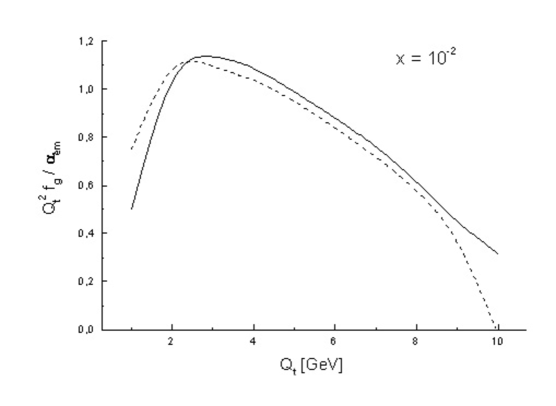
Figure 1: The function $Q_{t}^{2}f_{g}(x,Q_{t},Q)/\alpha_{em}$, where $f_{g}(x,Q_{t},Q)$ is the unintegrated gluon distribution in a photon plotted as the function of the transverse momentum $Q_{t}$ of the gluon for $x=0.01$ and $Q=10GeV$. The solid and dashed lines correspond to the exact solution of the system of the CCFM equations in the single loop approximation and to the approximate expression (36) respectively.

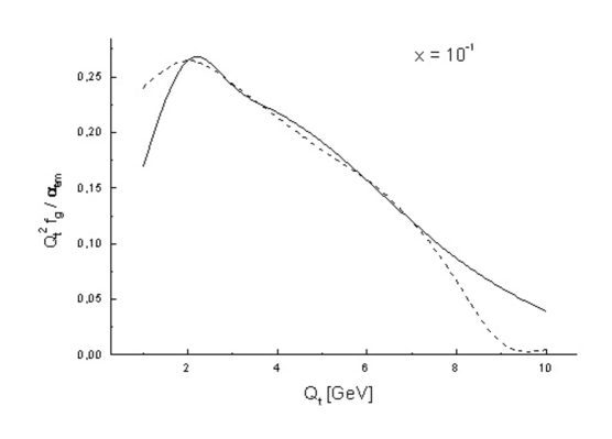
Figure 2: The function $Q_{t}^{2}f_{g}(x,Q_{t},Q)/\alpha_{em}$, where $f_{g}(x,Q_{t},Q)$ is the unintegrated gluon distribution in a photon plotted as the function of the transverse momentum $Q_{t}$ of the gluon for $x=0.1$ and $Q=10GeV$. The solid and dashed lines correspond to the exact solution of the system of the CCFM equations in the single loop approximation and to the approximate expression (36) respectively.

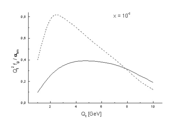
Figure 3: The point-like (solid line) and hadronic (dashed line) components of the unintegrated gluon distribution in a photon plotted as functions of the transverse momentum $Q_{t}$ of the gluon for $x=0.01$ and $Q=10GeV$.

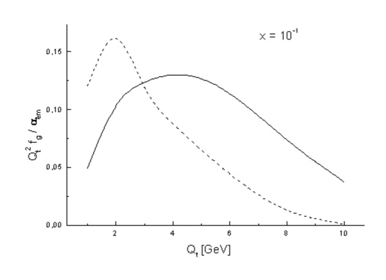
Figure 4: The point-like (solid line) and hadronic (dashed line) components of the unintegrated gluon distribution in a photon plotted as functions of the transverse momentum $Q_{t}$ of the gluon for $x=0.1$ and $Q=10GeV$.

Results of our calculations concerning unintegrated gluon distributions in the photon are presented in Figures 1 and 2. We plot in these figures $Q_{t}^{2}f_{g}(x,Q_{t},Q)/\alpha_{em}$ as the function of $Q_{t}$ at $Q=10GeV$ for two values of $x$, i.e. for $x=0.01$ (Fig. 1) and $x=0.1$ (Fig. 2). We compare our result with the approximate expression for $Q_{t}^{2}f_{g}(x,Q_{t},Q)/\alpha_{em}$:

$$Q_{t}^{2}f_{g}(x,Q_{t},Q)\simeq$$

$$\simeq{\alpha_{s}(Q_{t}^{2})T_{g}(Q_{t},Q)\over 2\pi\alpha_{em}}\int_{x}^{1-Q_{t}/Q}dz\left[P_{gg}(z){x\over z}g\left({x\over z},Q_{t}^{2}\right)+P_{gq}(z){x\over z}\Sigma\left({x\over z},Q_{t}^{2}\right)\right],$$ (36)

where the Sudakov-like form-factor is given by:

$$T_{g}(Q_{t},Q)=$$

$$exp\left\{-\int_{Q_{t}^{2}}^{Q^{2}}{dq^{2}\over q^{2}}{\alpha_{s}(q^{2})\over 2\pi}\int_{0}^{1-Q_{t}/q}dz^{\prime}\big{[}z^{\prime}P_{gg}(z^{\prime})+z^{\prime}P_{qg}(z^{\prime})\big{]}\right\}.$$ (37)

Derivation of approximate relation (36), which is similar to that discussed in [2] is given in the Appendix. We see that the approximate expression (36) reproduces reasonably well exact solution of the CCFM equation for unintegrated gluon distributions in a photon. In Figures 3 and 4 we show decomposition of the unintegrated gluon distrtibutions into their hadronic and point-like components. The point-like component is found to become increasingly important in the region of large $Q_{t}$. The relative contribution of this component does also increase with increasing $x$.

5 Summary and conclusions

We have considered in this paper the system of CCFM equations in the single loop approximation for the unintegrated parton distributions in a photon. We have extended the conventional CCFM formalism by including quarks and the complete splitting functions. We have utilised the fact that the CCFM equation(s) in the single loop approximation can be diagonalised by the Fourrier-Bessel transform. We have found that the unintegrated gluon distributions in a photon obtained from the exact solution of the system of CCFM equations in the single loop approximation can be well represented by the approximate expressions connecting the those diatributions with the integrated (gluon and quark) distributions and the Sudakov-like form-factor.

The novel feature of the CCFM equation for the parton distributions in a photon, when compared with the hadronic case is the presence of the point-like components. Those components become increasingly important at large values of $x$. They have also been found to play important role at large values of the trasnverse momentum $Q_{t}$ of the gluon for moderately small values of $x$.

The unintegrated gluon distributions which describe the $x$ and $Q_{t}$ distributions are important quantities are neede in the description of the processes which are sensitive to the transverse momentum of the gluon. Their knowledge is in particular necessary for the description of heavy quark production in $\gamma$ $\gamma$ collisions within the $k_{t}$ factorisation. Results obtained in our paper may therefore be used for the theoretical analysis of this process.

Appendix

Let us make the following approximation:

$$J(u)\simeq\Theta(1-u).$$ (38)

It is clear that in this approximation solution of equations (17,18) is independent of $b$ for $Q<1/b$, provided we neglect the $b$ dependence of the ’hadronic’ input that is justified at small $b$. ¿From (15,38) we also get:

$$f_{k}(x,Q_{t},Q)\simeq 2\quad{\partial\bar{f}_{k}(x,b=1/Q_{t},Q)\over\partial Q_{t}^{2}}.$$ (39)

It is useful to rearrange equations (17,18) as below:

$$\bar{f}_{S}(x,b,Q)={\alpha_{em}\over 2\pi}k_{S}^{0}(x)\bar{f}_{pt}^{0}(b,Q)+\bar{f}_{S}^{0}(x,b)+$$

$$+\int_{0}^{1}dz\int{dq^{2}\over q^{2}}{\alpha_{s}(q^{2})\over 2\pi}\Theta(q^{2}-q_{0}^{2})\Theta(Q-q)\times$$

$$\times\bigg{\{}J_{0}\big{[}(1-z)qb\big{]}\Big{[}\Theta(z-x)\left(P_{qq}(z)\bar{f}_{S}\left({x\over z},b,q\right)+P_{qg}(z)\bar{f}_{g}\left({x\over z},b,q\right)\right)-\Big{.}\bigg{.}$$

$$\bigg{.}\Big{.}-P_{qq}(z)\bar{f}_{S}(x,b,q)\Big{]}+P_{qq}(z)\big{(}1-J_{0}[(1-z)qb]\big{)}\bar{f}_{S}(x,b,q)\bigg{\}},$$ (40)

$$\bar{f}_{g}(x,b,Q)=\bar{f}_{g}^{0}(x,b)+\int_{0}^{1}dz\int{dq^{2}\over q^{2}}{\alpha_{s}(q^{2})\over 2\pi}\Theta(q^{2}-q_{0}^{2})\Theta(Q-q)\times$$

$$\times\bigg{\{}J_{0}\big{[}(1-z)qb\big{]}\Big{[}\Theta(z-x)\left(P_{gg}(z)\bar{f}_{g}\left({x\over z},b,q\right)+P_{gq}(z)\bar{f}_{S}\left({x\over z},b,q\right)\right)-\Big{.}\bigg{.}$$

$$\bigg{.}\Big{.}-\big{(}zP_{gg}(z)+zP_{qg}(z)\big{)}\bar{f}_{g}(x,b,q)\Big{]}-\big{[}zP_{gg}(z)+zP_{qg}(z)\big{]}\big{(}1-J_{0}[(1-z)qb]\big{)}\bar{f}_{g}(x,b,q)\bigg{\}}.$$ (41)

Differentiating this equation with respect to $\partial Q_{t}^{2}$ for $b^{2}=1/Q_{t}^{2}$ and using equations (38,39) we get:

$$f_{S}(x,Q_{t},Q)\simeq{\alpha_{em}\over 2\pi}{k_{S}^{0}(x)\over Q_{t}^{2}}+f_{S}^{0}(x,Q_{t})+$$

$$+\int_{0}^{1}dz\int{dq^{2}\over q^{2}}{\alpha_{s}(q^{2})\over 2\pi}\Theta(q^{2}-q_{0}^{2})\Theta(Q-q)\times$$

$$\times\bigg{\{}\delta\big{(}q^{2}-Q_{t}^{2}/(1-z)^{2}\big{)}{\Theta(z-x)\over 2Q_{t}^{2}}\left[P_{qq}(z)\bar{f}_{S}\left({x\over z},b,q\right)+P_{qg}(z)\bar{f}_{g}\left({x\over z},b,q\right)\right]-\bigg{.}$$

$$\bigg{.}-P_{qq}(z)\big{[}1-\Theta(q^{2}-Q_{t}^{2}/(1-z)^{2})\big{]}f_{S}(x,Q_{t},q)\bigg{\}},$$ (42)

$$f_{g}(x,Q_{t},Q)=f_{g}^{0}(x,Q_{t})+\int_{0}^{1}dz\int{dq^{2}\over q^{2}}{\alpha_{s}(q^{2})\over 2\pi}\Theta(q^{2}-q_{0}^{2})\Theta(Q-q)\times$$

$$\times\bigg{\{}\delta\big{(}q^{2}-Q_{t}^{2}/(1-z)^{2}\big{)}{\Theta(z-x)\over 2Q_{t}^{2}}\Big{[}P_{gg}(z)\bar{f}_{g}\left({x\over z},b,q\right)+P_{gq}(z)\bar{f}_{S}\left({x\over z},b,q\right)\Big{]}-\bigg{.}$$

$$\bigg{.}-\big{[}zP_{gg}(z)+zP_{qg}(z)\big{]}\big{[}1-\Theta(Q_{t}^{2}/(1-z)^{2}-q^{2})\big{]}f_{g}(x,Q_{t},q)\bigg{\}}.$$ (43)

In equations (42,43) we have neglected integrals with the integrands containing the terms like:

$$\Theta[Q_{t}-(1-z)q]\left[P_{gg}(z)\Theta(z-x){\partial\bar{f}_{g}\left({x\over z},b=1/Q_{t}^{2},q\right)\over\partial Q_{t}^{2}}-\right.$$

$$\left.-(zP_{gg}(z)+zP_{qg}(z)){\partial\bar{f}_{g}(x,b=1/Q_{t}^{2},q)\over\partial Q_{t}^{2}}\right],$$ (44)

Neglecting those terms is justified, since in the region $q<Q_{t}/(1-z)\sim Q_{t}$ $\bar{f}_{g}(x,b=1/Q_{t}^{2},q)$ is independent of $b$ and so its derivative with respect to $\partial Q_{t}^{2}$ vanishes. We next identify:

$$2\bar{f}_{s}\left({x\over z},b=1/Q_{t},q=Q_{t}/(1-z)\right)\simeq{x\over z}\Sigma\left({x\over z},Q_{t}^{2}\right),$$ (45)

$$2\bar{f}_{g}\left({x\over z},b=1/Q_{t},q=Q_{t}/(1-z)\right)\simeq{x\over z}g\left({x\over z},Q_{t}^{2}\right).$$ (46)

Substituting (45,46) into equations (42,43) we get

$$f_{S}(x,Q_{t},Q)\simeq{\alpha_{em}\over 2\pi}{k_{S}^{0}(x))\over Q_{t}^{2}}+f_{S}^{0}(x,Q_{t})+$$

$$+{\alpha_{s}(Q_{t}^{2})\over 2\pi Q_{t}^{2}}\int_{x}^{1-Q_{t}/Q}dz\left[P_{qq}(z){x\over z}\Sigma\left({x\over z},Q_{t}^{2}\right)+P_{qg}(z){x\over z}g\left({x\over z},Q_{t}^{2}\right)\right]-$$

$$-\int_{q_{0}^{2}}^{Q^{2}}{dq^{2}\over q^{2}}{\alpha_{s}(q^{2})\over 2\pi}\int_{0}^{1}dzP_{qq}(z)\big{[}1-\Theta(Q_{t}^{2}/(1-z)^{2}-q^{2})\big{]}f_{S}(x,Q_{t},q),$$ (47)

$$f_{g}(x,Q_{t},Q)\simeq f_{g}^{0}(x,Q_{t})+$$

$$+{\alpha_{s}(Q_{t}^{2})\over 2\pi Q_{t}^{2}}\int_{x}^{1-Q_{t}/Q}dz\left[P_{gg}(z){x\over z}g\left({x\over z},Q_{t}^{2}\right)+P_{gq}(z){x\over z}\Sigma\left({x\over z},Q_{t}^{2}\right)\right]-$$

$$-\int_{q_{0}^{2}}^{Q^{2}}{dq^{2}\over q^{2}}{\alpha_{s}(q^{2})\over 2\pi}\int_{0}^{1}dz\big{[}zP_{gg}(z)+zP_{qg}(z)\big{]}\big{[}1-\Theta(Q_{t}^{2}/(1-z)^{2}-q^{2})\big{]}f_{g}(x,Q_{t},q).$$ (48)

Let us now define the Sudakov-like form factor $T_{g}$

$$T_{g}(Q_{t},Q)=$$

$$exp\left\{-\int_{Q_{t}^{2}}^{Q^{2}}{dq^{2}\over q^{2}}{\alpha_{s}(q^{2})\over 2\pi}\int_{0}^{1-Q_{t}/q}dz\big{[}zP_{gg}(z)+zP_{qg}(z)\big{]}\right\}.$$ (49)

¿From equation (48) we get the following approximate expression for the unintegrated gluon distribution:

$$f_{g}(x,Q_{t},Q)\simeq T_{g}(Q_{t},Q){\alpha_{s}(Q_{t}^{2})\over 2\pi Q_{t}^{2}}\int_{x}^{1-Q_{t}/Q}dzT_{g}^{-1}(Q_{t},Q_{t}/(1-z))\times$$

$$\times\left[P_{gg}(z){x\over z}g\left({x\over z},Q_{t}^{2}\right)+P_{gq}(z){x\over z}\Sigma\left({x\over z},Q_{t}^{2}\right)\right].$$ (50)

Let us finally notice that:

$$T_{g}(Q_{t},Q)T_{g}^{-1}(Q_{t},Q_{t}/(1-z))=$$

$$exp\left\{-\int_{Q_{t}^{2}/(1-z)^{2}}^{Q^{2}}{dq^{2}\over q^{2}}{\alpha_{s}(q^{2})\over 2\pi}\int_{0}^{1-Q_{t}/q}dz^{\prime}\big{[}z^{\prime}P_{gg}(z^{\prime})+z^{\prime}P_{qg}(z^{\prime})\big{]}\right\}.$$ (51)

Replacing the lower integration limit $Q_{t}^{2}/(1-z)^{2}$ by $Q_{t}^{2}$ in the integral in the argument of the exponent in equation (51) we get from equations (50) and (51) equation (36) in Section 4.