Radiative Upsilon Decay at the Endpoint

Abstract

The standard NRQCD power counting breaks down and the OPE gives rise to color-octet shape functions at the upper endpoint of the photon energy spectrum in radiative $\Upsilon$ decay. Also in this kinematic regime, large Sudakov logarithms appear in the octet Wilson coefficients, ruining the perturbative expansion. Using SCET, the octet shape functions arise naturally and the Sudakov logarithms can be summed using the renormalization group equations. We derive an expression for the resummed octet energy spectrum.

The decay of the $\Upsilon$ in the endpoint region is interesting for a number of reasons. Firstly, it is a way to test Non-Relativistic QCD (NRQCD) [1] in decays, which could be important for extractions of $\alpha_{s}$ [2]. Secondly, in the endpoint region, it is necessary to introduce another effective field theory, Soft-Collinear Effective Theory (SCET) [3], due to the jet of collinear particle that is produced in this kinematic region. Finally, CLEO will obtain much more precise data on the first three $\Upsilon$ resonances, so it is timely to see if we can predict the decay spectrum.

The $\Upsilon(1S)$ decays radiatively about 3% of the time. When the photon is emitted with maximum energy, $z\equiv 2E_{\gamma}/M_{\Upsilon}\to 1$, it is back-to-back with a jet of particles. It is this kinematic region that we are interested in predicting [4]. Before discussing this region in particular, it will be useful to review how the calculation is done in general.

To calculate the inclusive photon spectrum, it is advantageous to use NRQCD. The effective field theory (EFT) is based on the fact that the $b$ quark is heavy, $m_{b}\gg\Lambda_{\rm QCD}$. This implies that the relative velocity of the the heavy quarks inside the bound state is small, $v\ll 1$. For $\Upsilon$, $v^{2}\approx 0.1.$ It is therefore beneficial to do a double expansion in $v$ and $\alpha_{s}$. Furthermore, it is possible to use NRQCD to prove the short and long distance physics factorize in $\Upsilon$ decay [1].

The decay rate in NRQCD is written as

$$\frac{d\Gamma}{dz}=\sum_{n}C_{n}(z)\langle O(n)\rangle.$$ (1)

The $C_{n}$ are Wilson coefficients, calculable in perturbation theory, while the $\langle O(n)\rangle$ are non-perturbative NRQCD matrix elements (MEs). The MEs schematically are

$$\langle O(n)\rangle=\langle\Upsilon|\psi^{\dagger}\Gamma^{\prime n}\chi\chi^{\dagger}\Gamma^{n}\psi|\Upsilon\rangle,$$ (2)

where the $\Gamma^{n}$ can contain derivatives, color and spin matrices, which can be classified in spectroscopic notation and as a color-singlet or color-octet. For instance $\langle O_{8}(^{1}S_{0})\rangle$ is a ME where $\Gamma^{n}$ contains only the color-matrix $T^{a}$.

The series in Eq. (1) is infinite, so to have any predictive power, we need to truncate. This is possible using the velocity scalings of the MEs. Each ME scales as a certain power of $v$, depending on what terms from the NRQCD Lagrangian needs to be inserted to have a non-zero overlap. For the endpoint spectrum, the relevant MEs are

$$\langle O_{1}(^{3}S_{1})\rangle \sim v^{0},$$ (3)

$$\langle O_{8}(^{1}S_{0})\rangle \sim v^{4},$$ (4)

$$\langle O_{8}(^{3}P_{0})\rangle \sim v^{4}.$$ (5)

The color-singlet ME $\langle O_{1}(^{3}S_{1})\rangle$ can be related to the wavefunction at the origin, and the decay rate through this channel is the result obtained in the Color Singlet Model [5].

At first glance, it appears that the color-octet contributions to the rate are tiny, $v^{4}\approx 0.01$, compared to the color-singlet. However, that is not true. To see why, we need to compare the rate for each channel, including the Wilson coefficients. For the color-singlet rate, the $\Upsilon$ decays to a photon and two gluons, so $C_{1}^{(0)}(^{3}S_{1})\propto\alpha_{s}^{2}$. For the color-octet channels, on the other hand, the final decay products are a photon and one gluon. So $C_{8}^{(0)}(^{1}S_{0})\sim C_{8}(^{3}P_{0})\propto\pi\alpha_{s}$, where the $\pi$ comes from there being one less particle in the final state. The color-octet is enhanced perturbatively by a factor of $\pi\alpha_{s}={\cal O}(10)$.

But that is not all. Since there are only two particles in the final state for the color-octet decay, the rate is peaked at the endpoint, $C_{8}^{(0)}(^{1}S_{0})\sim C_{8}^{(0)}(^{3}P_{0})\propto\delta(1-z)$. If we compare the integrated rate in the endpoint region, $(1-v^{2}<z<1)$, we have $\Gamma^{\rm end}_{1}(^{3}S_{1})\propto\alpha_{s}^{2}v^{2}$ for the color-singlet, and $\Gamma^{\rm end}_{8}(^{1}S_{0})\sim\Gamma^{\rm end}_{8}(^{1}S_{0})\propto\pi\alpha_{s}v^{4}\approx\alpha_{s}^{2}v^{2}$ for the octet, using the fact that numerically $v^{2}\approx\alpha_{s}/\pi$. So in the endpoint region the singlet and octet rates contribute equally.

If we went to higher order in the velocity expansion, we would find further contributions, formally suppressed by higher powers of $v$, that contribute equally in the endpoint region. This is due to a breakdown of the non-perturbative expansion. The solution has been known for some time [6]. The series needs to be reordered as a twist expansion, similar to what is done in $B$ decays [7]. The rate is then written as

$$\frac{d\Gamma}{dz}=\int dk_{+}C_{n}(z,k_{+})f_{n}(k_{+})\langle O(n)\rangle,$$ (6)

where $f_{n}(k_{+})$ are shape functions, which measure the probability for the quark pair (in state $n$) to have light-cone momentum $k_{+}$. As these are non-perturbative functions, they must be modeled.

We also must worry about the perturbative series. The fact that the color-octet rate begins as a $\delta$ function is already worrisome. Higher order corrections could lead to further problems. This in fact is true. The next-to-leading order (NLO) perturbative corrections have been calculated for the color-singlet (numerically) [8] and color-octet [9]. The NLO color-octet rate is singular at the endpoint. In particular, Sudakov logarithms appear in the Wilson coefficients at NLO of the form

$$\alpha_{s}^{2}\left(\frac{\log(1-z)}{1-z}\right)_{+}\quad{\rm and}\quad\alpha_{s}^{2}\left(\frac{1}{1-z}\right)_{+},$$ (7)

which become large as $z\to 1$. If we again integrate over the endpoint, $(1-v^{2}<z<1)$, these terms give contributions to the rate $\alpha_{s}^{2}\log^{2}(v^{2})$ and $\alpha_{s}^{2}\log(v^{2})$. Both are ${\cal O}(\alpha_{s})$, since $\alpha_{s}\log^{2}(v^{2})$ and $\alpha_{s}\log(v^{2})$ are ${\cal O}(1)$. This is an indication that the perturbative series breaks down in the endpoint. If we looked at higher order perturbative corrections, we would get terms of the form $\alpha_{s}[\alpha_{s}^{n}\log^{2n}(v^{2})]$, which are also ${\cal O}(\alpha_{s})$.

The break down of the perturbative and non-perturbative series are due to the same problem: NRQCD does not contain all of the correct degrees of freedom for the endpoint region. It is missing collinear modes. To correctly describe the physics at the endpoint we need to couple NRQCD to an EFT that contains these missing fields, SCET [3].

The invariant mass of the hadronic jet in the endpoint region, $M_{X}^{2}=(1-z)M_{\Upsilon}^{2}\equiv\lambda^{2}M_{\Upsilon}^{2}$, is much larger than the energy in the jet, $(E_{X}=zM_{\Upsilon}/2)$. We therefore have a multiscale system, and EFT techniques are useful to separate the scales. In this case, the expansion parameter $\lambda=\sqrt{1-z}$. There are three classes of particles that are included in the EFT, depending on the scaling of the momentum. They are massless quarks and gluons with:

$${\rm Collinear:} E+p^{3}\sim M_{\Upsilon},\ E-p^{3}\sim\lambda^{2}M_{\Upsilon},$$

$$p^{1,2}\sim\lambda M_{\Upsilon},$$

$${\rm Soft:} p^{\mu}\sim\lambda M_{\Upsilon},$$

$${\rm Ultrasoft:} p^{\mu}\sim\lambda^{2}M_{\Upsilon}.$$

The scales in the problem are the hard scale, $M_{\Upsilon}$, the collinear scale, $\lambda M_{\Upsilon}$, and the soft scale, $\lambda^{2}M_{\Upsilon}$. The plan of attack is to integrate out the hard scale by matching to the EFT and then run to the collinear scale using the renormalization group equations (RGEs) of SCET. At this point all collinear particles are far off shell and should be integrated out. This is done by matching onto the soft theory, which is same as the large energy effective theory [10]. We will then run from the collinear scale to the soft scale, at which point all the large logarithms will be in the coefficient functions. The logs in this case are $\log\lambda\to\log(1-z)$, so by using the EFT RGEs, we have resummed all the logs of $(1-z)$, i.e. the Sudakov logs [4].

To follow this program, we first need to match onto SCET. This is done by calculating the graphs in QCD and expanding in $\lambda$ (and in $v$ which will also match onto NRQCD). An example of this is shown in Fig. 1. The matching, at leading order in $\lambda$, gives two operators in the EFT, for the octet ${}^{1}S_{0}$ and ${}^{3}P_{0}$ channels. We do not get any other operators at leading order, which means there are no leading Sudakov logs in the color-singlet channel [11]. There are other operators suppressed by $\lambda$ [12].

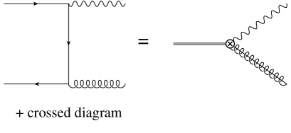
Figure 1: Matching onto SCET. The diagram on the left is calculated in full QCD, and then expanded in $\lambda$ and $v$. This is matched onto an operator in the EFT.

We next need to run using the SCET RGEs. This requires the anomalous dimensions of the operators. We therefore need to calculate the one-loop diagrams in Fig. 2. The anomalous dimensions of the ${}^{1}S_{0}$ and ${}^{3}P_{0}$ operators are the same, which is related to the fact that the Sudakov logs are the same for both channels [9]. Please see [4] for the details.

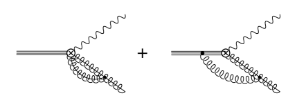
Figure 2: The one-loop diagrams needed to calculate the anomalous dimensions of the SCET operators.

We next match onto the soft theory, by removing all collinear particles. However, we have a collinear gluon in the final state, so to remove it, we perform an operator product expansion (OPE). The result is a non-local operator, separated along the light-cone. This is shown diagrammatically in Fig. 3.

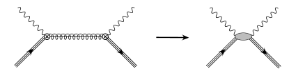
Figure 3: Matching onto the soft theory, by doing an OPE.

The operator we match onto is of the form

$$O_{n}(x)=\psi^{\dagger}\Gamma^{\prime n}\chi\delta(1-x+iD^{+}/M_{\Upsilon})\chi^{\dagger}\Gamma^{n}\psi,$$ (8)

where the derivative is in the $+$ light-like direction. The rate is now

$$\frac{d\Gamma}{dz}=\int dx\sum_{n}C_{n}(x-z)f_{n}(x)\langle O(n)\rangle,$$ (9)

where $f_{n}(x)=\langle O_{n}(x)\rangle/\langle O(n)\rangle$. This is just the rate including the shape function. By using SCET, the shape function appears naturally.

We now run down to the soft scale. For the details, see [4]. At this point, there are no large logs in the operators. We have summed all the Sudakov logs into the Wilson coefficients. To plot the result, we use the model of [13], introduced for $B$ decays. For $\Upsilon$, we need to give the shape function some unknown first moment of order $\Lambda_{\rm QCD}$ [4]. The results are shown in Fig. 4.

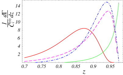
Figure 4: The differential decay spectra near the endpoint region in arbitrary units. The curves are described in the text.

The dashed curve is the resummation without the shape function. The dotted curve is the singular terms in the one-loop result, and the dot-dashed curve is these terms convoluted with the shape function. The solid curve is the resummation convoluted with the shape function. Note that the shape function without resummation and the resummation without the shape function give similar results. However, both are necessary.

At this point we compare to the color-singlet results. To do this we need the color-octet MEs. In Fig. 5, the solid curve is the color-singlet result. The dotted curve is the resummation without the shape function, the dashed is resummation with the shape function. The two sets of curves correspond to scaling the octet MEs from the singlet by factors of $v^{4}/10$ and $v^{4}/100$. As can be seen, to get comparable results, the naive scaling ($v^{4}$) seems to be off by a factor of 100 [14].

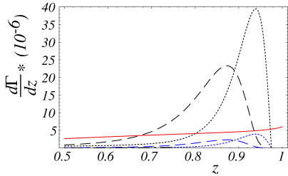
Figure 5: The different channels for the spectra near the endpoint region. The curves are described in the text.

However, before a meaningful comparison to the data is possible, we should follow a similar program for the color-singlet rate [12]. This will allow us to resum subleading Sudakov logs. The existence of these logs was first pointed out in [11], where it was observed that though the leading logs cancel in the color-singlet differential rate, they are present in the derivative of the rate.

References

- [1] G. T. Bodwin et al., Phys. Rev. D 51, 1125 (1995) [Erratum-ibid. D 55, 5853 (1997)].
- [2] M. Gremm and A. Kapustin, Phys. Lett. B 407, 323 (1997).
- [3] C. W. Bauer et al., Phys. Rev. D 63, 014006 (2001); see I. W. Stewart, these proceedings, and references therein.
- [4] C. W. Bauer et al., Phys. Rev. D 64, 114014 (2001).
- [5] S. J. Brodsky et al., Phys. Lett. B 73, 203 (1978); K. Koller and T. Walsh, Nucl. Phys. B 140, 449 (1978).
- [6] I. Z. Rothstein and M. B. Wise, Phys. Lett. B 402, 346 (1997).
- [7] M. Neubert, Phys. Rev. D 49, 4623 (1994); I. I. Bigi et al., Int. J. Mod. Phys. A 9, 2467 (1994); T. Mannel and M. Neubert, Phys. Rev. D 50, 2037 (1994).
- [8] M. Kramer, Phys. Rev. D 60, 111503 (1999).
- [9] F. Maltoni and A. Petrelli, Phys. Rev. D 59, 074006 (1999).
- [10] M. J. Dugan and B. Grinstein, Phys. Lett. B 255, 583 (1991).
- [11] F. Hautmann, Nucl. Phys. B 604, 391 (2001).
- [12] C. W. Bauer, S. Fleming and A. K. Leibovich, work in progress.
- [13] A. L. Kagan and M. Neubert, Eur. Phys. J. C 7, 5 (1999).
- [14] See, however, A. Petrelli et al., Nucl. Phys. B 514, 245 (1998).