New shifted hybrid inflation

Abstract:

A new shifted hybrid inflationary scenario is introduced which, in contrast to the older one, relies only on renormalizable superpotential terms. This scenario is automatically realized in a concrete extension of the ‘minimal’ supersymmetric Pati-Salam model which naturally leads to a moderate violation of Yukawa unification so that, for $\mu>0$, the predicted $b$-quark mass is acceptable even with universal boundary conditions. It is shown that this extended model possesses a classically flat ‘shifted’ trajectory which acquires a slope via one-loop radiative corrections and can be used as inflationary path. The constraints from the cosmic background explorer can be met with natural values of the relevant parameters. Also, there is no disastrous production of magnetic monopoles after inflation since the Pati-Salam gauge group is already broken on the ‘shifted’ path. The relevant part of inflation takes place at values of the inflaton field which are not much smaller than the ‘reduced’ Planck scale and, thus, supergravity corrections could easily invalidate inflation. It is, however, shown that inflation can be kept intact provided that an extra gauge singlet with a superheavy vacuum expectation value, which originates from D-terms, is introduced and a specific form of the Kähler potential is used. Moreover, it is found that, although the supergravity corrections are sizable, the constraints from the cosmic background explorer can again be met by readjusting the values of the parameters which were obtained with global supersymmetry.

1 Introduction

The recent measurements [1] of the three acoustic peaks of the angular power spectrum of the cosmic microwave background radiation (CMBR) have strongly favored the idea of inflation [2] (for a review see e.g., Ref.[3]). Moreover, inflation is now considered as the most likely explanation of the origin of structure formation in the universe. Therefore, it is important to construct viable models of inflation which are consistent with all particle physics and cosmological requirements. Undoubtedly, one of the most promising inflationary scenarios is hybrid inflation [4]. It uses two real scalar fields: a gauge non-singlet which provides the vacuum energy density needed for driving inflation and a gauge singlet which is the slowly varying field during inflation. Hybrid inflation is [5] naturally incorporated in supersymmetric (SUSY) grand unified theory (GUT) models based on gauge groups with rank greater than or equal to five (for specific successful models see e.g., Ref.[6]).

One of the most attractive rank five gauge groups is certainly the Pati-Salam (PS) group $G_{PS}=SU(4)_{c}\times SU(2)_{L}\times SU(2)_{R}$ [7]. This is the simplest GUT gauge group which can lead [8] to Yukawa unification [9]. It can also generate seesaw masses for the light neutrinos and has [10] many other interesting phenomenological implications. Moreover, SUSY PS GUT models are motivated [11] (see also Ref.[12]) from the recent D-brane setups and can also arise [13] from the standard weakly coupled heterotic string.

A characteristic feature of standard SUSY hybrid inflation, which is based on a renormalizable superpotential, is that the spontaneous breaking of the GUT gauge symmetry takes place at the end of inflation and thus topological defects may be copiously formed [14]. In particular, the spontaneous breaking of $G_{PS}$ to the standard model (SM) gauge group $G_{S}$ at the end of standard SUSY hybrid inflation leads [15] to the overproduction of topologically stable magnetic monopoles, which carry [16] two units of Dirac magnetic charge. So a cosmological disaster is encountered.

A way out of this potential catastrophe in hybrid inflationary models is to include into the standard superpotential for hybrid inflation the leading non-renormalizable term [15] (see also Ref.[14]; for a summary see Ref.[17]). It was observed [15] that this term cannot be excluded by any symmetry and can be comparable to the trilinear term of the standard superpotential. The coexistence of both these terms leads [15] to the appearance of a new ‘shifted’ classically flat valley of local minima where the GUT gauge symmetry is broken. This valley acquires a slope at the one-loop level and can be used [15] as an alternative inflationary path. In this scenario, which is known as shifted hybrid inflation, there is no formation of topological defects at the end of inflation and hence the potential monopole problem is avoided. This is crucial for the compatibility of the SUSY PS model with hybrid inflation since this model predicts the existence of magnetic monopoles.

It would be desirable to solve the (potential) magnetic monopole problem of hybrid inflation in SUSY GUTs with the GUT gauge group broken directly to $G_{S}$ without relying on the presence of non-renormalizable superpotential terms. (The monopole problem could also be solved by employing [18] an intermediate symmetry breaking scale or by other mechanisms (see e.g., Ref.[19]).) We shall, thus, examine the possibility of having shifted hybrid inflation in a SUSY PS GUT by using only renormalizable interactions and with $G_{PS}$ still broken to $G_{S}$ in a single step.

In this paper, we show that a new version of shifted hybrid inflation can take place in the SUSY PS model without invoking any non-renormalizable superpotential terms provided that we supplement the model with a new conjugate pair of superfields, $\phi$, $\bar{\phi}$, belonging to the representation (15,1,3) of $G_{PS}$. These fields lead to three new renormalizable terms in the part of the superpotential which is relevant for inflation.

This extension of the SUSY PS model is also motivated [20] by the requirement that Yukawa unification is moderately violated so that, for $\mu>0$, the predicted bottom quark mass resides within the experimentally allowed range even with universal boundary conditions. It is well-known [21] that, in models with Yukawa unification (or with large $\tan\beta$ in general), the $b$-quark mass receives large SUSY corrections which, for $\mu>0$, lead to unacceptably large values of $m_{b}$. The requirement that the SUSY correction to $m_{b}$ is not excessive imposes additional constraints on the parameter space and non-universal soft SUSY breaking terms as well as some deviation from the minimal Kähler potential must be considered [10, 22]. Another possible solution to this problem is to assume a small violation of Yukawa unification, which can be accommodated in the SUSY PS model by introducing new Higgs superfields as emphasized in Ref.[20]. It was shown that, in this case, one can get satisfactory values of $m_{b}$ even with universal boundary conditions and in accord with all other phenomenological and cosmological requirements.

This paper is organized as follows. In section 2, we consider the extended SUSY PS model and show that it possesses a ‘shifted’ classically flat direction. We then construct the mass spectrum on this trajectory and calculate the one-loop radiative corrections. We show that successful new shifted hybrid inflation can take place along this path where $G_{PS}$ is broken to $G_{S}$. Thus, the monopole problem is avoided. In section 3, we study the effect of supergravity (SUGRA) on inflation which, as it turns out, takes place at values of the inflaton field which are close to the ‘reduced’ Planck scale. We show that a mechanism [23] utilizing a specific Kähler potential can be used so that the SUGRA corrections do not invalidate inflation. However, the results which were obtained with global SUSY must now be readjusted. Our conclusions are summarized in section 4.

2 New shifted hybrid inflation

The SUSY PS model of Ref.[15] which leads to shifted hybrid inflation has been extended in Ref.[20] in order to allow a moderate violation of the ‘asymptotic’ Yukawa unification so that, for $\mu>0$, an acceptable value of the $b$-quark mass is obtained even with universal boundary conditions. We consider this extended model as the basis of our discussion here. The breaking of $G_{PS}$ to $G_{S}$ is achieved by the superheavy vacuum expectation values (VEVs) ($=M_{GUT}\approx 2.86\times 10^{16}~{}{\rm GeV}$, the SUSY GUT scale) of the right handed neutrino type components $\nu_{H}^{c}$, $\bar{\nu}_{H}^{c}$ of a conjugate pair of Higgs superfields $H^{c}=(\bar{4},1,2)$, $\bar{H}^{c}=(4,1,2)$. The model also contains a gauge singlet $S$ which triggers the breaking of $G_{PS}$. Finally, in order to have Yukawa unification violated by an amount which is adequate for $\mu>0$, a new conjugate pair of superfields $\phi$, $\bar{\phi}$ belonging to the (15,1,3) representation of $G_{PS}$ is included. For details on the full field content and superpotential, the global symmetries, the charge assignments, and the phenomenological and cosmological properties of this model, the reader is referred to Ref.[20] (and [15]).

The superpotential terms which are relevant for inflation are all renormalizable and are given by

$$W=\kappa S(H^{c}\bar{H}^{c}-M^{2})-\beta S\phi^{2}+m\phi\bar{\phi}+\lambda\bar{\phi}H^{c}\bar{H}^{c},$$ (1)

where $M$ and $m$ are superheavy masses of the order of $M_{GUT}$, and $\kappa$, $\beta$ and $\lambda$ are dimensionless coupling constants. These parameters are normalized so that they correspond to the couplings between the SM singlet components of the superfields. We can take $M,~{}m,~{}\kappa,~{}\lambda>0$ by field redefinitions. For simplicity, we also take $\beta>0$, although it can be generally complex.

The scalar potential obtained from $W$ is given by

$$V=\left|\kappa(H^{c}\bar{H}^{c}-M^{2})-\beta\phi^{2}\right|^{2}+\left|2\beta S\phi-m\bar{\phi}\right|^{2}+\left|m\phi+\lambda H^{c}\bar{H}^{c}\right|^{2}$$

$$+\left|\kappa S+\lambda\bar{\phi}\right|^{2}\left(|H^{c}|^{2}+|\bar{H}^{c}|^{2}\right)+{\rm D-terms},~{}~{}~{}~{}~{}~{}~{}~{}~{}~{}~{}~{}~{}~{}~{}~{}$$ (2)

where the complex scalar fields which belong to the SM singlet components of the superfields are denoted by the same symbols as the corresponding superfields. As usual, the vanishing of the D-terms yields $\bar{H}^{c}\,{}^{*}=e^{i\vartheta}H^{c}$ ($H^{c}$, $\bar{H}^{c}$ lie in the $\nu^{c}_{H}$, $\bar{\nu}^{c}_{H}$ direction). We restrict ourselves to the direction with $\vartheta=0$ which contains the ‘shifted’ inflationary path and the SUSY vacua (see below). Performing an appropriate global transformation, we can bring the complex scalar field $S$ to the positive real axis. Also, by a gauge transformation, the fields $H^{c}$, $\bar{H}^{c}$ can be made positive.

From the potential in Eq.(2), we find that the SUSY vacuum lies at

$$\frac{H^{c}\bar{H}^{c}}{M^{2}}\equiv\left(\frac{v_{0}}{M}\right)^{2}=\frac{1}{2\xi}\left(1-(1-4\xi)^{\frac{1}{2}}\right),~{}~{}S=0,~{}~{}\frac{\phi}{M}=-\frac{\kappa^{\frac{1}{2}}\xi^{\frac{1}{2}}}{\beta^{\frac{1}{2}}}\left(\frac{v_{0}}{M}\right)^{2},~{}~{}\bar{\phi}=0,$$ (3)

where $\xi=\beta\lambda^{2}M^{2}/\kappa m^{2}<1/4$. Here, we chose the vacuum with the smallest $v_{0}~{}(>0)$ for the same reasons as in Ref.[15]. The potential possesses the trivial flat direction at $H^{c}=\bar{H}^{c}=\phi=\bar{\phi}=0$ with $V=\kappa^{2}M^{4}$. It also possesses a ‘shifted’ flat direction at

$$\frac{H^{c}\bar{H}^{c}}{M^{2}}\equiv\left(\frac{v}{M}\right)^{2}=\frac{2\kappa^{2}(\frac{1}{4\xi}+1)+\frac{\lambda^{2}}{\xi}}{2(\kappa^{2}+\lambda^{2})},~{}~{}S>0,~{}~{}\frac{\phi}{M}=-\frac{\kappa^{\frac{1}{2}}}{2\beta^{\frac{1}{2}}\xi^{\frac{1}{2}}},~{}~{}\bar{\phi}=-\frac{\kappa}{\lambda}S$$ (4)

with

$$\frac{V_{0}}{M^{4}}=\frac{\kappa^{2}\lambda^{2}}{\kappa^{2}+\lambda^{2}}\left(\frac{1}{4\xi}-1\right)^{2},$$ (5)

which can be used as inflationary path. As in the case of the shifted hybrid inflationary model of Ref.[15], which is based on non-renormalizable superpotential terms, the constant classical energy density on the ‘shifted’ path breaks SUSY, while the constant non-zero values of $H^{c}$, $\bar{H}^{c}$ break the GUT gauge symmetry. The SUSY breaking implies the existence of one-loop radiative corrections which lift the classical flatness of this path yielding the necessary inclination for driving the inflaton towards the SUSY vacuum.

The one-loop radiative corrections to the potential along the ‘shifted’ inflationary trajectory are calculated by using the Coleman-Weinberg formula [24]:

$$\Delta V=\frac{1}{64\pi^{2}}\sum_{i}(-)^{F_{i}}M_{i}^{4}\ln\frac{M_{i}^{2}}{\Lambda^{2}},$$ (6)

where the sum extends over all helicity states $i$, $F_{i}$ and $M_{i}^{2}$ are the fermion number and mass squared of the $i$th state and $\Lambda$ is a renormalization mass scale. In order to use this formula for creating a logarithmic slope which drives the inflaton towards the minimum, one has first to derive the mass spectrum of the model on the ‘shifted’ inflationary path.

As mentioned, during inflation, $H^{c}$, $\bar{H}^{c}$ acquire constant values in the $\nu_{H}^{c}$, $\bar{\nu}_{H}^{c}$ directions which are equal to $v~{}(>0)$ and break $G_{PS}$ to $G_{S}$. We can then write $\nu^{c}_{H}=v+\delta\nu^{c}_{H}$, $\bar{\nu}^{c}_{H}=v+\delta\bar{\nu}^{c}_{H}$, where $\delta\nu^{c}_{H}$, $\delta\bar{\nu}^{c}_{H}$ are complex scalar fields. The (complex) deviations of the fields $S$, $\phi$, $\bar{\phi}$ from their values at a point on the ‘shifted’ path (corresponding to $S>0$) are similarly denoted as $\delta S$, $\delta\phi$, $\delta\bar{\phi}$. We define the complex scalar fields

$$\theta = \frac{\delta\nu_{H}^{c}+\delta\bar{\nu}^{c}_{H}}{\sqrt{2}},~{}~{}~{}~{}~{}\eta=\frac{\delta\nu_{H}^{c}-\delta\bar{\nu}^{c}_{H}}{\sqrt{2}},$$ (7)

$$\zeta = \frac{\kappa\delta S+\lambda\delta\bar{\phi}}{(\kappa^{2}+\lambda^{2})^{\frac{1}{2}}},~{}~{}~{}~{}~{}~{}\varepsilon=\frac{\lambda\delta S-\kappa\delta\bar{\phi}}{(\kappa^{2}+\lambda^{2})^{\frac{1}{2}}}\cdot$$ (8)

We find that $\eta$ and $\varepsilon$ do not acquire any masses from the scalar potential in Eq.(2). Actually, $\varepsilon$ (and its SUSY partner) remains massless even after including the gauge interactions (see below). It corresponds to the complex inflaton field $\Sigma=(\lambda S-\kappa\bar{\phi})/(\kappa^{2}+\lambda^{2})^{1/2}$, which on the ‘shifted’ path takes the form $\Sigma=(\kappa^{2}+\lambda^{2})^{1/2}S/\lambda$. So, in this case, the real normalized inflaton field is $\sigma=2^{1/2}(\kappa^{2}+\lambda^{2})^{1/2}S/\lambda$.

Contrary to $\eta$ and $\varepsilon$, the complex scalars $\theta$, $\delta\phi$ and $\zeta$ acquire masses from the potential in Eq.(2). Expanding these scalars in real and imaginary parts $\theta=(\theta_{1}+i\theta_{2})/\sqrt{2}$, $\delta\phi=(\delta\phi_{1}+i\delta\phi_{2})/\sqrt{2}$, $\zeta=(\zeta_{1}+i\zeta_{2})/\sqrt{2}$, we find that the mass squared matrices $M_{+}^{2}$ and $M_{-}^{2}$ of $\theta_{1}$, $\delta\phi_{1}$, $\zeta_{1}$ and $\theta_{2}$, $\delta\phi_{2}$, $\zeta_{2}$ are given by

$$M_{\pm}^{2}=M^{2}\left(\begin{array}[]{ccc}a^{2}&~{}~{}ab&~{}~{}0\\ ab&~{}~{}b^{2}+c^{2}\pm f^{2}&~{}~{}-cb\\ 0&~{}~{}-cb&~{}~{}a^{2}+b^{2}\end{array}\right),$$ (9)

where $a^{2}=2\kappa^{2}(1/4\xi+1)+\lambda^{2}/\xi$, $b^{2}=\beta(\kappa^{2}+\lambda^{2})/\kappa\xi$, $c^{2}=2\beta^{2}\lambda^{2}\sigma^{2}/M^{2}(\kappa^{2}+\lambda^{2})$, $f^{2}=2\kappa\beta\lambda^{2}(1/4\xi-1)/(\kappa^{2}+\lambda^{2})$ ($a$, $b$, $c$, $f>0$).

One can show that, for $\sigma\to\infty$ ($c\to\infty$), all the eigenvalues of these two mass squared matrices are positive. So, for large values of $\sigma$, the ‘shifted’ path is a valley of local minima. As $\sigma$ decreases, one eigenvalue may become negative destabilizing the trajectory. From continuity, no eigenvalue can become negative without passing from zero. So, the critical (instability) point on the ‘shifted’ trajectory is encountered when one of the determinants of the matrices in Eq.(9), which are $\det M_{\pm}^{2}=M^{6}a^{2}(a^{2}c^{2}\pm f^{2}(a^{2}+b^{2}))$, vanishes. We see that $\det M_{+}^{2}$ is always positive, while $\det M_{-}^{2}$ vanishes at $c^{2}=f^{2}(1+b^{2}/a^{2})$, which corresponds to the critical point of the ‘shifted’ path given by

$$\left(\frac{\sigma_{c}}{M}\right)^{2}=\frac{\kappa}{\beta}\left(\frac{1}{4\xi}-1\right)\frac{2\kappa^{2}\left(1+\frac{\kappa+2\beta}{4\kappa\xi}\right)+\frac{\lambda^{2}(\kappa+\beta)}{\kappa\xi}}{2\kappa^{2}\left(1+\frac{1}{4\xi}\right)+\frac{\lambda^{2}}{\xi}}\cdot$$ (10)

The superpotential in Eq.(1) gives rise to mass terms between the fermionic partners of $\theta$, $\delta\phi$ and $\zeta$. The square of the corresponding mass matrix is found to be

$$M_{0}^{2}=M^{2}\left(\begin{array}[]{ccc}a^{2}&~{}~{}ab&~{}~{}0\\ ab&~{}~{}b^{2}+c^{2}&~{}~{}-cb\\ 0&~{}~{}-cb&~{}~{}a^{2}+b^{2}\end{array}\right).$$ (11)

To complete the spectrum in the SM singlet sector, which consists of the superfields $\nu^{c}_{H}$, $\bar{\nu}^{c}_{H}$, $S$, $\phi$ and $\bar{\phi}$ (SM singlet directions), we must consider the following D-terms in the scalar potential:

$$\frac{1}{2}g^{2}\sum_{a}(H^{c}\,{}^{*}T^{a}H^{c}+\bar{H}^{c}\,{}^{*}T^{a}\bar{H}^{c})^{2},$$ (12)

where $g$ is the $G_{PS}$ gauge coupling constant and the sum extends over all the generators $T^{a}$ of $G_{PS}$. The part of this sum over the generators $T^{15}=(1/2\sqrt{6})~{}\mathrm{diag}(1,1,1,-3)$ of $SU(4)_{c}$ and $T^{3}=(1/2)~{}\mathrm{diag}(1,-1)$ of $SU(2)_{R}$ gives rise to a mass term for the normalized real scalar field $\eta_{1}$ with $m^{2}=5g^{2}v^{2}/2$. The field $\eta_{2}$, however, is left massless by the D-terms and is absorbed by the gauge boson $A^{\perp}=-(3/5)^{1/2}A^{15}+(2/5)^{1/2}A^{3}$ which becomes massive with $m^{2}=5g^{2}v^{2}/2$ ($A^{15}$, $A^{3}$ are the gauge bosons corresponding to $T^{15}$, $T^{3}$).

Contributions to the fermion masses also arise from the Lagrangian terms

$$i\sqrt{2}g\sum_{a}\lambda^{a}(H^{c}\,{}^{*}T^{a}\psi_{H^{c}}+\bar{H}^{c}\,{}^{*}T^{a}\psi_{\bar{H}^{c}})+{\rm h.c.},$$ (13)

where $\lambda^{a}$ is the gaugino corresponding to $T^{a}$ and $\psi_{H^{c}}$, $\psi_{\bar{H}^{c}}$ represent the chiral fermions in the superfields $H^{c}$, $\bar{H}^{c}$. Concentrating again on $T^{15}$, $T^{3}$, we obtain a Dirac mass term between the chiral fermion in the $\eta$ direction and $-i\lambda^{\perp}$ (with $\lambda^{\perp}$ being the SUSY partner of $A^{\perp}$) with $m^{2}=5g^{2}v^{2}/2$. Note that the SM singlet components of $\phi$ and $\bar{\phi}$ do not contribute to bosonic and fermionic couplings analogous to the ones in Eqs.(12) and (13) since they commute with $T^{15}$ and $T^{3}$.

This completes the analysis of the SM singlet sector of the model. In summary, we found two groups of three real scalars with mass squared matrices $M_{\pm}^{2}$ and three two component fermions with mass matrix squared $M_{0}^{2}$. Also, one Dirac fermion (with four components), one gauge boson and one real scalar, all of them having the same mass squared $m^{2}=5g^{2}v^{2}/2$ and, thus, not contributing to the one-loop radiative corrections. From Eq.(6), we find that the contribution of the SM singlet sector to the radiative corrections to the potential along the ‘shifted’ path is given by

$$\Delta V=\frac{1}{64\pi^{2}}{\rm Tr}\left(M_{+}^{4}\ln\frac{M_{+}^{2}}{\Lambda^{2}}+M_{-}^{4}\ln\frac{M_{-}^{2}}{\Lambda^{2}}-2M_{0}^{4}\ln\frac{M_{0}^{2}}{\Lambda^{2}}\right)\cdot$$ (14)

One can show that, in this sector, ${\rm Tr}M^{2}=0$ and ${\rm Tr}M^{4}=2M^{4}f^{4}$, which is $\sigma$-independent and, thus, the generated slope on the ‘shifted’ path is $\Lambda$-independent.

We now turn to the $u^{c}$ and $\bar{u}^{c}$ type fields which are color antitriplets with charge $-2/3$ and color triplets with charge $2/3$ respectively. Such fields exist in $H^{c}$, $\bar{H}^{c}$, $\phi$ and $\bar{\phi}$, and we shall denote them by $u^{c}_{H}$, $\bar{u}^{c}_{H}$, $u^{c}_{\phi}$, $\bar{u}^{c}_{\phi}$, $u^{c}_{\bar{\phi}}$ and $\bar{u}^{c}_{\bar{\phi}}$. The relevant expansion of $\phi$ is

$$\phi=\left[\frac{1}{\sqrt{12}}\left(\begin{array}[]{cccc}1&~{}0&~{}0&~{}0\\ 0&~{}1&~{}0&~{}0\\ 0&~{}0&~{}1&~{}0\\ 0&~{}0&~{}0&-3\end{array}\right),~{}\frac{1}{\sqrt{2}}\left(\begin{array}[]{cc}1&~{}0\\ 0&-1\end{array}\right)\right]\phi+\left(\begin{array}[]{cccc}0&~{}0&~{}0&~{}0\\ 0&~{}0&~{}0&~{}0\\ 0&~{}0&~{}0&~{}0\\ 1&~{}0&~{}0&~{}0\\ \end{array}\right)u^{c}_{\phi}+\left(\begin{array}[]{cccc}0&~{}0&~{}0&~{}1\\ 0&~{}0&~{}0&~{}0\\ 0&~{}0&~{}0&~{}0\\ 0&~{}0&~{}0&~{}0\\ \end{array}\right)\bar{u}^{c}_{\phi}+\cdots,$$ (15)

where the SM singlet in $\phi$ (denoted by the same symbol) is also shown with the first (second) matrix in the brackets belonging to the algebra of $SU(4)_{c}$ ($SU(2)_{R}$). The fields $u^{c}_{\phi}$, $\bar{u}^{c}_{\phi}$ are $SU(2)_{R}$ singlets, so only their $SU(4)_{c}$ structure is shown and summation over their $SU(3)_{c}$ indices is implied in the ellipsis. The field $\bar{\phi}$ can be similarly expanded.

In the bosonic $u^{c}$, $\bar{u}^{c}$ type sector, we find that the mass squared matrices $m(u)_{\pm}^{2}$ of the complex scalars $u_{H\pm}^{c}=(u_{H}^{c}\pm\bar{u}^{c~{}*}_{H})/\sqrt{2}$, $u_{\phi\pm}^{c}=(u_{\phi}^{c}\pm\bar{u}^{c~{}*}_{\phi})/\sqrt{2}$ and $u_{\bar{\phi}\pm}^{c}=(u_{\bar{\phi}}^{c}\pm\bar{u}_{\bar{\phi}}^{c~{}*})/\sqrt{2}$ are given by

$$m(u)_{+}^{2}=M^{2}\left(\begin{array}[]{ccc}\frac{4\kappa^{2}c^{2}}{9\beta^{2}}+\frac{2\lambda^{2}a^{2}\beta}{3\kappa\xi b^{2}}+\frac{2\kappa f^{2}}{3\beta}&~{}~{}-\frac{\sqrt{2}\lambda^{2}\beta a}{\sqrt{3}\kappa\xi b}&~{}~{}-\frac{2\sqrt{2}\kappa^{\frac{1}{2}}\lambda ca}{3\sqrt{3}\beta^{\frac{1}{2}}\xi^{\frac{1}{2}}b}\\ -\frac{\sqrt{2}\lambda^{2}\beta a}{\sqrt{3}\kappa\xi b}&~{}~{}\frac{\beta\lambda^{2}}{\kappa\xi}+c^{2}-f^{2}&~{}~{}-\frac{\lambda\beta^{\frac{1}{2}}c}{\kappa^{\frac{1}{2}}\xi^{\frac{1}{2}}}\\ -\frac{2\sqrt{2}\kappa^{\frac{1}{2}}\lambda ca}{3\sqrt{3}\beta^{\frac{1}{2}}\xi^{\frac{1}{2}}b}&~{}~{}-\frac{\lambda\beta^{\frac{1}{2}}c}{\kappa^{\frac{1}{2}}\xi^{\frac{1}{2}}}&~{}~{}~{}\frac{\beta\lambda^{2}}{\kappa\xi}+\frac{2\lambda^{2}a^{2}\beta}{3\kappa\xi b^{2}}\end{array}\right)$$ (16)

and

$$m(u)_{-}^{2}=M^{2}\left(\!\begin{array}[]{ccc}\frac{4\kappa^{2}c^{2}}{9\beta^{2}}\!+\!\frac{2\lambda^{2}a^{2}\beta}{3\kappa\xi b^{2}}\!-\!\frac{2\kappa f^{2}}{3\beta}\!+\!\frac{g^{2}a^{2}\beta}{2\kappa\xi b^{2}}\!\!&\frac{-\sqrt{2}\lambda^{2}\beta a}{\sqrt{3}\kappa\xi b}\!+\!\frac{g^{2}a}{\sqrt{6}\xi b}\!\!&\frac{-2\sqrt{2}\kappa^{\frac{1}{2}}\lambda ca}{3\sqrt{3}\beta^{\frac{1}{2}}\xi^{\frac{1}{2}}b}\!+\!\frac{g^{2}\kappa^{\frac{1}{2}}ac}{\sqrt{6}\xi^{\frac{1}{2}}\beta^{\frac{1}{2}}\lambda b}\\ \!\frac{-\sqrt{2}\lambda^{2}\beta a}{\sqrt{3}\kappa\xi b}\!+\!\frac{g^{2}a}{\sqrt{6}\xi b}\!\!&\frac{\beta\lambda^{2}}{\kappa\xi}\!+\!c^{2}\!+\!f^{2}\!+\!\frac{g^{2}\kappa}{3\beta\xi}\!\!&\!\frac{-\lambda\beta^{\frac{1}{2}}c}{\kappa^{\frac{1}{2}}\xi^{\frac{1}{2}}}\!+\!\frac{g^{2}c\kappa^{\frac{3}{2}}}{3\xi^{\frac{1}{2}}\beta^{\frac{3}{2}}\lambda}\\ \!\frac{-2\sqrt{2}\kappa^{\frac{1}{2}}\lambda ca}{3\sqrt{3}\beta^{\frac{1}{2}}\xi^{\frac{1}{2}}b}\!+\!\frac{g^{2}\kappa^{\frac{1}{2}}ac}{\sqrt{6}\xi^{\frac{1}{2}}\beta^{\frac{1}{2}}\lambda b}\!\!&\!\frac{-\lambda\beta^{\frac{1}{2}}c}{\kappa^{\frac{1}{2}}\xi^{\frac{1}{2}}}\!+\!\frac{g^{2}c\kappa^{\frac{3}{2}}}{3\xi^{\frac{1}{2}}\beta^{\frac{3}{2}}\lambda}\!\!&\frac{\beta\lambda^{2}}{\kappa\xi}\!+\!\frac{2\lambda^{2}a^{2}\beta}{3\kappa\xi b^{2}}\!+\!\frac{g^{2}\kappa^{2}c^{2}}{3\lambda^{2}\beta^{2}}\end{array}\!\right).$$ (17)

The mass squared matrix $m(u)^{2}_{+}$ has one zero eigenvalue corresponding to the Goldstone boson which is absorbed by the superhiggs mechanism. This is easily checked by showing that $\det m(u)_{+}^{2}=0$. However, it does no harm to keep this Goldstone mode since it has vanishing contribution to the radiative corrections in Eq.(6) anyway.

In the $u^{c}$, $\bar{u}^{c}$ type sector, we obtain four Dirac fermions (per color) $\psi^{D}_{u^{c}}=\psi_{u^{c}}+\psi_{\bar{u}^{c}}^{c}$, $\psi^{D}_{u^{c}_{\phi}}=\psi_{u^{c}_{\phi}}+\psi^{c}_{\bar{u}^{c}_{\phi}}$, $\psi^{D}_{u^{c}_{\bar{\phi}}}=\psi_{u^{c}_{\bar{\phi}}}+\psi^{c}_{\bar{u}^{c}_{\bar{\phi}}}$, $-i\lambda^{D}=-i(\lambda^{+}+\lambda^{-~{}c})$. Here, $\lambda^{\pm}=(\lambda^{1}\pm i\lambda^{2})/\sqrt{2}$, where $\lambda^{1}$ ($\lambda^{2}$) is the gaugino color triplet corresponding to the $SU(4)_{c}$ generators with $1/2$ ($-i/2$) in the $i4$ and $1/2$ ($i/2$) in the $4i$ entry ($i=1,2,3$). The fermionic mass matrix is

$$m(\psi_{u})=M\left(\begin{array}[]{cccc}\frac{2\kappa c}{3\beta}&~{}~{}0&~{}~{}-\frac{\sqrt{2}\beta^{\frac{1}{2}}\lambda a}{\sqrt{3}\kappa^{\frac{1}{2}}\xi^{\frac{1}{2}}b}&~{}~{}\frac{ga\beta^{\frac{1}{2}}}{\sqrt{2}\kappa^{\frac{1}{2}}\xi^{\frac{1}{2}}b}\\ 0&~{}~{}-c&~{}~{}\frac{\beta^{\frac{1}{2}}\lambda}{\kappa^{\frac{1}{2}}\xi^{\frac{1}{2}}}&~{}~{}\frac{g\kappa^{\frac{1}{2}}}{\sqrt{3}\beta^{\frac{1}{2}}\xi^{\frac{1}{2}}}\\ -\frac{\sqrt{2}\beta^{\frac{1}{2}}\lambda a}{\sqrt{3}\kappa^{\frac{1}{2}}\xi^{\frac{1}{2}}b}&~{}~{}\frac{\beta^{\frac{1}{2}}\lambda}{\kappa^{\frac{1}{2}}\xi^{\frac{1}{2}}}&~{}~{}0&~{}~{}\frac{g\kappa c}{\sqrt{3}\lambda\beta}\\ \frac{ga\beta^{\frac{1}{2}}}{\sqrt{2}\kappa^{\frac{1}{2}}\xi^{\frac{1}{2}}b}&~{}~{}\frac{g\kappa^{\frac{1}{2}}}{\sqrt{3}\beta^{\frac{1}{2}}\xi^{\frac{1}{2}}}&~{}~{}\frac{g\kappa c}{\sqrt{3}\lambda\beta}&~{}~{}0\end{array}\right).$$ (18)

To complete this sector, we must also include the gauge bosons $A^{\pm}$ which are associated with $\lambda^{\pm}$. They acquire a mass squared $m^{2}_{g}=g^{2}M^{2}(a^{2}\beta/2\kappa\xi b^{2}+\kappa/3\beta\xi+\kappa^{2}c^{2}/3\beta^{2}\lambda^{2})$.

The overall contribution of the $u^{c}$, $\bar{u}^{c}$ type sector to $\Delta V$ in Eq.(6) is

$$\Delta V=\frac{3}{32\pi^{2}}{\rm Tr}\left(m(u)^{4}_{+}\ln\frac{m(u)_{+}^{2}}{\Lambda^{2}}+m(u)^{4}_{-}\ln\frac{m(u)_{-}^{2}}{\Lambda^{2}}-2m(\psi_{u})^{4}\ln\frac{m(\psi_{u})^{2}}{\Lambda^{2}}+3m_{g}^{4}\ln\frac{m_{g}^{2}}{\Lambda^{2}}\right).$$ (19)

In this sector, ${\rm Tr}M^{2}=0$ and ${\rm Tr}M^{4}=12M^{4}f^{4}(1+4\kappa^{2}/9\beta^{2}-2g^{2}\kappa^{2}/3\beta^{2}\lambda^{2})$. So, the contribution of this sector to the slope of the ‘shifted’ path is also $\Lambda$-independent.

We will now discuss the contribution from the $e^{c}$, $\bar{e}^{c}$ type sector consisting of color singlets with charge $1$, $-1$. Such fields exist in $H^{c}$, $\bar{H}^{c}$, $\phi$, $\bar{\phi}$ and we denote them by $e^{c}_{H}$, $\bar{e}^{c}_{H}$, $e^{c}_{\phi}$, $\bar{e}^{c}_{\phi}$, $e^{c}_{\bar{\phi}}$, $\bar{e}^{c}_{\bar{\phi}}$. The field $\phi$ can be expanded in $e^{c}_{\phi}$, $\bar{e}^{c}_{\phi}$ as follows:

$$\phi=\left[\frac{1}{\sqrt{12}}\left(\begin{array}[]{cccc}1&~{}0&~{}0&~{}0\\ 0&~{}1&~{}0&~{}0\\ 0&~{}0&~{}1&~{}0\\ 0&~{}0&~{}0&-3\end{array}\right),~{}\left(\begin{array}[]{cc}0&~{}1\\ 0&~{}0\end{array}\right)e^{c}_{\phi}+\left(\begin{array}[]{cc}0&~{}0\\ 1&~{}0\end{array}\right)\bar{e}^{c}_{\phi}\right]+\cdots,$$ (20)

with the same notation as in Eq.(15). A similar expansion holds for $\bar{\phi}$. The analysis in this sector is similar to the one in the $u^{c}$, $\bar{u}^{c}$ type sector and we only summarize the results.

In the bosonic sector, we obtain two groups each consisting of three complex scalars with mass squared matrices

$$m(e)_{+}^{2}=M^{2}\left(\begin{array}[]{ccc}\frac{\kappa^{2}c^{2}}{\beta^{2}}+\frac{\lambda^{2}a^{2}\beta}{\kappa\xi b^{2}}+\frac{\kappa f^{2}}{\beta}&~{}~{}\frac{\lambda^{2}\beta a}{\kappa\xi b}&~{}~{}\frac{\kappa^{\frac{1}{2}}\lambda ca}{\beta^{\frac{1}{2}}\xi^{\frac{1}{2}}b}\\ \frac{\lambda^{2}\beta a}{\kappa\xi b}&~{}~{}\frac{\beta\lambda^{2}}{\kappa\xi}+c^{2}-f^{2}&~{}~{}-\frac{\lambda\beta^{\frac{1}{2}}c}{\kappa^{\frac{1}{2}}\xi^{\frac{1}{2}}}\\ \frac{\kappa^{\frac{1}{2}}\lambda ca}{\beta^{\frac{1}{2}}\xi^{\frac{1}{2}}b}&~{}~{}-\frac{\lambda\beta^{\frac{1}{2}}c}{\kappa^{\frac{1}{2}}\xi^{\frac{1}{2}}}&~{}~{}\frac{\beta\lambda^{2}}{\kappa\xi}+\frac{\lambda^{2}a^{2}\beta}{\kappa\xi b^{2}}\end{array}\right)$$ (21)

and

$$m(e)_{-}^{2}=M^{2}\left(\!\begin{array}[]{ccc}\frac{\kappa^{2}c^{2}}{\beta^{2}}\!+\!\frac{\lambda^{2}a^{2}\beta}{\kappa\xi b^{2}}\!-\!\frac{\kappa f^{2}}{\beta}\!+\!\frac{g^{2}a^{2}\beta}{2\kappa\xi b^{2}}\!\!&\frac{\lambda^{2}\beta a}{\kappa\xi b}\!-\!\frac{g^{2}a}{2\xi b}\!\!&\frac{\kappa^{\frac{1}{2}}\lambda ca}{\beta^{\frac{1}{2}}\xi^{\frac{1}{2}}b}\!-\!\frac{g^{2}\kappa^{\frac{1}{2}}ac}{2\xi^{\frac{1}{2}}\beta^{\frac{1}{2}}\lambda b}\\ \!\frac{\lambda^{2}\beta a}{\kappa\xi b}\!-\!\frac{g^{2}a}{2\xi b}\!\!&\frac{\beta\lambda^{2}}{\kappa\xi}\!+\!c^{2}\!+\!f^{2}\!+\!\frac{g^{2}\kappa}{2\xi\beta}\!\!&\!\frac{-\lambda\beta^{\frac{1}{2}}c}{\kappa^{\frac{1}{2}}\xi^{\frac{1}{2}}}\!+\!\frac{g^{2}\kappa^{\frac{3}{2}}c}{2\xi^{\frac{1}{2}}\beta^{\frac{3}{2}}\lambda}\\ \!\frac{\kappa^{\frac{1}{2}}\lambda ca}{\beta^{\frac{1}{2}}\xi^{\frac{1}{2}}b}\!-\!\frac{g^{2}\kappa^{\frac{1}{2}}ac}{2\xi^{\frac{1}{2}}\beta^{\frac{1}{2}}\lambda b}\!\!&\!\frac{-\lambda\beta^{\frac{1}{2}}c}{\kappa^{\frac{1}{2}}\xi^{\frac{1}{2}}}\!+\!\frac{g^{2}\kappa^{\frac{3}{2}}c}{2\xi^{\frac{1}{2}}\beta^{\frac{3}{2}}\lambda}\!\!&\frac{\beta\lambda^{2}}{\kappa\xi}\!+\!\frac{\lambda^{2}a^{2}\beta}{\kappa\xi b^{2}}\!+\!\frac{g^{2}\kappa^{2}c^{2}}{2\lambda^{2}\beta^{2}}\end{array}\!\right).$$ (22)

The matrix $m(e)^{2}_{+}$, similarly to $m(u)^{2}_{+}$ in the $u^{c}$, $\bar{u}^{c}$ type sector, has one zero eigenvalue corresponding to the Goldstone mode absorbed by the superhiggs mechanism.

In the fermion sector, we obtain four Dirac fermions with mass matrix given by

$$m(\psi_{e})=M\left(\begin{array}[]{cccc}\frac{\kappa c}{\beta}&~{}~{}0&~{}~{}\frac{\beta^{\frac{1}{2}}\lambda a}{\kappa^{\frac{1}{2}}\xi^{\frac{1}{2}}b}&~{}~{}\frac{ga\beta^{\frac{1}{2}}}{\sqrt{2}\kappa^{\frac{1}{2}}\xi^{\frac{1}{2}}b}\\ 0&~{}~{}-c&~{}~{}\frac{\beta^{\frac{1}{2}}\lambda}{\kappa^{\frac{1}{2}}\xi^{\frac{1}{2}}}&~{}~{}-\frac{g\kappa^{\frac{1}{2}}}{\sqrt{2}\beta^{\frac{1}{2}}\xi^{\frac{1}{2}}}\\ \frac{\beta^{\frac{1}{2}}\lambda a}{\kappa^{\frac{1}{2}}\xi^{\frac{1}{2}}b}&~{}~{}\frac{\beta^{\frac{1}{2}}\lambda}{\kappa^{\frac{1}{2}}\xi^{\frac{1}{2}}}&~{}~{}0&~{}~{}-\frac{g\kappa c}{\sqrt{2}\lambda\beta}\\ \frac{ga\beta^{\frac{1}{2}}}{\sqrt{2}\kappa^{\frac{1}{2}}\xi^{\frac{1}{2}}b}&~{}~{}-\frac{g\kappa^{\frac{1}{2}}}{\sqrt{2}\beta^{\frac{1}{2}}\xi^{\frac{1}{2}}}&~{}~{}-\frac{g\kappa c}{\sqrt{2}\lambda\beta}&~{}~{}0\end{array}\right).$$ (23)

We also have, in this sector, one complex gauge boson with mass squared given by $\hat{m}_{g}^{2}=g^{2}M^{2}(a^{2}\beta/2\kappa\xi b^{2}+\kappa/2\beta\xi+\kappa^{2}c^{2}/2\beta^{2}\lambda^{2})$.

The contribution of the $e^{c}$, $\bar{e}^{c}$ type sector to $\Delta V$ is

$$\Delta V=\frac{1}{32\pi^{2}}{\rm Tr}\left(m(e)^{4}_{+}\ln\frac{m(e)_{+}^{2}}{\Lambda^{2}}+m(e)^{4}_{-}\ln\frac{m(e)_{-}^{2}}{\Lambda^{2}}-2m(\psi_{e})^{4}\ln\frac{m(\psi_{e})^{2}}{\Lambda^{2}}+3\hat{m}_{g}^{4}\ln\frac{\hat{m}_{g}^{2}}{\Lambda^{2}}\right).$$ (24)

One can show that ${\rm Tr}M^{2}=0$ and ${\rm Tr}M^{4}=4M^{4}f^{4}(1+\kappa^{2}/\beta^{2}-g^{2}\kappa^{2}/\beta^{2}\lambda^{2})$ in this sector and, thus, its contribution to the inflationary slope is again $\Lambda$-independent.

We next consider the $d^{c}$ and $\bar{d}^{c}$ type sector consisting of color antitriplets with charge $1/3$ and color triplets with charge $-1/3$. We have the fields $d^{c}_{H}$, $\bar{d}^{c}_{H}$ from $H^{c}$, $\bar{H}^{c}$ and the fields $d^{c}_{\phi}$, $\bar{d}^{c}_{\phi}$, $d^{c}_{\bar{\phi}}$, $\bar{d}^{c}_{\bar{\phi}}$ from $\phi$, $\bar{\phi}$. Note that $\phi$ can be expanded as

$$\phi=\left[\left(\begin{array}[]{cccc}0&~{}0&~{}0&~{}0\\ 0&~{}0&~{}0&~{}0\\ 0&~{}0&~{}0&~{}0\\ 1&~{}0&~{}0&~{}0\end{array}\right),\left(\begin{array}[]{cc}0&~{}1\\ 0&~{}0\end{array}\right)\right]d^{c}_{\phi}+\left[\left(\begin{array}[]{cccc}0&~{}0&~{}0&~{}1\\ 0&~{}0&~{}0&~{}0\\ 0&~{}0&~{}0&~{}0\\ 0&~{}0&~{}0&~{}0\end{array}\right),\left(\begin{array}[]{cc}0&~{}0\\ 1&~{}0\end{array}\right)\right]\bar{d}^{c}_{\phi}+\cdots,$$ (25)

with the notation of Eq.(15). The field $\bar{\phi}$ is similarly expanded. In order to give superheavy masses to $d^{c}_{H}$ and $\bar{d}^{c}_{H}$, we introduce [13] a $SU(4)_{c}$ 6-plet superfield $G=(6,1,1)$ with the superpotential couplings $xGH^{c}H^{c}$, $yG\bar{H}^{c}\bar{H}^{c}$. The field $G$ splits, under $G_{S}$, into $g^{c}=(\bar{3},1,1/3)$ and $\bar{g}^{c}=(3,1,-1/3)$.

The mass terms of the complex scalars $d^{c}_{H}$, $\bar{d}^{c}_{H}$, $d^{c}_{\phi}$, $\bar{d}^{c}_{\phi}$, $d^{c}_{\bar{\phi}}$, $\bar{d}^{c}_{\bar{\phi}}$, $g^{c}$, $\bar{g}^{c}$ are

$$\mathcal{L}_{m}(d) = M^{2}\Big{[}\Big{(}\frac{\kappa^{2}c^{2}}{9\beta^{2}}+\frac{2a^{2}\beta}{\kappa\xi b^{2}}\Big{(}\frac{2\lambda^{2}}{3}+x^{2}\Big{)}\Big{)}|d^{c}_{H}|^{2}+\Big{(}\frac{\kappa^{2}c^{2}}{9\beta^{2}}+\frac{2a^{2}\beta}{\kappa\xi b^{2}}\Big{(}\frac{2\lambda^{2}}{3}+y^{2}\Big{)}\Big{)}|\bar{d}^{c}_{H}|^{2}$$ (26)

$$+ \Big{(}\frac{\beta\lambda^{2}}{\kappa\xi}+c^{2}\Big{)}(|d^{c}_{\phi}|^{2}+|\bar{d}^{c}_{\phi}|^{2})+\Big{(}\frac{\beta\lambda^{2}}{\kappa\xi}+\frac{4\lambda^{2}a^{2}\beta}{3\kappa\xi b^{2}}\Big{)}(|d^{c}_{\bar{\phi}}|^{2}+|\bar{d}^{c}_{\bar{\phi}}|^{2})$$

$$+ \frac{2a^{2}\beta^{2}}{\kappa\xi b^{2}}(y^{2}|g^{c}|^{2}+x^{2}|\bar{g}^{c}|^{2})+\Big{(}\frac{\kappa f^{2}}{3\beta}d^{c}_{H}\bar{d}^{c}_{H}-\frac{2\lambda^{2}\beta a}{\sqrt{3}\kappa\xi b}(d^{c}_{H}d^{c~{}*}_{\phi}+\bar{d}^{c}_{H}\bar{d}^{c~{}*}_{\phi})$$

$$- \frac{2\kappa^{\frac{1}{2}}\lambda ca}{3\sqrt{3}\beta^{\frac{1}{2}}\xi^{\frac{1}{2}}b}(d^{c}_{H}d^{c~{}*}_{\bar{\phi}}+\bar{d}^{c}_{H}\bar{d}^{c~{}*}_{\bar{\phi}})-\frac{\sqrt{2}\kappa^{\frac{1}{2}}ca}{3\beta^{\frac{1}{2}}\xi^{\frac{1}{2}}b}(yd^{c}_{H}g^{c}\,{}^{*}+x\bar{d}^{c}_{H}\bar{g}^{c}\,{}^{*})-f^{2}d^{c}_{\phi}\bar{d}^{c}_{\phi}$$

$$- \frac{\lambda\beta^{\frac{1}{2}}c}{\kappa^{\frac{1}{2}}\xi^{\frac{1}{2}}}(d^{c}_{\phi}d^{c~{}*}_{\bar{\phi}}+\bar{d}^{c}_{\phi}\bar{d}^{c~{}*}_{\bar{\phi}})+\frac{2\sqrt{2}\lambda a^{2}\beta}{\sqrt{3}\kappa\xi b^{2}}(yd^{c}_{\bar{\phi}}g^{c}\,{}^{*}+x\bar{d}^{c}_{\bar{\phi}}\bar{g}^{c}\,{}^{*})+{\rm h.c.}\Big{)}\Big{]}.$$

From these mass terms, we can construct the $8\times 8$ mass squared matrix $m(d)^{2}$ of the complex scalar fields $d^{c}_{H}$, $\bar{d}^{c~{}*}_{H}$, $d^{c}_{\phi}$, $\bar{d}^{c~{}*}_{\phi}$, $d^{c}_{\bar{\phi}}$, $\bar{d}^{c~{}*}_{\bar{\phi}}$, $g^{c}$, $\bar{g}^{c}\,{}^{*}$.

In the fermion sector, we obtain four Dirac fermions per color with mass matrix

$$m(\psi_{d})=M\left(\begin{array}[]{cccc}\frac{\kappa c}{3\beta}&~{}~{}0&~{}~{}-\frac{2\beta^{\frac{1}{2}}\lambda a}{\sqrt{3}\kappa^{\frac{1}{2}}\xi^{\frac{1}{2}}b}&~{}~{}-\frac{\sqrt{2}\beta^{\frac{1}{2}}ax}{\kappa^{\frac{1}{2}}\xi^{\frac{1}{2}}b}\\ 0&~{}~{}-c&~{}~{}\frac{\beta^{\frac{1}{2}}\lambda}{\kappa^{\frac{1}{2}}\xi^{\frac{1}{2}}}&~{}~{}0\\ -\frac{2\beta^{\frac{1}{2}}\lambda a}{\sqrt{3}\kappa^{\frac{1}{2}}\xi^{\frac{1}{2}}b}&~{}~{}\frac{\beta^{\frac{1}{2}}\lambda}{\kappa^{\frac{1}{2}}\xi^{\frac{1}{2}}}&~{}~{}0&~{}~{}0\\ -\frac{\sqrt{2}\beta^{\frac{1}{2}}ay}{\kappa^{\frac{1}{2}}\xi^{\frac{1}{2}}b}&~{}~{}0&~{}~{}0&~{}~{}0\end{array}\right).$$ (27)

Note that there are no D-terms, gauge bosons or gauginos in this sector.

The contribution of the $d^{c}$, $\bar{d}^{c}$ type sector to $\Delta V$ is given by

$$\Delta V=\frac{3}{32\pi^{2}}{\rm Tr}\left(m(d)^{4}\ln\frac{m(d)^{2}}{\Lambda^{2}}-2(m(\psi_{d})m(\psi_{d})^{\dagger})^{2}\ln\frac{m(\psi_{d})m(\psi_{d})^{\dagger}}{\Lambda^{2}}\right).$$ (28)

We find that ${\rm Tr}M^{2}=0$ and ${\rm Tr}M^{4}=12M^{4}f^{4}(1+\kappa^{2}/9\beta^{2})$, in this sector, implying that its contribution to the inflationary slope is again $\Lambda$-independent.

Finally, we consider the $q^{c}$ and $\bar{q}^{c}$ type superfields which are color antitriplets with charge $-5/3$ and color triplets with charge $5/3$. They exist in $\phi$, $\bar{\phi}$ and we call them $q^{c}_{\phi}$, $\bar{q}^{c}_{\phi}$, $q^{c}_{\bar{\phi}}$, $\bar{q}^{c}_{\bar{\phi}}$. The relevant expansion of $\phi$ is

$$\phi=\left[\left(\begin{array}[]{cccc}0&~{}0&~{}0&~{}0\\ 0&~{}0&~{}0&~{}0\\ 0&~{}0&~{}0&~{}0\\ 1&~{}0&~{}0&~{}0\end{array}\right),\left(\begin{array}[]{cc}0&~{}0\\ 1&~{}0\end{array}\right)\right]q^{c}_{\phi}+\left[\left(\begin{array}[]{cccc}0&~{}0&~{}0&~{}1\\ 0&~{}0&~{}0&~{}0\\ 0&~{}0&~{}0&~{}0\\ 0&~{}0&~{}0&~{}0\end{array}\right),\left(\begin{array}[]{cc}0&~{}1\\ 0&~{}0\end{array}\right)\right]\bar{q}^{c}_{\phi}+\cdots,$$ (29)

with the notation of Eq.(15). A similar expansion holds for $\bar{\phi}$.

We find that the mass squared matrices in the $q^{c}$, $\bar{q}^{c}$ type bosonic sector are given by

$$m(q)_{\pm}^{2}=M^{2}\left(\begin{array}[]{cc}\frac{\beta\lambda^{2}}{\kappa\xi}+c^{2}\mp f^{2}&~{}~{}-\frac{\lambda\beta^{\frac{1}{2}}c}{\kappa^{\frac{1}{2}}\xi^{\frac{1}{2}}}\\ -\frac{\lambda\beta^{\frac{1}{2}}c}{\kappa^{\frac{1}{2}}\xi^{\frac{1}{2}}}&~{}~{}\frac{\beta\lambda^{2}}{\kappa\xi}\end{array}\right).$$ (30)

The fermion mass matrix in this sector is given by

$$m(\psi_{q})=M\left(\begin{array}[]{cc}-c&~{}~{}\frac{\beta^{\frac{1}{2}}\lambda}{\kappa^{\frac{1}{2}}\xi^{\frac{1}{2}}}\\ \frac{\beta^{\frac{1}{2}}\lambda}{\kappa^{\frac{1}{2}}\xi^{\frac{1}{2}}}&~{}~{}0\end{array}\right).$$ (31)

Furthermore, in $\phi$, $\bar{\phi}$, there exist color octet, $SU(2)_{R}$ triplet superfields: $\phi^{0}_{8}$, $\phi^{\pm}_{8}$, $\bar{\phi}^{0}_{8}$, $\bar{\phi}^{\pm}_{8}$ with charge $0$, $1$, $-1$ as indicated. It turns out that the mass (squared) matrices in this sector are the same as the ones in the $q^{c}$, $\bar{q}^{c}$ sector (see Eqs.(30) and (31)).

The combined contribution from the $q^{c}$, $\bar{q}^{c}$ type and color octet fields to $\Delta V$ is

$$\Delta V=\frac{15}{32\pi^{2}}{\rm Tr}\left(m(q)_{+}^{4}\ln\frac{m(q)_{+}^{2}}{\Lambda^{2}}+m(q)_{-}^{4}\ln\frac{m(q)_{-}^{2}}{\Lambda^{2}}-2m(\psi_{q})^{4}\ln\frac{m(\psi_{q})^{2}}{\Lambda^{2}}\right).$$ (32)

Of course, ${\rm Tr}M^{2}$ is vanishing in this combined sector too and ${\rm Tr}M^{4}=60M^{4}f^{4}$, so that we again have a $\Lambda$-independent contribution to the inflationary slope.

The final overall $\Delta V$ is found by adding the contributions from the SM singlet sector in Eq.(14), the $u^{c}$, $\bar{u}^{c}$ type sector in Eq.(19), the $e^{c}$, $\bar{e}^{c}$ type sector in Eq.(24), the $d^{c}$, $\bar{d}^{c}$ type sector in Eq.(28), and the combined $q^{c}$, $\bar{q}^{c}$ type and color octet sector in Eq.(32). These one-loop radiative corrections are added to $V_{0}$ yielding the effective potential $V(\sigma)$ along the ‘shifted’ inflationary trajectory. They generate a slope on this trajectory which is necessary for driving the system towards the vacuum. The overall ${\rm Tr}M^{4}=2M^{4}f^{4}(45+16\kappa^{2}/3\beta^{2}-6g^{2}\kappa^{2}/\beta^{2}\lambda^{2})$. This implies that the overall slope is $\Lambda$-independent. This is, in fact, a crucial property of the model since otherwise observable quantities like the quadrupole anisotropy $(\delta T/T)_{Q}$ of the CMBR or the spectral index would depend on the scale $\Lambda$ which remains undetermined.

The slow roll parameters are given by (see e.g., Ref.[3])

$$\epsilon\simeq\frac{m_{P}^{2}}{2}~{}\left(\frac{V^{\prime}(\sigma)}{V_{0}}\right)^{2},~{}~{}~{}~{}~{}~{}~{}~{}\eta\simeq m_{P}^{2}~{}\frac{V^{\prime\prime}(\sigma)}{V_{0}},$$ (33)

where the primes denote derivation with respect to the real normalized inflaton field $\sigma$ and $m_{P}\simeq 2.44\times 10^{18}~{}{\rm GeV}$ is the ‘reduced’ Planck scale. The conditions for inflation to take place are $\epsilon\leq 1$ and $|\eta|\leq 1$.

The number of e-foldings our present horizon scale suffered during inflation can be calculated as follows (see e.g., Ref.[3]):

$$N_{Q}\simeq\frac{1}{m_{P}^{2}}\int_{\sigma_{f}}^{\sigma_{Q}}\frac{V_{0}}{V^{\prime}(\sigma)}d\sigma,$$ (34)

where $\sigma_{f}$ is the value of $\sigma$ at the end of inflation and $\sigma_{Q}$ the value of $\sigma$ when our present horizon scale crossed outside the inflationary horizon. From Ref.[3], one deduces that $N_{Q}$ should coincide with

$$N_{Q}\simeq\ln\left[4.41\times 10^{11}~{}T_{r}^{\frac{1}{3}}~{}V_{0}^{\frac{1}{6}}\right],$$ (35)

where the ‘reheat’ temperature $T_{r}$ and the inflationary scale $V_{0}^{1/4}$ are measured in GeV. We will take $T_{r}\simeq 10^{9}~{}{\rm GeV}$, which saturates the gravitino constraint [25].

As can be easily seen from the relevant expressions above, the effective potential $V(\sigma)$ depends on the following parameters: $M$, $m$, $\kappa$, $\beta$, $\lambda$ and $g$. We fix the gauge coupling constant at $M_{GUT}$ to the value $g=0.7$, which leads to the correct values of the SM gauge coupling constants at $M_{Z}$. We also assume that the VEV $v_{0}=\langle H^{c}\rangle=\langle\bar{H}^{c}\rangle$ at the SUSY vacuum is equal to the SUSY GUT scale $M_{GUT}\simeq 2.86\times 10^{16}~{}{\rm GeV}$. This allows us to determine the mass scale $M$ in terms of the parameters $m$, $\kappa$, $\beta$ and $\lambda$. However, we find that the requirement that $M$ is real restricts the possible values of these parameters. For instance, $\lambda\lesssim 5\times 10^{-3}$ for $m\simeq 10^{16}~{}{\rm GeV}$, $\kappa\simeq 10^{-3}$ and $\beta\simeq 1$.

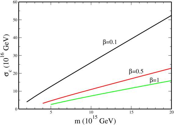
Figure 1: The critical value $\sigma_{c}$ of the inflaton field as a function of the mass parameter $m$ for $\kappa=\lambda=3\times 10^{-3}$ and $\beta=0.1$, $0.5$ and $1$, as indicated on the curves.

In figure 1, we present the critical value $\sigma_{c}$ of the inflaton field, defined in Eq.(10), as a function of the mass scale $m$ for $\kappa=\lambda=3\times 10^{-3}$ and $\beta=0.1$, $0.5$ and $1$. As can be seen from this figure, the smallest values of $\sigma_{c}$ correspond to $\beta=1$. However, in this case, the mass scale $m$ has to be $\gtrsim 5\times 10^{15}~{}{\rm GeV}$ to avoid complex values of $M$. The value of the inflaton field $\sigma_{f}$ at which inflation terminates cannot be smaller than its critical value $\sigma_{c}$ where the ‘shifted’ path becomes unstable anyway. Thus, in order to reduce the effect of SUGRA corrections which could spoil [5, 26] the flatness of the inflationary path, one would be tempted to choose values for the parameters which minimize $\sigma_{c}$. A possible set of such values is $m=5\times 10^{15}~{}{\rm GeV}$, $\kappa=\lambda=3\times 10^{-3}$ and $\beta=1$, which yield $\sigma_{c}\simeq 4\times 10^{16}~{}{\rm GeV}$. However, in this case, the condition $|\eta|=1$ implies that inflation ends at $\sigma_{f}\simeq 1.5\times 10^{18}~{}{\rm GeV}$, which is quite large. Moreover, we find that $\sigma_{Q}\simeq 1.6\times 10^{19}~{}{\rm GeV}$, which is much bigger than $m_{P}$ and, thus, this case is unacceptable.

A better set of values is $m=2\times 10^{15}~{}{\rm GeV}$, $\kappa=\lambda=5\times 10^{-3}$ and $\beta=0.1$, which also yield $\sigma_{c}\simeq 4\times 10^{16}~{}{\rm GeV}$. In this case, $\sigma_{f}\simeq 1.7\times 10^{17}~{}{\rm GeV}$ and $\sigma_{Q}\simeq 1.6\times 10^{18}~{}{\rm GeV}$, which are much smaller but still close to $m_{P}$. Values of $\beta$ smaller than $0.1$ (with suitable values of the other parameters) give also very similar results. Actually, we find that a general feature of our new shifted hybrid inflationary model is that the relevant part of inflation occurs at large values of $\sigma$ which are close to $m_{P}$. (Note that this property does not depend on the value of $(\delta T/T)_{Q}$.) Consequently, we are obliged to consider the SUGRA corrections to the scalar potential and invoke some mechanism to ensure that the ‘shifted’ inflationary path remains flat. We will address this issue in the next section.

We will now turn to the discussion of the constraints imposed on the parameter space by the measurements of the cosmic background explorer (COBE) on the quadrupole anisotropy $(\delta T/T)_{Q}$ of the CMBR . The $95\%$ confidence level allowed range of $(\delta T/T)_{Q}$, under the condition that the spectral index $n=1$, is given by [27]

$$5.4\times 10^{-6}\lesssim\left(\frac{\delta T}{T}\right)_{Q}\lesssim 7.8\times 10^{-6}.$$ (36)

The quadrupole anisotropy can be calculated as follows (see e.g., Ref.[3]):

$$\left(\frac{\delta T}{T}\right)_{Q}\simeq\frac{1}{12\sqrt{5}}\frac{V_{0}^{\frac{3}{2}}}{V^{\prime}(\sigma_{Q})m_{P}^{3}}\cdot$$ (37)

For a fixed $(\delta T/T)_{Q}$ in the range in Eq.(36), we can determine one of the free parameters (say $\beta$) in terms of the others ($m$, $\kappa$ and $\lambda$). For instance, $(\delta T/T)_{Q}\simeq 6.6\times 10^{-6}$ corresponds to $\beta=0.1$ if $m=4.35\times 10^{15}~{}{\rm GeV}$ and $\kappa=\lambda=3\times 10^{-2}$. In this case, $\sigma_{c}\simeq 3.55\times 10^{16}~{}{\rm GeV}$, $\sigma_{f}\simeq 1.7\times 10^{17}~{}{\rm GeV}$ and $\sigma_{Q}\simeq 1.6\times 10^{18}~{}{\rm GeV}$. Also, $M\simeq 2.66\times 10^{16}~{}{\rm GeV}$, $N_{Q}\simeq 57.7$ and $n\simeq 0.98$. We see that the COBE constraint can be easily satisfied with natural values of the parameters. Moreover, superheavy SM non-singlets with masses $\ll M_{GUT}$, which could disturb the unification of the SM gauge couplings, are not encountered.

3 Supergravity corrections

As we emphasized, the new shifted hybrid inflation occurs at values of $\sigma$ which are quite close to the ‘reduced’ Planck scale. Thus, one cannot ignore the SUGRA corrections to the scalar potential. The scalar potential in SUGRA, without the D-terms, is given by

$$V=e^{K/m_{P}^{2}}\left[(F_{i})^{*}K^{i^{*}j}F_{j}-3\frac{|W|^{2}}{m_{P}^{2}}\right],$$ (38)

where $K$ is the Kähler potential, $F_{i}=W_{i}+K_{i}W/m_{P}^{2}$, a subscript $i$ ($i^{*}$) denotes derivation with respect to the complex scalar field $\phi^{i}$ ($\phi^{i}\,{}^{*}$) and $K^{i^{*}j}$ is the inverse of the matrix $K_{ji^{*}}$.

Consider a (complex) inflaton $\Sigma$ corresponding to a flat direction of global SUSY with $W_{i\Sigma}=0$. We assume that the potential on this path depends only on $|\Sigma|$, which holds in our model due to a global symmetry. From Eq.(38), we find that the SUGRA corrections lift the flatness of the $\Sigma$ direction by generating a mass squared for $\Sigma$ (see e.g., Ref.[28])

$$m_{\Sigma}^{2}=\frac{V_{0}}{m_{P}^{2}}-\frac{|W_{\Sigma}|^{2}}{m_{P}^{2}}+\sum_{i,j}(W_{i})^{*}K^{i^{*}j}_{\Sigma^{*}\Sigma}W_{j}+\cdots,$$ (39)

where the right hand side (RHS) is evaluated on the flat direction with the explicitly displayed terms taken at $\Sigma=0$. The ellipsis represents higher order terms which are suppressed by powers of $|\Sigma|/m_{P}$. The slow roll parameter $\eta$ then becomes

$$\eta=1-\frac{|W_{\Sigma}|^{2}}{V_{0}}+\frac{m_{P}^{2}}{V_{0}}\sum_{i,j}(W_{i})^{*}K^{i^{*}j}_{\Sigma^{*}\Sigma}W_{j}+\cdots,$$ (40)

which, in general, could be of order unity and, thus, invalidate [5, 26] inflation. This is the well-known $\eta$ problem of inflation in local SUSY. Several proposals have been made in the literature to overcome this difficulty (for a review see e.g., Ref.[28]).

In standard and shifted SUSY hybrid inflation, there is an automatic mutual cancellation between the first two terms in the RHS of Eq.(40). This is due to the fact that $W_{n}=0$ on the inflationary path for all field directions $n$ which are perpendicular to this path, which implies that $|W_{\Sigma}|^{2}=V_{0}$ on the path. This is an important feature of these models since, in general, the sum of the first two terms in the RHS of Eq.(40) is positive and of order unity, thereby ruining inflation. It is easily checked that these properties persist in our new shifted hybrid inflationary model too. In particular, the superpotential on the ‘shifted’ inflationary path of this model takes the form $W=V_{0}^{1/2}\Sigma$.

In all these hybrid inflationary models, the only non-zero contribution from the sum which appears in the RHS of Eq.(40) originates from the term with $i=j=\Sigma$ (recall that $W_{n}=0$ on the path). This contribution is equal to the dimensionless coefficient of the quartic term $|\Sigma|^{4}/4m_{P}^{2}$ in the Kähler potential $K$. For inflation to remain intact, we need to assume [29] that this coefficient is somewhat small. The remaining terms give negligible contributions to $\eta$ provided $|\Sigma|\ll m_{P}$. The latter is true for standard and shifted hybrid inflation. So, we see that, in these models, a mild tuning of just one parameter is [29] adequate for protecting inflation from SUGRA corrections.

In our present model, however, inflation takes place at values of $|\Sigma|$ close to $m_{P}$. So, the terms in the ellipsis in the RHS of Eq.(40) cannot be ignored and may easily invalidate inflation. We, thus, need to invoke here a mechanism which can ensure that the SUGRA corrections do not lift the flatness of the inflationary path to all orders. A suitable scheme has been suggested in Ref.[23]. It has been argued that special forms of the Kähler potential can lead to the cancellation of the SUGRA corrections which spoil slow roll inflation to all orders. In particular, a specific form of $K(\Sigma)$ (used in no-scale SUGRA models) was employed and a gauge singlet field $Z$ with a similar $K(Z)$ was introduced. It was pointed out that, by assuming a superheavy VEV for the $Z$ field through D-terms, an exact cancellation of the inflaton mass on the inflationary trajectory can be achieved.

The mechanism of Ref.[23] can be readily incorporated in our model to ensure that the SUGRA corrections do not lift the flatness of the inflationary path. The only alteration caused to the Lagrangian along this path is that the kinetic term of $\sigma$ is now non-minimal. This affects the equation of motion of $\sigma$ and, consequently, the slow roll conditions, $(\delta T/T)_{Q}$ and $N_{Q}$. The form of the Kähler potential for $\Sigma$ used in Ref.[23] is given by

$$K(|\Sigma|^{2})=-Nm_{P}^{2}\ln\left(1-\frac{|\Sigma|^{2}}{Nm_{P}^{2}}\right),$$ (41)

where $N=1$ or $2$. Here we take $N=2$. In this case, the kinetic term of the real normalized inflaton field $\sigma$ (recall that $|\Sigma|=\sigma/\sqrt{2}$) is $(1/2)(\partial^{2}K/\partial\Sigma\partial\Sigma^{*})\dot{\sigma}^{2}$, where the overdot denotes derivation with respect to the cosmic time $t$ and $\partial^{2}K/\partial\Sigma\partial\Sigma^{*}=(1-\sigma^{2}/2Nm_{P}^{2})^{-2}$. Thus, the Lagrangian on the ‘shifted’ path is given by

$$L=\int_{-\infty}^{\infty}dt\int d^{3}x~{}a^{3}(t)\left[\frac{1}{2}\dot{\sigma}^{2}\left(1-\frac{\sigma^{2}}{2Nm_{P}^{2}}\right)^{-2}-V(\sigma)\right],$$ (42)

where $a(t)$ is the scale factor of the universe.

The evolution equation of $\sigma$ is found by varying this Lagrangian with respect to $\sigma$:

$$\left[\ddot{\sigma}+3H\dot{\sigma}+\dot{\sigma}^{2}\left(1-\frac{\sigma^{2}}{2Nm_{P}^{2}}\right)^{-1}\frac{\sigma}{Nm_{P}^{2}}\right]\left(1-\frac{\sigma^{2}}{2Nm_{P}^{2}}\right)^{-2}+V^{\prime}(\sigma)=0,$$ (43)

where $H$ is the Hubble parameter. During inflation, the ‘friction’ term $3H\dot{\sigma}$ dominates over the other two terms in the brackets in Eq.(43). Thus, this equation reduces to the ‘modified’ inflationary equation

$$\dot{\sigma}=-\frac{V^{\prime}(\sigma)}{3H}\left(1-\frac{\sigma^{2}}{2Nm_{P}^{2}}\right)^{2}.$$ (44)

Note that, for $\sigma\ll\sqrt{2N}m_{P}$, this equation reduces to the standard inflationary equation.

To derive the slow roll conditions, we evaluate the sum of the first and the third term in the brackets in Eq.(43) by using Eq.(44):

$$\ddot{\sigma}+\dot{\sigma}^{2}\left(1-\frac{\sigma^{2}}{2Nm_{P}^{2}}\right)^{-1}\frac{\sigma}{Nm_{P}^{2}}=\frac{V^{\prime}(\sigma)}{3H^{2}}H^{\prime}(\sigma)\dot{\sigma}\left(1-\frac{\sigma^{2}}{2Nm_{P}^{2}}\right)^{2}$$

$$-\frac{V^{\prime\prime}(\sigma)}{3H}\dot{\sigma}\left(1-\frac{\sigma^{2}}{2Nm_{P}^{2}}\right)^{2}+\frac{V^{\prime}(\sigma)}{3H}\dot{\sigma}\left(1-\frac{\sigma^{2}}{2Nm_{P}^{2}}\right)\frac{\sigma}{Nm_{P}^{2}}\cdot~{}~{}$$ (45)

Comparing the first two terms in the RHS of Eq.(45) with $H\dot{\sigma}$, we obtain

$$\epsilon\simeq\frac{1}{2}m_{P}^{2}\left(\frac{V^{\prime}(\sigma)}{V_{0}}\right)^{2}\left(1-\frac{\sigma^{2}}{2Nm_{P}^{2}}\right)^{2}\leq 1,$$ (46)

$$|\eta|\simeq m_{P}^{2}\bigg{|}\frac{V^{\prime\prime}(\sigma)}{V_{0}}\bigg{|}\left(1-\frac{\sigma^{2}}{2Nm_{P}^{2}}\right)^{2}\leq 1.~{}~{}~{}$$ (47)

The third term in the RHS of Eq.(45), compared to $H\dot{\sigma}$, yields $\sqrt{2}\sigma\epsilon^{1/2}/Nm_{P}\leq 1$, which is automatically satisfied provided that Eq.(46) holds and $\sigma\leq Nm_{P}/\sqrt{2}$. The latter is true for the values of $\sigma$ which are relevant here. We see that the slow roll parameters $\epsilon$ and $\eta$ now carry an extra factor $(1-\sigma^{2}/2Nm_{P}^{2})^{2}\leq 1$. This leads, in general, to smaller $\sigma_{f}$’s. However, in our case, $\sigma_{f}\ll\sqrt{2N}m_{P}$ (for $N=2$) and, thus, this factor is practically equal to unity. Consequently, its influence on $\sigma_{f}$ is negligible.

The formulas for $N_{Q}$ and $(\delta T/T)_{Q}$ are now also modified due to the presence of the extra factor $(1-\sigma^{2}/2Nm_{P}^{2})^{2}$ in Eq.(44). In particular, a factor $(1-\sigma^{2}/2Nm_{P}^{2})^{-2}$ must be included in the integrand in the RHS of Eq.(34) and a factor $(1-\sigma_{Q}^{2}/2Nm_{P}^{2})^{-4}$ in the RHS of Eq.(37). We find that, for the $\sigma$’s under consideration, these modifications have only a small influence on $\sigma_{Q}$ if we use the same input values for the free parameters as in the global SUSY case. On the contrary, $(\delta T/T)_{Q}$ increases considerably. However, we can easily readjust the parameters so that the COBE requirements are again met. For instance, $(\delta T/T)_{Q}\simeq 6.6\times 10^{-6}$ is now obtained with $m=3.8\times 10^{15}~{}{\rm GeV}$ keeping $\kappa=\lambda=3\times 10^{-2}$, $\beta=0.1$ as in global SUSY. In this case, $\sigma_{c}\simeq 2.7\times 10^{16}~{}{\rm GeV}$, $\sigma_{f}\simeq 1.8\times 10^{17}~{}{\rm GeV}$ and $\sigma_{Q}\simeq 1.6\times 10^{18}~{}{\rm GeV}$. Also, $M\simeq 2.6\times 10^{16}~{}{\rm GeV}$, $N_{Q}\simeq 57.5$ and $n\simeq 0.99$.

4 Conclusions

We considered the extended SUSY PS model which has been studied in Ref.[20]. This model naturally leads to a moderate violation of the ‘asymptotic’ Yukawa coupling unification so that, for $\mu>0$, the predicted $b$-quark mass can take acceptable values even with universal boundary conditions. It is [20] also compatible with all the other available phenomenological and cosmological requirements. The model contains two new superfields in the (15,2,2) representation of $G_{PS}$. The electroweak doublets in one of them mix with the electroweak doublets in the usual Higgs representation (1,2,2), thereby violating Yukawa unification. Also, the presence of two extra superfields $\phi$, $\bar{\phi}$ in the (15,1,3) representation is necessitated by the requirement that the violation of Yukawa unification is adequate.

We studied hybrid inflation within this model. The inflationary superpotential contains only renormalizable terms. In particular, the fields $\phi$, $\bar{\phi}$ lead to three new renormalizable terms which are added to the standard (renormalizable) superpotential for hybrid inflation. We showed that the resulting potential possesses a ‘shifted’ classically flat direction which can serve as inflationary path. We analyzed the spectrum of the model on this path and constructed the one-loop radiative corrections to the potential. These corrections generate a slope along this path which can drive the system towards the SUSY vacuum.

We find that the COBE constraint on the quadrupole anisotropy of the CMBR can be easily satisfied with natural values of the relevant parameters of the model. The slow roll conditions are violated well before the instability point of the ‘shifted’ path is reached and, thus, inflation terminates smoothly. The system then quickly approaches the critical point and, after reaching it, enters into a ‘waterfall’ regime during which it falls towards the SUSY vacuum and oscillates about it. Note that $G_{PS}$ is broken to $G_{S}$ already on the ‘shifted’ path and, thus, there is no monopole production at the ‘waterfall’.

As it turns out, the relevant part of inflation occurs at values of the inflaton field which are quite close to the ‘reduced’ Planck scale. We, thus, cannot ignore the SUGRA corrections which can easily invalidate inflation by generating an inflaton mass of the order of the Hubble constant. To avoid this disaster, we employ the mechanism of Ref.[23] which leads to an exact cancellation of the inflaton mass on the inflationary path. This mechanism relies on a specific Kähler potential and an extra gauge singlet with a superheavy VEV via D-terms. We show that this mechanism readily applies to our case. The COBE constraint can again be met by readjusting the input values of the free parameters which were obtained with global SUSY.