$t$-channel unitarity and photon cross sections

Abstract

We analyse the consequences of $t$-channel unitarity for the photon hadronic cross sections. We show that $\gamma^{(*)}p$ and $\gamma^{(*)}\gamma^{(*)}$ elastic amplitudes must include the complex-$j$ plane singularities associated with hadronic elastic amplitudes, and give the characteristics of possible new singularities. We also show that several different models of hadronic total cross sections can be used to predict the LEP data from the HERA measurements.

, , and

1 Introduction

The DIS and total cross section data [1, 2, 3] from HERA have opened new avenues in our understanding of strong interactions, and models [5, 6, 7] now exist which provide a unified description of $\gamma p$ interactions for photon virtualities ranging from $Q^{2}=0$ to $Q^{2}=30000$ GeV². The theoretical situation is nevertheless not clear.

Indeed, a wide range of data can be described [8, 9, 10] for $Q^{2}\geq 2$ GeV² by the DGLAP evolution [11]. Several theoretical questions need however to be addressed in this context. Firstly, the evolution is leading twist, and hence one should remove higher-twist contributions from the data before one uses the DGLAP equation. Secondly, the evolution introduces extra singularities in the complex-$j$ plane at $j=1$. These singularities start to appear at the arbitrary factorisation scale $Q_{0}$, and their re-summation leads to an essential singularity. No trace of it is however present in soft cross sections. Finally, DGLAP [11] evolution should be replaced at small $x$ by the BFKL re-summation [12]. The latter does not lead to an essential singularity in the complex-$j$ plane, but unfortunately it does not seem to be stable against next-to-leading order corrections [13].

Given these problems, Donnachie and Landshoff have proposed to use the soft pomeron as a higher-twist background to be subtracted from the evolution, while a new simple pole, the “hard pomeron”[4], would reproduce the DIS data. Furthermore, they have shown [5] that this new singularity evolves according to DGLAP, provided that one removes the $j$-plane singularities induced by DGLAP evolution, and keeps only their effect on the hard pomeron residue. Again the question arises whether such a new pole should be present in total cross sections and whether it is perturbative or not [14].

Finally, we have shown that in fact no new singularity is needed to reproduce the DIS data [6, 7], provided that one assumes a logarithmic behaviour of cross sections as functions of $\nu$. Double or triple poles at $j=1$ provide such a behaviour, and enable one to reproduce all soft and hard $\gamma p$ data within the Regge region.

How to bridge the gap between those models and QCD remains a challenge, as the description of the proton, being non-perturbative, remains at best tentative. However, LEP has now provided us with a variety of measurements of the $\gamma\gamma$ total cross sections, for on-shell photons, and of $F_{2}^{\gamma}$ for off-shell ones [15, 16]. One may hope that this will be a good testing ground for perturbative QCD [17], and that these measurements will provide guidance for the QCD understanding of existing models. Hence it is important to build a unified description of all photon processes, and to explore where perturbative effects may manifest themselves. The natural framework for such a program is the “factorisation theorem” of the analytic $S$ matrix, which relates $\gamma\gamma$, $\gamma p$ and $pp$ amplitudes. This theorem is based on $t$-channel unitarity, i.e. unitarity in the crossed channel, and in the case of simple poles one obtains the factorisation of the residues at each pole. For more general analytic structures, one obtains more complicated relations, which we shall spell out in Section 2.

Furthermore, a relation between $\gamma\gamma$ and $\gamma p$ processes may be of practical use as some of the measurements have big systematic uncertainties. As it is now well known [18], the LEP measurements are sensitive to the theoretical Monte Carlo used to unfold the data, leading to rather different conclusions concerning the energy dependence of the data. This problem is manifest in the case of total cross sections, where the unfolding constitutes the main uncertainty. In the case of HERA data, the measurement of the total cross section also seems to be affected by large uncertainties. Again, a joint study of both processes could help constrain the possible behaviours of these cross sections.

To decide whether new singularities can appear in $\gamma p$ and $\gamma\gamma$ scattering, one must first recall why singularities are supposed to be universal in hadronic cross sections. The original argument [19, 20], which we review in Section 2, used analytic continuation of amplitudes in the complex-$j$ plane from one side of a 2-particle threshold to the other, and considered only the case of simple poles. It leads to the conclusion that these poles must be universal, and that their residues must factorise.

We show in section 2 that one can generalise this formula for complex-$j$ plane amplitudes, and obtain a formulation which is valid no matter what the singularity is, and which leads to consequences similar to factorisation. Indeed, the original conclusion that singularities had to be simple poles was obtained for reggeons having resonances on their trajectories. The pomeron case may be more complicated. For instance, it is possible that no resonances are present if the real part of the trajectory never reaches integer values because of non linearity. It is also possible to imagine situations with harder singularities, such as double or triple poles, or models involving simple poles colliding at $t=0$. We want to stress here that our goal is not to decide theoretically between these possibilities by solving the unitarity equations, but only to provide a relation between various amplitudes.

We show in the third section that such a formula may be extended to photon cross sections for any value of $Q^{2}$, but that new singularities may be present in photon cross sections. If we assume as in [6, 7] that no other singularity is present in DIS, stringent constraints come from the positivity requirement for $\gamma\gamma$ total cross sections and $F_{2}$. We show that it is possible to obtain a good fit to all photon data for $Q^{2}<150$ GeV² by using either double- or triple-pole parametrisations. For total cross sections, no extra singularity seems to be needed, whereas we must introduce the singularities associated with the box diagram at high $Q^{2}$. We conclude this study by outlining its consequences on the evolution of parton distributions and on the possibility of observing the BFKL pomeron.

2 $\bf t$-channel unitarity in the hadronic case

2.1 Elastic unitarity

We start by considering the amplitudes for three related processes:

We shall refer to the momenta of the incoming particles as $p$ and $q$, and to the outgoing momentum of $a$ as $p^{\prime}$. We use the Mandelstam variables $s=(p+q)^{2}$ and $t=(p-p^{\prime})^{2}$. In the $s$ channel, these diagrams describe the processes $aa\rightarrow aa$, $ab\rightarrow ab$, and $bb\rightarrow bb$. The continuation of these amplitudes to the $t$ channel describes the processes $a\overline{a}\rightarrow a\overline{a}$, $a\overline{a}\rightarrow b\overline{b}$, $b\overline{b}\rightarrow b\overline{b}$.

We shall write $A_{ab}(l,t,m_{a},m_{b})$ for the $t$-channel partial-wave elastic amplitude for the process $a+b\rightarrow a+b$, and denote by the superscript $(1)$ the physical-sheet amplitude, and by the superscript $(2)$ its analytic continuation round a $c\bar{c}$ threshold branch point and back to the same value of $t$ (see Fig. 1).

Figure 1: The amplitude and its continuation in the complex-$t$ plane around a $c\bar{c}$ threshold.

Unitarity and analyticity of the amplitude then impose the following relation on the discontinuity through the threshold [21] :

$$A^{(1)}_{ab}-A^{(2)}_{ab}=\rho_{c}(t)A^{(1)}_{ac}A_{cb}^{(2)}=\rho_{c}(t)A^{(2)}_{ac}A_{cb}^{(1)}$$ (1)

with $\rho_{c}(t)=\sqrt{{t-4m_{c}^{2}}\over t}$.

In the case of hadrons, this leads to a closed system of equations, as the initial and final states contribute themselves to the thresholds. For instance, we can consider three coupled equations for protons and pions, across the $\pi\pi$ threshold (see Fig. 2):

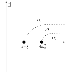
Figure 2: The amplitude and its continuation around the $\pi\pi$ and $pp$ branch-points.

$$A^{(1)}_{pp}-A^{(2)}_{pp} = \rho_{\pi}(t)A^{(1)}_{p\pi}A_{\pi p}^{(2)},$$

$$A^{(1)}_{p\pi}-A^{(2)}_{p\pi} = \rho_{\pi}(t)A^{(2)}_{p\pi}A_{\pi\pi}^{(1)},$$ (2)

$$A^{(1)}_{\pi\pi}-A^{(2)}_{\pi\pi} = \rho_{\pi}(t)A^{(1)}_{\pi\pi}A_{\pi\pi}^{(2)}.$$

From (2.1), we can write

$$A^{(1)}_{\pi\pi}=\frac{A^{(2)}_{\pi\pi}}{1-\rho_{\pi}(t)A^{(2)}_{\pi\pi}}.$$ (3)

We see that if $A^{(1)}_{\pi\pi}$ has a singularity at $j=\alpha(t)$, then $A^{(2)}_{\pi\pi}$ cannot have that singularity, which must be shifted at some other value when one goes around the cut. For instance, near a simple pole at $j=\alpha$, one has $A^{(1)}\approx{K\over j-\alpha}$, and $A^{(2)}\approx{K\over j-\alpha+\rho_{\pi}K}$.

Equation (2.1) can be conveniently written in matrix form:

$$T^{(1)}-T^{(2)}=T^{(1)}{R_{\pi}}T^{(2)}$$ (4)

with

$$T^{(i)}=\left(\begin{array}[]{cc}A^{(i)}_{\pi\pi}&A^{(i)}_{\pi p}\\ A^{(i)}_{p\pi}&A^{(i)}_{pp}\end{array}\right)\quad{\rm for}\ i=1,2$$ (5)

and the threshold matrix

$$R_{\pi}=\left(\begin{array}[]{cc}\rho_{\pi}&0\\ 0&0\end{array}\right).$$

To obtain the most constraining set of equations, one then writes the discontinuities of $A^{(2)}$ across the $pp$ threshold (the amplitudes across this threshold are denoted by a superscript (3) and $T^{(3)}$ is defined according to (5) with $i=3$). This gives, using the same notations as before:

$$T^{(2)}-T^{(3)}=T^{(2)}R_{p}T^{(3)}$$ (6)

with

$$R_{p}=\left(\begin{array}[]{cc}0&0\\ 0&\rho_{p}\end{array}\right).$$

Putting Eqs. (4, 6) together, one then gets:

$$T^{(1)}-T^{(3)} = T^{(1)}R_{\pi}T^{(2)}+T^{(2)}R_{p}T^{(3)}$$ (7)

$$= T^{(1)}(R_{\pi}+R_{p})T^{(3)}+T^{(1)}R_{\pi}(T^{(2)}-T^{(3)})$$

$$\phantom{T^{(1)}(R_{\pi}+R_{p})T^{(3)}}+(T^{(2)}-T^{(1)})R_{p}T^{(3)}$$

$$= T^{(1)}RT^{(3)}$$

with $R=R_{\pi}+R_{p}$. Note that $T^{(3)}={T^{(1)}}^{\dagger}$.

One can then solve the equation for $T^{(1)}$ to obtain

$$T^{(1)}\left[1-RD\right]=D$$ (8)

with $D={T^{(1)}}^{\dagger}$. This situation generalises that of Eq. (3): $T^{(1)}$ is a function of ${T^{(1)}}^{\dagger}$ and its singularities cannot come from singularities in the right-hand side of Eq. (8), because they are exactly matched by corresponding factors in the left-hand side. Note that this is why we needed to consider both thresholds, as otherwise some amplitudes would not be present in the r.h.s. of (7).

Hence the amplitudes $A^{(1)}_{\pi\pi}$, $A^{(1)}_{pp}$ and $A^{(1)}_{\pi p}$ have common singularities which can only come from zeroes $z_{m}$ of the determinant of the matrix in brackets in the left-hand side of (8):

$$\Delta=\det\left(1-RD\right)=0\;{\rm for}\;j=z_{m},\ m=1,...,N.$$ (9)

The determinant can then be written

$$\Delta=\prod\limits_{m=1}^{N}\Delta_{m}$$ (10)

with $\Delta_{m}=0$ at $j=z_{m}$ and $\Delta_{m}\neq 0$ at $j=z_{k}$ if $k\neq m$. $A^{(1)}_{il}$ (where $i$ and $l$ stand for $p$ or $\pi$) then becomes

$$A^{(1)}_{il}=\sum_{m=1}^{N}\left({a_{il;\,m}\over\Delta_{m}}\right)+F_{il}$$ (11)

where $F_{il}$ and $a_{il;\,m}$ are functions of $j$ finite at each $z_{m}$.

This is the basis of the complex-$j$-plane factorisation of the amplitudes contained in $T^{(1)}$. Indeed, we can write

$$A^{(1)}_{pp}A^{(1)}_{\pi\pi}-\left(A^{(1)}_{\pi p}\right)^{2}=\det(T^{(1)})=\frac{\det(D)}{\Delta}.$$ (12)

Multiplying both sides of (12) by $\Delta_{k}^{2}$, and using (11), this gives

$$\left\{\left[a_{pp;\,k}+\Delta_{k}\sum_{m\neq k}\left({a_{pp;\,m}\over\Delta_{m}}\right)+\Delta_{k}F_{pp}\right]\left[a_{\pi\pi;\,k}+\Delta_{k}\sum_{m\neq k}\left({a_{\pi\pi;\,m}\over\Delta_{m}}\right)+\Delta_{k}F_{\pi\pi}\right]\right.$$

$$-\left.\left[a_{\pi p;\,k}+\Delta_{k}\sum_{m\neq k}\left({a_{\pi p;\,m}\over\Delta_{m}}\right)+\Delta_{k}F_{\pi p}\right]\left[a_{\pi p;\,k}+\Delta_{k}\sum_{m\neq k}\left({a_{\pi p;\,m}\over\Delta_{m}}\right)+\Delta_{k}F_{\pi p}\right]\right\}$$ (13)

$$= \Delta_{k}\left\{{\det(D)\over\Delta_{1}...\Delta_{k-1}\Delta_{k+1}...\Delta_{N}}\right\}$$

In the limit $j\rightarrow z_{k}$, $\Delta_{k}\rightarrow 0$, and we get

$$a_{pp;\,k}\ a_{\pi\pi;\,k}-\left(a_{\pi p;\,k}\right)^{2}=0\quad{\rm for}\ k=1,...,N$$ (14)

or equivalently

$$\lim_{j\rightarrow z_{k}}\left[A^{(1)}_{pp}(j)-\frac{\left(A^{(1)}_{\pi p}(j)\right)^{2}}{A^{(1)}_{\pi\pi}(j)}\right]=\rm finite\>terms.$$ (15)

The relations (8) and (12) hold for all values of $t$ above the $4m_{p}^{2}$ threshold. Hence they must hold for all $t$ as the amplitudes are analytic, and in particular they can be continued to negative $t$. The consequence (14) must thus remain true for the amplitude in the direct channel.

We show in Appendix 1 that this relation remains the same in the case of an arbitrary number of elastic and inelastic thresholds:

$$T^{(1)}({1\rm I}-RD)=D$$ (16)

where $T^{(1)}$ is the matrix containing all elastic amplitudes, and $D$ is now an unknown matrix containing the effects of inelastic thresholds and the contribution of elastic amplitudes across the cuts. Again, the singularities of $T^{(1)}$ must come from the zeroes $z_{m}$ of

$$\Delta=\det({1\rm I}-RD)$$ (17)

and one obtains again (14) and (15).

2.2 Properties

1. The factorisation relations are in general broken when one calculates the contribution of multiple exchanges of trajectories. However, as the above argument is totally general, after all the ($s$-channel) unitarising exchanges are taken into account, one must end up again with an amplitude factorising at each singularity, even if the latter is not a simple pole.

2. The matrix $D$ is sensitive to the existence of thresholds associated with bound states, and does not know directly about quarks and gluons which do not enter the unitarity equations. Hence the zeroes $z_{m}$ are not calculable perturbatively.

3. One could have a spurious cancellation of the singularity if some element of $D$ has a zero at $j=z_{m}$. However, it is unlikely for this cancellation to occur for all $t$ or for all processes. It is however possible to “hide” a singularity, e.g. at $t=0$ for $pp$ and $\bar{p}p$ scattering. This might provide an explanation for the absence of an odderon pole in forward scattering data.

4. Each singularity factorises separately. Hence it does not make sense to consider globally factorising cross sections or amplitudes in the $s$, $t$ representation, unless of course the amplitude can be reproduced by only one leading singularity.

5. The relations (15) lead to a definite prediction for the residues (or couplings) of the singularities above threshold $t>4m_{a}^{2}$. As no singularity occurs when $t$ is continued to the physical region for the $s$ channel processes, these relations remain true there.

6. We have mentioned that one always obtains a relation between the amplitude and its complex conjugate. In fact, this is derived in Appendix 1 as a consequence of the unitarity of the $S$ matrix. The relations between amplitudes across a cut are really derived from the relation between the amplitude and its complex conjugate, and hold for whatever structure the cuts have.

2.3 Specific examples

Eq. (15) is usually not mentioned, and only its consequences for the residues of simple poles are considered. However, we have shown that it is true in general, and that leads to specific predictions for any singularity structure of the amplitudes $A^{(1)}_{il}(j)$, e.g. for a given order of the zeroes $z_{m}$. We shall give here the formulae that correspond to simple, double or triple poles, which seem to be three possibilities emerging from fits to hadronic amplitudes at $t=0$ [23]. We shall refer to these relations as the $t$-Channel Unitarity relations. The case of cuts will not be explicitly considered here, although Eq. (15) holds also in this case.

For isolated simple poles

$$A^{(1)}_{il}=\sum_{m}\frac{R_{il;\,m}}{j-z_{m}},$$ (18)

one obtains the usual relations for the residues [19]

$$R_{22;\,m}=\frac{\left(R_{12;\,m}\right)^{2}}{R_{11;\,m}}.$$ (19)

If $A^{(1)}_{il}$ has coinciding simple and double poles

$$A^{(1)}_{il}=\frac{S_{il}}{j-z}+\frac{D_{il}}{(j-z)^{2}},$$ (20)

one obtains the new relations

$$D_{11}D_{22} = {\left(D_{12}\right)^{2}},$$

$$D_{11}S_{22}+S_{11}D_{22} = {2D_{12}S_{12}}.$$ (21)

In the case of triple poles

$$A^{(1)}_{il}=\frac{S_{il}}{j-z}+\frac{D_{il}}{(j-z)^{2}}+\frac{F_{il}}{(j-z)^{3}},$$ (22)

the relations become

$$F_{11}F_{22} = {\left(F_{12}\right)^{2}},$$

$$F_{11}D_{22}+D_{11}F_{22} = {2F_{12}D_{12}},$$ (23)

$$D_{11}D_{22}+S_{11}F_{22}+S_{22}F_{11} = 2S_{12}F_{12}+D_{12}^{2}.$$

It is worth pointing out that the double-pole relations are not the limit of the triple-pole relations for a vanishing triple-pole residue. Similarly, the simple-pole relations cannot be obtained from the double-pole ones. The reason for this is that the relations (12) relate the poles of order $2n$ to $n+1$, $n$ being the maximal order of the pole. Hence the first double-pole relation is contained in the triple-pole ones, but not the second one, and the simple-pole relations are entirely separate.

3 The photon case

Photons can also be considered within the formalism of $t$-channel unitarity. However, it is unclear whether the elastic cross section can be measured, or even defined [24]. In practise, what is measured is the hadronic part of the cross section. Hence only the hadronic part of the photon wave function enters the measurement, and this part is not directly related to the $S$ matrix.

The way to circumvent this problem is to consider the photons as external state insertions on the hadronic $S$ matrix. This means that they will enter the unitarity equations only as external states, and will not contribute to the thresholds.

In practise, the equations (12, 16) remain the same, provided that we write the threshold matrix $R$ as

$$R=\left(\begin{array}[]{cc}\rho_{p}&0\\ 0&0\end{array}\right).$$ (24)

This means that $\Delta=1-\rho_{p}D_{pp}$ only involves $D_{pp}$, hence singularities can now come from other elements of $D$, and $\det(D)$ can contain singularities not present in $\Delta,$ hence breaking the factorisation relations (12,15). Namely, we obtain

$$A^{(1)}_{pp} = \frac{D_{pp}}{\Delta},$$

$$A^{(1)}_{\gamma p} = \frac{D_{\gamma p}}{\Delta},$$ (25)

$$A^{(1)}_{\gamma\gamma} = \frac{\rho_{p}D_{\gamma p}^{2}}{\Delta}+D_{\gamma\gamma}.$$

Extra singularities can come from $D_{\gamma p}$ or $D_{\gamma\gamma}$. In the first case, the nature of the singularity is different in $\gamma p$ and in $\gamma\gamma$, and the coupling of the singularity, which contains $\Delta$, must be of non-perturbative origin. On the other hand, singularities in $D_{\gamma\gamma}$ can be purely perturbative.

In the DIS case, the off-shell photons can also be treated as external particles, and one recovers the above equations (25) and the possibility of extra singularities. Details and general formulae are given in Appendix 2, where one obtains an equation similar to (25), with a matrix $D$ depending on the off-shellnesses of photons:

$$T^{(1)}(Q_{in},Q_{out})=D(Q_{in},Q_{out})+\frac{D(Q_{in},0)RD(0,Q_{out})}{{1\rm I}-RD(0,0)}.$$ (26)

where $Q_{in}$ stands for the two virtualities $(Q_{1}^{2},Q_{2}^{2})$ of the initial states in the $t$ channel, and $Q_{out}$ for the two virtualities $(Q_{3}^{2},Q_{4}^{2})$ of the final states.

We want to point out that the position of the possible new singularities can depend on $Q^{2}$, and as the off-shell states do not enter unitarity equations, these singularities can be fixed in $t$.

4 Test of $t$-Channel Unitarity relations

In order to test the previous equations, and to evaluate the need for new singularities, we shall use models that reproduce $pp$, $\gamma p$ and $\gamma\gamma$ cross sections. Previous studies [23] have shown that there are at least three broad classes of models that can reproduce all forward hadron and photon data.

The general form of these parametrisations is given, for total cross sections of $a$ on $b$, by the generic formula

$$\sigma^{tot}_{ab}=(R_{ab}+H_{ab})/s$$ (27)

where $R_{ab}$ is the contribution of the highest meson trajectories ($\rho$, $\omega$, $a$ and $f$) and the rising term $H_{ab}$ stands for the pomeron. The first term is parametrised via Regge theory, and we allow the lower trajectories to be partially non-degenerate, i.e. we allow one intercept for the charge-even trajectories, and another one for the charge-odd ones [27]. Hence we use

$$R_{ab}=Y_{ab}^{+}\left({\tilde{s}}\right)^{\alpha_{+}}\pm Y_{ab}^{-}\left({\tilde{s}}\right)^{\alpha_{-}}$$ (28)

with $\tilde{s}=2\nu/(1$ GeV${}^{2})$, $\nu=p.q$.

As for the pomeron term, we consider the following possibilities:

$$H_{ab} = X_{ab}\left[\widetilde{s}\right]^{\alpha_{\wp}},$$ (29)

$$H_{ab} = {\tilde{s}}D_{ab}\left[\log\widetilde{s}+\log C_{ab}\right],$$ (30)

$$H_{ab} = {\tilde{s}}t_{ab}\left[\log^{2}\left(\frac{\widetilde{s}}{d_{ab}}\right)+\log\left(c_{ab}\right)\right].$$ (31)

These forms come from simple, double or triple poles in the Watson-Sommerfeld transform of the amplitude (see Eq. (59) of Appendix 1), in the limit of $\cos(\vartheta_{t})$ large, so that the contribution from the integration contour vanishes, and that one can keep only the leading meson trajectories and the pomeron contribution.

Using the asymptotic expansion of the Legendre polynomials $P_{l}$

$$P_{l}(-\cos(\vartheta_{t}))\rightarrow\frac{\Gamma(2l+1)}{[\Gamma(l+1)]^{2}2^{l}}\left(\frac{\nu}{m_{p}^{2}}\right)^{l},$$ (32)

we obtain, by the residue theorem (see Eq. (59) of Appendix 1), the following contributions to the total cross section for simple, double, and triple poles:

$$A^{(1)}(j,0) = \frac{g}{j-\alpha}$$ (33)

$$\rightarrow \sigma_{tot}=g\left(\frac{\nu}{m_{p}^{2}}\right)^{\alpha}\frac{(2\alpha+1)\Gamma(2\alpha+1)}{(\Gamma(\alpha+1))^{2}2^{\alpha}},$$

$$A^{(1)}(j,0) = \frac{g}{(j-\alpha)^{2}}$$ (34)

$$\rightarrow \sigma_{tot}=g\left(\frac{\nu}{m_{p}^{2}}\right)^{\alpha}\log\left(\frac{\nu}{m_{p}^{2}}\right)\frac{(2\alpha+1)\Gamma(2\alpha+1)}{(\Gamma(\alpha+1))^{2}2^{\alpha}},$$

$$A^{(1)}(j,0) = \frac{g}{(j-\alpha)^{3}}$$ (35)

$$\rightarrow \sigma_{tot}=g\left(\frac{\nu}{m_{p}^{2}}\right)^{\alpha}\log^{2}\left(\frac{\nu}{m_{p}^{2}}\right)\frac{(2\alpha+1)\Gamma(2\alpha+1)}{(\Gamma(\alpha+1))^{2}2^{\alpha+1}}.$$

In the photon case, things are a little different. Looking first at the $\gamma p$ amplitude with off-shell photons, we have

$$|\cos(\vartheta_{t})|=\frac{\nu}{m_{p}\sqrt{Q^{2}}}.$$ (36)

In the on-shell limit $Q^{2}\rightarrow 0$, the Legendre polynomial of Eq. (32) becomes infinite, hence one must assume that the amplitude goes to zero in such a way that the limit is finite. One can take for instance

$$A^{(1)}_{\gamma p}=\tilde{A}^{(1)}_{\gamma p}\left(\frac{\sqrt{Q^{2}}}{q_{\gamma}(Q^{2})}\right)^{j}$$ (37)

with $q_{\gamma}(0)$ finite. Such a choice introduces a new scale that effectively replaces $\sqrt{Q^{2}}$ with $q_{\gamma}(Q^{2})$ in $\cos(\vartheta_{t})$, and $A^{(1)}$ with $\tilde{A}^{(1)}$. In the $\gamma\gamma$ case, with $Q^{2}$ and $P^{2}$ the off-shellnesses of the two incoming photons, in order to keep the unitarity relations (12) for the amplitude $\tilde{A}^{(1)}$ instead of $A^{(1)}$, one needs to assume that

$$A^{(1)}_{\gamma\gamma}=\tilde{A}^{(1)}_{\gamma\gamma}\left(\frac{\sqrt{Q^{2}P^{2}}}{q_{\gamma}(Q^{2})q_{\gamma}(P^{2})}\right)^{j}$$ (38)

and the scales $q_{\gamma}(Q^{2})$ and $q_{\gamma}(P^{2})$ replace $m_{p}$ in Eqs. (33-35).

4.1 Regge region

One can think of translating the minimum $\sqrt{s}$ of the $pp$ case into a bound for ${\nu}/{m_{p}^{2}}$, ${\nu}/({m_{p}q_{\gamma}(Q^{2})})$ and ${\nu}/{q_{\gamma}^{2}(Q^{2})}$, and use the same bound in the three processes. Unfortunately, the situation is really more complicated because one cannot extract $q_{\gamma}(Q^{2})$ from the data as the $\log\nu$ terms come from a combination of simple, double (and triple) poles at $j=1$, which can always be re-shuffled among themselves.

In the following, we shall use cuts on the natural Regge variables $2\nu$, and $\cos(\vartheta_{t})$. We find that data are well reproduced in the region

$$\cos(\vartheta_{t}) \geq \frac{49{\rm\ GeV}^{2}}{2m_{p}^{2}},$$ (39)

$$\sqrt{2\nu} \geq 7\ \rm GeV.$$ (40)

For the $\gamma\gamma$ and the $\gamma p$ total cross sections, as well as for the photon structure function where $P^{2}\rightarrow 0$, $\cos(\vartheta_{t})$ becomes infinite, and only the cut on $2\nu$ constrains the Regge region.

Furthermore, in the case of one virtual photon, experimentalists measure the $ep$ or the $e\gamma$ cross sections. From these, one can extract a cross section for $\gamma^{*}p$ or $\gamma^{*}\gamma^{*}$ scattering, provided one factors out a flux factor. As is well known, the latter is univoquely defined only for on-shell particles:

$$\sigma_{tot}=\lim_{Q^{2}\rightarrow 0}\frac{4\pi^{2}\alpha}{Q^{2}}F_{2}.$$ (41)

The flux factor can then be modified arbitrarily, provided that the modifications vanish as $Q^{2}\rightarrow 0$. This means, for instance, that we can always multiply the left-hand side of (41) by an arbitrary power of $(1-x)$. Hence one should in principle limit oneself to small values of $x$ only. We find that we can obtain good fits in the region

$$x\leq 0.3.$$ (42)

Note that in the case of two off-shell photons, experimentalists measure $\sigma_{TT}+\sigma_{TL}+\sigma_{LT}+\sigma_{LL}$, which is precisely the quantity entering the factorisation theorem. Hence no flux factor is necessary here.

Finally, all the residues are expected to be functions of $Q^{2}$. These form factors are unknown, and are expected to contain higher twists. In order to check factorisation, we do not want to be too dependent on these guesses. Hence we choose a modest region of

$$Q^{2}\leq 150\ {\rm GeV}^{2},$$ (43)

where most of the $\gamma^{*}\gamma^{*}$ points lie.

We shall consider in the next section possible extensions to a wider region.

4.2 Factorising $t$-Channel Unitarity relations

As explained above, the simple-pole singularities will factorise in the usual way. Note that there is no charge-odd singularity in the photon case, hence only the $a/f$ lower trajectory will enter the relations. One then gets

$$Y_{pp}Y_{\gamma\gamma}(P^{2},Q^{2})=Y_{\gamma p}(P^{2})Y_{\gamma p}(Q^{2}).$$ (44)

In the case of a soft-pomeron pole, one obtains similarly

$$X_{pp}X_{\gamma\gamma}(P^{2},Q^{2})=X_{\gamma p}(P^{2})X_{\gamma p}(Q^{2}).$$ (45)

The case of multiple poles is given by Eqs. (21, 23), and can be made more transparent by using the forms (30, 31) which give factorisation-looking relations for the constants (but not for all the residues! $-$ see Eqs. (21) and (23) $-$):

$$f_{pp}f_{\gamma\gamma}(P^{2},Q^{2})=f_{\gamma p}(P^{2})f_{\gamma p}(Q^{2})$$ (46)

with $f=D$, $C$, $t$, $d$ or $c$.

4.3 Dataset

For the total cross sections, we have used the updated COMPETE dataset used in [29], which is the same as that of [30] except for the inclusion of the latest ZEUS results on $\gamma p$ cross section [2] and for the inclusion of cosmic-ray data.

For $\gamma p$ scattering, we have used the full set of available data [1, 2, 28].

For the $\gamma\gamma$ measurements of $F_{2}^{\gamma}$, we have used the data of [15, 16], whenever these included the joint $x$ and $Q^{2}$ (and $P^{2}$) dependence. We have not included other data as they do not have points in the Regge region. Note that we have not taken the uncertainties in $x$ into account, hence the $\chi^{2}$ values are really upper bounds in the $\gamma\gamma$ case.

4.4 Previous parametrisations

We have first considered the results using previous studies [6, 7] of $\gamma^{(*)}p$ and $pp$ scattering. Making use of the $t$-Channel Unitarity relations (21) and (23), we have obtained reasonably good predictions for $\sigma_{\gamma\gamma}$ and $F_{2}^{\gamma}$. However, the formalism breaks down in the case of $\gamma^{*}\gamma^{*}$ scattering, because the form factors that we used do not guarantee the positivity of the charge-even part of the cross sections. Re-fitting them enables one to get closer to the data, but the problem of negativity remains in some part of the physical region. Hence, at this point, the factorisation relations have one major consequence: the parametrisations of [6, 7] are ruled out.

We have also considered the hard pomeron fit of [5] where the charge-parity $+1$ rising term contains two different simple poles: the soft and the hard pomeron. In this case, the soft pomeron residues factorise. The hard pomeron, if it is not present in $pp$ cross sections (see however [14]), then comes in as a double pole in $\gamma\gamma$ cross sections, see Eq. (25), and produces a cross section proportional to $\nu^{\alpha_{h}}\log\nu$. Its residue will then depend on the value of $\Delta(j=\alpha_{h})$, which is unknown. This means that factorisation does not say much about the hard pomeron contribution, which can always be arbitrarily re-scaled. It is possible to get good fits using these forms, but as they do not test factorisation, we shall not present these results here.

4.5 New parametrisation: triple pole

In the triple-pole case, the problem of negativity can be cured through the introduction of another functional form for the form factors. To convince ourselves that this is possible, we have fitted $F_{2}$ in several $Q^{2}$ bins to

$$F_{2}^{p}(Q^{2})=a(\log\nu+b)^{2}+c\nu^{-0.47}.$$ (47)

From the values of $a,$ $b$ and $c$, and the $t$-Channel Unitarity relations, one can then predict the symmetric $F_{2}^{\gamma}(Q^{2},Q^{2})$. The result of this exercise is shown in Fig. 3.

Figure 3: Prediction from $t$-Channel Unitarity relations for the $\gamma^{*}\gamma^{*}$ cross section, including the box diagram of Appendix 3.

One clearly sees that there are two branches in the fit to HERA data: one with positive $b$, and another one with negative $b$. Both have comparable $\chi^{2}$, but one produces positive $\gamma\gamma$ cross sections, whereas the other one does not. Armed with this information, we found that the resulting form factors could be well approximated by the following forms:

$$t_{\gamma p}(Q^{2}) = t_{1}\left(\frac{1}{1+\frac{Q^{2}}{Q_{t}^{2}}}\right)^{\epsilon_{t}},$$

$$Y^{+}_{\gamma p}(Q^{2}) = Y_{1}\left(\frac{1}{1+\frac{Q^{2}}{Q_{y}^{2}}}\right)^{\epsilon_{y}},$$ (48)

$$\log d_{\gamma p}(Q^{2}) = d_{1}\left(\frac{Q^{2}}{Q^{2}+Q_{d}^{2}}\right)^{\epsilon_{d}},$$

$$\log c_{\gamma p}(Q^{2}) = c_{0}+c_{1}\left(\frac{1}{1+\frac{Q^{2}}{Q_{c}^{2}}}\right)^{\epsilon_{c}}.$$

With the form factors obtained from our fit, we have then checked that the $\gamma^{*}\gamma^{*}$ cross section remains positive everywhere.

4.6 New parametrisation: double pole

In the case of a double pole, Fig. 3 shows that the situation is more difficult, as one cannot guarantee positivity. We have tried several possibilities, among which a further splitting of leading meson trajectories along the lines of [31], but found that positivity is still not guaranteed.

However, it is possible to obtain a good fit, positive everywhere, if one assumes a slightly modified version of the double pole [32].

Instead of taking an $\tilde{s}D\log\tilde{s}$ term in $H_{ab}$ as in Eq. (30), one can consider

$$H_{ab}=\tilde{s}D_{ab}\ [L_{ab}+\log C_{ab}]$$ (49)

with

$$L_{ab}(\tilde{s})=\frac{1}{2}\Re e[\log(1+\Lambda_{ab}\tilde{s}\,^{\delta})+\log(1+\Lambda_{ab}(-\tilde{s})\,^{\delta})].$$ (50)

Asymptotically, this gives the same form as a double pole. Furthermore, one can rewrite $\log(1+\Lambda_{ab}(\tilde{s})\,^{\delta})=\delta\log(\tilde{s})+\log(\Lambda_{ab}+1/(\tilde{s})\,^{\delta})$. The first term comes from a double pole at $j=1$, whereas the Taylor expansion of the remaining term gives a series of simple poles. Hence $D_{ab}$ and $\Lambda_{ab}$ factorises according to

$$D_{\gamma\gamma}(P^{2},Q^{2})D_{pp} = D_{\gamma p}(P^{2})D_{\gamma p}(Q^{2}),$$

$$\Lambda_{\gamma\gamma}(P^{2},Q^{2})\Lambda_{pp} = \Lambda_{\gamma p}(P^{2})\Lambda_{\gamma p}(Q^{2}).$$ (51)

We found good fits using the following form factors:

$$D_{\gamma p} = D_{1}\left(\frac{1}{1+\frac{Q^{2}}{Q_{d}^{2}}}\right)^{\epsilon_{d}},$$

$$D_{\gamma p}\log C_{\gamma p} = C_{1}\left(\frac{1}{1+\frac{Q^{2}}{Q_{c}^{2}}}\right)^{\epsilon_{c}},$$ (52)

$$\Lambda_{\gamma p} = \Lambda_{1}\left(\frac{1}{1+\frac{Q^{2}}{Q_{\lambda}^{2}}}\right)^{\epsilon_{\lambda}},$$

$$Y^{+}_{\gamma p}(Q^{2}) = Y_{1}\left(\frac{1}{1+\frac{Q^{2}}{Q_{y}^{2}}}\right)^{\epsilon_{y}}.$$

		double		triple
Quantity	$N$	$\chi^{2}$	$\chi^{2}/N$	$\chi^{2}$	$\chi^{2}/N$
$F_{2}^{p}$	821	789.624	0.962	870.599	1.060
$F_{2}^{\gamma}$	65	57.686	0.887	59.963	0.923
$\sigma_{\gamma\gamma}$	32	19.325	0.604	15.568	0.487
$\sigma_{\gamma p}$	30	17.546	0.585	21.560	0.719
$\sigma_{pp}$	90	100.373	1.115	82.849	0.921
$\sigma_{p\bar{p}}$	49	55.240	1.127	58.900	1.202
$\rho_{pp}$	67	93.948	1.402	98.545	1.471
$\rho_{p\bar{p}}$	11	16.758	1.523	4.662	0.424
Total	1165	1150.500	0.988	1212.645	1.041

Table 1: Results of fits to a generalised double pole model and to a triple pole model, using the form factors of Eqs. (48) and (52). $N$ is the number of data points for each sub-process.

4.7 Box diagram

Figure 4: The box diagram contribution.

One new singularity may be present in $\gamma\gamma$ scattering: it is the box diagram, shown in Fig. 4, which couples directly two photons to quarks. This diagram must be present when the photons are far off-shell and pQCD applies. As we have explained above, it is not at all obvious that it is present in the case of total cross sections, and in fact we get better fits if we include it only for off-shell photons. Hence an extra perturbative singularity is needed at nonzero $Q^{2}$.

We have re-calculated it and confirm the results of [33] (see Appendix 3). In the following, we shall fix the quark masses at

$$m_{u}=m_{d} = 0.3{\ \rm GeV},$$

$$m_{s} = 0.5{\ \rm GeV},$$ (53)

$$m_{c} = 1.5{\ \rm GeV},$$

$$m_{b} = 4.5{\ \rm GeV}.$$

and the quarks are included only above threshold $s=2\nu-P^{2}-Q^{2}>4m_{q}^{2}$.

4.8 Results

As we want to be able to vary the minimum value of $2\nu$, and as the fits of [23] neither include the generalised dipole nor use $2\nu$ as the energy variable, we have re-fitted the $pp$ and $\bar{p}p$ cross sections and $\rho$ parameter together with those for $\gamma^{(*)}p$ and $\gamma^{(*)}\gamma^{(*)}$, and imposed factorisation of the residues.

triple		double
Parameter	Value	Parameter	Value
$t_{pp}$	0.6264 $\pm$0.0055	$\Lambda_{pp}$	$1.36\pm 0.15$
$log(d_{pp})$	0.534 $\pm$0.044	$D_{pp}$	$40.3\pm 1.4$
$t_{pp}\log c_{pp}$	65.86 $\pm$0.48	$D_{pp}\log C_{pp}$	$-32.7\pm 5.3$
$Y^{+}_{pp}$	122.0 $\pm$ 1.5	$Y^{+}_{pp}$	$231.1\pm 4.7$
$\alpha_{+}$	0.6905$\pm$0.0023	$\alpha_{+}$	$0.7263\pm 0.0010$
$Y^{-}_{pp}$	84.6 $\pm$4.1	$Y^{-}_{pp}$	$97.6\pm 4.6$
$\alpha_{-}$	0.4596$\pm$0.0010	$\alpha_{-}$	$0.505\pm 0.015$
$c_{0}$	$-613.93\pm 0.91$	$\delta$	$0.3313\pm 0.0092$
$c_{1}$	740.8 $\pm$1.2	$C_{1}$	$-0.105\pm 0.016$
$Q^{2}_{c}$	0.1557 $\pm$0.0030	$Q^{2}_{c}$	$0.0219\pm 0.0076$
$\epsilon_{c}$	0.11619 $\pm$ 0.00047	$\epsilon_{c}$	$0.553\pm 0.025$
$t_{1}$	0.001667$\pm$0.000011	$\Lambda_{1}$	$1.49\pm 0.23$
$Q^{2}_{t}$	0.964 $\pm$ 0.016	$Q^{2}_{\lambda}$	$0.111\pm 0.032$
$\epsilon_{t}$	0.8237$\pm$ 0.0034	$\epsilon_{\lambda}$	$0.658\pm 0.019$
$d_{1}$	-8.067$\pm$0.033	$D_{1}$	$0.1305\pm 0.0062$
$Q^{2}_{d}$	7.56 $\pm$0.25	$Q^{2}_{d}$	$0.379\pm 0.061$
$\epsilon_{d}$	0.3081 $\pm$ 0.0059	$\epsilon_{d}$	$0.434\pm 0.021$
$Y_{1}$	0.1961 $\pm$0.0031	$Y_{1}$	$0.515\pm 0.017$
$Q^{2}_{y}$	2.056 $\pm$ 0.067	$Q^{2}_{y}$	$0.158\pm 0.016$
$\epsilon_{y}$	0.5448 $\pm$ 0.0049	$\epsilon_{y}$	$0.709\pm 0.016$

Table 2: Parameters (in natural units) of the global fits.

Figure 5: Fits to the total cross sections and to the $\rho$ parameters.

Figure 6: Form factors of the triple pole (left) and double pole (right) parametrisations.

We show in Table 1 the $\chi^{2}$ per data point and the number of points for each process. We see that one obtains a very good global $\chi^{2}$ for both models. It is well known [23] that the partial $\chi^{2}$ for $\sigma_{p\bar{p}}$ and $\rho_{pp}$ never reach low values, presumably because of the presence of contradictory data. We show the corresponding curves in Fig. 5.

The values of the parameters are given in Table 2 for the triple-pole and the double-pole cases, and the form factors are plotted in Fig. 6.

We see that the intercepts of the leading meson trajectories are close, in fact closer than those of [23]. This is due to the smaller energy region, and to the much larger influence of photon data on $\alpha_{+}$.

It may also be noted, in the double-pole case, that the parameter $\delta$ is close to the hard pomeron intercept of [5]. At high $Q^{2}$, because the form factor $\Lambda$ falls off, the logarithm starts looking like a power of $2\nu$, and somehow mimics a simple pole. It may thus be thought of as a unitarized version of the hard pomeron, which would in fact apply to hard and soft scatterings.

In the triple-pole case, this is accomplished by a different mechanism: the scale of the logarithm is a rapidly falling function of $Q^{2}$, and hence the $\log^{2}$ term becomes relatively more important at high $Q^{2}$. Interestingly, when one writes the triple-pole parametrisation as a function of $x$ and $Q^{2}$, one obtains only very small powers (of the order of 0.1) of $Q^{2}$, which do not contain any higher twists, contrarily to the soft pomeron of [5].

4.9 Total $\gamma p$ and $\gamma\gamma$ cross sections

We see from Table 1 that one obtains an excellent $\chi^{2}$ for $\sqrt{2\nu}>7$ GeV, for a total of 62 points. The curves are shown in Fig. 5. The fit can in fact be continued to $\sqrt{2\nu}=2$ GeV, with a $\chi^{2}$/point of 0.74 for 219 points.

We have checked that adding the box diagram leads to a slight degradation of the fit, whether one fits the total cross sections alone or with all other data. As the contribution of the box is calculated perturbatively, one might object that one cannot use the result down to $Q^{2}=0$, and that only the $\nu$ dependence should be kept. Hence we have also tried to add an extra term, proportional to $\log\nu/\nu$ in the total cross section, but found that the fit prefers to set the proportionality constant to zero. Hence it seems that this singularity is not needed at $P^{2}=Q^{2}=0$. However, because of large uncertainties in the data, it is not possible to rule it out altogether.

Similarly, we do not find the need to introduce any new rising contribution. However, it is clear in view of the large uncertainties that it is not possible to rule out completely such a possibility. In fact, our fit prefers the $\gamma\gamma$ data unfolded with PHOJET [36], which rise more slowly than those unfolded with PYTHIA [37]. Interestingly, as we reproduce both HERA and LEP data, for $Q^{2}$ nonzero, it is not true that an extrapolation of the nonzero $Q^{2}$ data leads to a higher estimate of the $\gamma p$ and $\gamma\gamma$ cross sections. Our fit can be considered as an explicit example for which such an extrapolation leads to a cross section on the lower side of the experimental errors.

Figure 7: Fits to $F_{2}^{p}$ in the high-$Q^{2}$ region. We show only graphs for which there are more than 6 experimental points.

Figure 8: Fits to $F_{2}^{p}$ in the low-$Q^{2}$ region. We show only graphs for which there are more than 6 experimental points, as well as the lowest-$Q^{2}$ ones. The curves and the data are as in Fig. 7.

4.10 $F_{2}^{p}$

The fit to $F_{2}$ has quite a good $\chi^{2}$ as well. We have checked that one can easily extend it to $Q^{2}\approx 400$ GeV² for the triple pole, and to $Q^{2}\approx 800$ GeV² in the double-pole case. It is interesting that one cannot go as high as in ref. [7]. This can be attributed either to too simple a choice for the form factors, or to the onset of perturbative evolution.

Figs. 7 and 8 show the $F_{2}^{p}$ fit for the most populated $Q^{2}$ bins. As pointed out before, we see that our fits do reproduce the low-$Q^{2}$ region quite well, but predict total cross sections on the lower side of the error bands. Hence the extrapolation to $Q^{2}=0$ of DIS data does not require a hard pomeron.

4.11 Fits to $F_{2}^{\gamma}$

Figure 9: Fits to $F_{2}^{\gamma}$. The curves are as in Fig. 7. The data are from [15, 16].

Figure 10: Fits to $F_{2}^{\gamma}$ for $P^{2}=Q^{2}$. The curves are as in Fig. 7. The data are from [15].

Figure 11: Fits to $F_{2}^{\gamma}$ for nonzero asymmetric values of $P^{2}$ and $Q^{2}$. The curves are as in Fig. 5. The data are from [15].

As the number of data points is dominated by $pp$ and $\gamma p$ data, the fit to $\gamma\gamma$ data is really a test of the $t$-Channel Unitarity relations. As we explained above, the strongest constraint comes from the positivity of the $\gamma^{*}\gamma^{*}$ cross section, which is not guaranteed by the $t$-Channel Unitarity relations in the case of multiple poles. As Fig. 9, 10 and 11 show, one obtains a good description of the points within the Regge region.

Here, we have observed that the quality of the fit improves if we add the box diagram for nonzero $Q^{2}$ and $P^{2}$. There is no need however to include other singularities, such as a hard pomeron or a perturbative one.

For $Q^{2}\neq 0$ and $P^{2}=0$, the box diagram makes little difference in the double-pole case, but does reduce the $\chi^{2}$ appreciably in the triple-pole case. We have included it in both cases.

5 Conclusion

We have shown in this paper that $t$-channel unitarity can be used to map the regions where new singularities, be they of perturbative or non-perturbative origin, can occur. Indeed, we have seen that although hadronic singularities must be universal, this is certainly not the case in $\sigma_{\gamma p\rightarrow hadrons}$, $F_{2}^{p}$ or $F_{2}^{\gamma}$, as the photons enter only as external particles through an insertion in the hadronic cross section.

We have shown however that up to $Q^{2}=150$ GeV², the data do not call for the existence of new singularities, except perhaps the box diagram.

For off-shell photons, our fits are rather surprising as the standard claim is that the perturbative evolution sets in quite early. This evolution is indeed allowed by $t$-channel unitarity constraints: it is possible to have extra singularities in off-shell photon cross sections, which are built on top of the non-perturbative singularities. But it seems that Regge parametrisations can be extended quite high in $Q^{2}$ without the need for these new singularities.

Finally, as the BFKL singularity is purely perturbative (the position of the singularity and the form factor come from pQCD), it can manifest itself only in $\gamma^{*}\gamma^{*}$, but we have seen that there is no definite need for such a singularity in present data.

Appendix 1: general proof of $t$-channel unitarity relations

Assuming that $m_{b}$ is the lowest hadronic mass, we know that $aa\rightarrow aa$, $ab\rightarrow ab$ and $bb\rightarrow bb$ have thresholds for $t>4m_{a}^{2}>4m_{b}^{2}$. In general, if $t$ is large enough, there are many possible intermediate states for each process under consideration, which we must take into account to write the unitarity relations. These states can be grouped into subsets which have the same quantum numbers, and for which one can derive factorisation.

Starting with the unitarity of the $S$ matrix:

$$S^{\dagger}S=SS^{\dagger}={1\rm I}$$ (54)

and setting $S={1\rm I}+iS_{c}$, we obtain

$$S_{c}-S_{c}^{\dagger}=iS_{c}^{\dagger}S_{c}=iS_{c}S_{c}^{\dagger}.$$ (55)

One can define the invariant amplitude $T_{if}$ by the matrix elements

$$<f|S_{c}|i>=(2\pi)^{4}\delta^{4}(p_{f}-p_{i})T_{if}.$$ (56)

Eq. (55) then becomes the following at the amplitude level:

$$T_{if}-T_{if}^{\dagger}=C_{s}(T,T^{\dagger}).$$ (57)

We define the $C_{s}$ operator as the following convolution:

$$C_{s}(T^{\dagger},T)=C_{s}(T,T^{\dagger})=2i\sum_{k}\int dPS\>T_{ik}T^{\dagger}_{kf}$$ (58)

where $k$ labels the possible intermediate on-shell $n$-particle states in the $t$ channel, which can differ by the number and nature of produced particles, and $dPS$ represents the differential $n$-particle Lorentz-invariant phase space associated with these states.

If the particles are massive, we can enumerate these open channels and assume that $k$ runs from 1 to $N+2$, the number of open channel depending on the value of $t$, i.e. of the energy in that channel. In particular, we shall find in this set of states the $a\overline{a}$ and $b\overline{b}$ intermediate states to which we respectively assign the labels $k=1,\>2$. Note that in general the label $k$ does not refer to the number of particles in the intermediate state, and that $k$ can stand for particles different from $a$ and $b$. So in general the amplitude $T_{km}$ represents the following process:

Eq. (57) can then be represented by:

We can now imagine that we split the amplitude into charge-parity $+1$ and charge-parity $-1$ parts, and perform a Watson-Sommerfeld transform

$$T_{ab}^{\pm}(\nu,t)=16\pi i\int dl\;P_{l}(-\cos(\vartheta_{t}))\;\frac{2l+1}{2\sin(\pi l)}T_{ab}^{\pm}(l,t)\;\left(1\pm e^{-i\pi l}\right).$$ (59)

with $\nu=p.q$. (In the following, we shall only consider the charge-parity $+1$ part of the amplitudes without carrying the superscript $+$.) After continuing this relation to complex $l\equiv j$, we deform the contour of integration so that only the singularities of $T(j,\,t)$ will contribute. All amplitudes become functions of $j$, and the operator $C_{s}$ changes to $C$, which has the following properties:

• It is associative and distributive

  $$C(\alpha A_{1}+\beta A_{2},B)=\alpha C(A_{1},B)+\beta C(A_{2},B).$$ (60)

• In the case of 2-particle intermediate states $k$, the form of $C$ is particularly simple:

  $$C_{2}(T^{\dagger},T)=\rho_{k}T_{ik}T^{\dagger}_{kf}=(TRT^{\dagger})_{if}$$ (61)

  with $\rho_{k}=2i\sqrt{\frac{t-4m_{k}^{2}}{t}}$, and $R_{km}=\rho_{k}\delta_{km}$.

To proceed further, we shall represent the $T$ matrix in the following form, for $k\leq N+2$:

$$T=\left(\begin{array}[]{c|c}T_{0}(2\times 2)&T_{u}(2\times N)\\ \hline\cr T_{l}(N\times 2)&T_{r}(N\times N)\end{array}\right),$$ (64)

where we have indicated the dimensions of the sub-matrices in parenthesis. $T_{0}$ contains the elastic amplitudes ($A^{(1)}_{if}$, $i,\>f$=1, 2), the upper matrix $T_{u}$ contains the inelastic amplitudes $i=1,2\rightarrow k>2$, and the lower matrix $T_{l}$ the inelastic amplitudes $k>2\rightarrow i=1,\>2$. $T_{r}$ stands for the rest of the amplitudes $k\rightarrow m$, with $k$ and $m$ $>2$.

The system (57) can then be written:

$$T_{0}-T_{0}^{\dagger} = T_{0}RT_{0}^{\dagger}+C(T_{u},T_{u}^{\dagger}),$$ (65)

$$T_{u}-T_{l}^{\dagger} = T_{0}RT_{l}^{\dagger}+C(T_{u},T_{r}^{\dagger}),$$ (66)

$$T_{l}-T_{u}^{\dagger} = T_{l}RT_{0}^{\dagger}+C(T_{r},T_{u}^{\dagger}),$$ (67)

$$T_{r}-T_{r}^{\dagger} = C(T_{l},T_{l}^{\dagger})+C(T_{r},T_{r}^{\dagger}).$$ (68)

To derive factorisation, it is enough to consider the first two relations (65, 66). We assume that the second equation can be solved by a series expansion, yielding

$$T_{u}=M+T_{0}RM$$ (69)

with $M$ the solution of $M=T_{l}^{\dagger}+C(M,T_{r}^{\dagger})$:

$$M=T_{l}^{\dagger}+C(T_{l}^{\dagger},T_{r}^{\dagger})+C(C(T_{l}^{\dagger},T_{r}^{\dagger}),T_{r}^{\dagger})+...$$ (70)

We can put this form into Eq. (65), which then gives

$$T_{0}({1\rm I}-RD)=D$$ (71)

with

$$D=\left[T_{0}^{\dagger}+C(M,T_{u}^{\dagger})\right].$$ (72)

Then we can repeat the argument given in the main text after Eq. (8), leading to the factorisation relation (14) near each singularity.

Appendix 2: unitarity constraints for off-shell photons

The virtual photons must not be included in the intermediate states of Eq. (57). For hadronic final states, and in the one-photon approximation, the photons can be thought of as external particles which get inserted into the hadronic cross section.

In this case, we want to indicate explicitly whether the external legs of the $2\rightarrow 2$, $2\rightarrow n$ and $n\rightarrow 2$ amplitudes are off-shell or not. We introduce the notations $T_{0}(Q_{in},Q_{out})$, $T_{u}(Q_{in})$ and $T_{l}(Q_{out})$, where $Q_{in}$ stands for the two virtualities $(Q_{1}^{2},Q_{2}^{2})$ of the initial states in the $t$ channel, and $Q_{out}$ for the two virtualities $(Q_{3}^{2},Q_{4}^{2})$ of the final states, and we write $Q_{in}=0$ or $Q_{out}=0$ in the case of on-shell states, and the relations (57) can be visualised as follows:

The system of equations (65-68) then becomes:

$$T_{0}(Q_{in},Q_{out})-T_{0}^{\dagger}(Q_{in},Q_{out}) = T_{0}(Q_{in},0)RT_{0}^{\dagger}(0,Q_{out})$$ (73)

$$+ C(T_{u}(Q_{in}),T_{u}^{\dagger}(Q_{out})),$$

$$T_{u}(Q_{in})-T_{l}^{\dagger}(Q_{in}) = T_{0}(Q_{in},0)RT_{l}^{\dagger}(0)+C(T_{u}(Q_{in}),T_{r}^{\dagger}),$$ (74)

$$T_{l}(Q_{out})-T_{u}^{\dagger}(Q_{out}) = T_{l}(Q_{out})RT_{0}^{\dagger}(0,0)+C(T_{r},T_{u}^{\dagger}),$$ (75)

$$T_{r}-T_{r}^{\dagger} = C(T_{l}(0),T_{l}^{\dagger}(0))+C(T_{r},T_{r}^{\dagger}).$$ (76)

The resolution of the system proceeds as in Appendix 1 with the elimination of$T_{u}(Q_{in})$:

$$T_{u}(Q_{in})=M(Q_{in})+T_{0}(Q_{in},0)RM(0)$$ (77)

with $M$ the solution of $M(Q)=T_{l}^{\dagger}(Q)+C(M(Q),T_{r}^{\dagger})$:

$$M(Q_{in})=T_{l}^{\dagger}(Q_{in})+C(T_{l}^{\dagger}(Q_{in}),T_{r}^{\dagger})+C(T_{l}^{\dagger}(Q_{in}),T_{r}^{\dagger}),T_{r}^{\dagger})+...$$ (78)

The first equation however now gives

$$T_{0}(Q_{in},Q_{out})=D(Q_{in},Q_{out})+T_{0}(Q_{in},0)RD(0,Q_{out})$$ (79)

with

$$D(Q_{in},Q_{out})=T_{0}^{\dagger}(Q_{in},Q_{out})+C(M(Q_{in}),T_{u}^{\dagger}(Q_{out})).$$ (80)

For DIS, we consider $Q_{out}=0$ and $Q_{1}^{2}=Q_{2}^{2}=Q^{2}\equiv-q^{2}$. (Note that the same kind of relations and conclusions would hold for off-forward parton distribution functions). This gives us

$$T_{0}(Q_{in},0)({1\rm I}-RD(0,0))=D(Q_{in},0).$$ (81)

Hence we see that all the on-shell singularities must be present in the off-shell case, due to the factor $({1\rm I}-RD(0,0))$, but we can have new ones coming from the singularities of $D(Q_{in},0)$. These singularities can be of perturbative origin (e.g. the singularities generated by the DGLAP evolution) but their coupling will depend on the threshold matrix $R$, and hence they must know about hadronic masses, or in other words they are not directly accessible by perturbation theory.

In the case of $\gamma^{*}\gamma^{*}$ scattering, we take $Q_{in}=Q^{2}$ and $Q_{out}=P^{2}=-p^{2}$, and Eq. (79) gives

$$T_{0}(Q_{in},Q_{out})=D(Q_{in},Q_{out})+\frac{D(Q_{in},0)RD(0,Q_{out})}{{1\rm I}-RD(0,0)}.$$ (82)

This shows that the DIS singularities will again be present, either through $\Delta$, or through extra singularities present in DIS (in which case their order will be different in $\gamma\gamma$ scattering, at least for $Q_{in}=Q_{out}$).

It is also possible to have extra singularities purely from $D(Q_{in},Q_{out})$. A priori these could be independent from the threshold matrix $R$, and hence be of purely perturbative origin (e.g. $\gamma^{*}\gamma^{*}\rightarrow\bar{q}q$ or the BFKL pomeron coupled to photons through a perturbative impact factor).

Appendix 3: the box diagram

We have re-calculated the contribution of the box diagram of Fig. (4.7), and confirm the results of [33]. Our results can be recast in the following form, which may be more transparent in the present context:

We use $x_{1}=P^{2}/(2\nu)$ and $x_{2}=Q^{2}/(2\nu)$, with $\nu=p.q$, which give

$$P^{2} = {x_{1}w^{2}\over 1-x_{1}-x_{2}},$$ (83)

$$Q^{2} = {x_{2}w^{2}\over 1-x_{1}-x_{2}}$$ (84)

with $w^{2}=s$. We set

$$\mu = {m^{2}\over\nu}={2m^{2}(1-x_{1}-x_{2})\over w^{2}},$$ (85)

$${\tau} = {1-4x_{1}x_{2}},$$ (86)

$$\delta = {-x_{1}-x_{2}+1},$$ (87)

$$\delta_{\mu} = \delta-2\mu.$$ (88)

The cross sections then take the form

$$\sigma_{i}={12\alpha^{2}\pi\delta\over w^{2}}\left[{\sqrt{\delta_{\mu}}\over\sqrt{\delta\tau}(2\delta x_{1}x_{2}+\tau\mu)\tau^{2}}{\Sigma}_{i}+{\Lambda_{i}\over\tau^{3}}\log(\rho)\right]$$ (89)

which gives

$$\rho={\sqrt{\delta\delta_{\mu}\tau}-\delta_{\mu}\tau\over\sqrt{\delta\delta_{\mu}\tau}+\delta_{\mu}\tau}.$$ (90)

The cross sections then are built from:

$${\Sigma}_{TT} = 4\delta x_{1}x_{2}[2x_{1}x_{2}(x_{1}^{2}+x_{2}^{2}-1+2x_{1}+2x_{2})$$

$$- 12x_{1}^{2}x_{2}^{2}-2(x_{1}^{2}+x_{2}^{2})+2(x_{2}+x_{1})-1]$$

$$- \tau\mu(2x_{1}-1)^{2}(2x_{2}-1)^{2}-2\delta\mu^{2}\tau^{2},$$

$$\Lambda_{TT} = 2\delta\mu\tau-2\mu^{2}\tau^{2}$$

$$+ [8x_{1}^{2}x_{2}^{2}(x_{1}^{2}+x_{2}^{2})+16x_{1}^{3}x_{2}^{3}-16x_{1}^{2}x_{2}^{2}(x_{1}+x_{2})$$

$$- 4x_{1}x_{2}(x1^{2}+x_{2}^{2})+16x_{1}^{2}x_{2}^{2}+-2(x_{1}+x_{2})+2(x_{1}^{2}+x_{2}^{2})+1],$$

$${\Sigma}_{TL} = \mu\tau\delta x_{2}[(6x_{1}^{2}+1+2x_{2}x_{1}-6x_{1})$$

$$+ 2\delta x_{1}((2x_{1}^{2}+1)x_{2}+(2x_{2}^{2}+1)x_{1}-6x_{1}x_{2})],$$

$$\Lambda_{TL} = -x_{2}[2\delta x_{1}(2x_{2}-1-2x_{1}^{2}x_{2}-2x_{1}x_{2}^{2}-2x_{1}x_{2}+2x_{1})$$

$$+ \mu\tau(2x_{1}^{2}+1-2x_{2}x_{1}+x_{1})],$$

$${\Sigma}_{LT} = {\Sigma}_{TL}(x_{1}\leftrightarrow x_{2}),$$

$$\Lambda_{LT} = \Lambda_{TL}(x_{1}\leftrightarrow x_{2}),$$

$${\Sigma}_{LL} = -2\delta^{2}x_{1}x_{2}(3\delta x_{1}x_{2}+\mu\tau),$$

$$\Lambda_{LL} = -\delta^{2}x_{1}x_{2}(2x_{1}x_{2}+1).$$

6 Acknowledgements

J.R.C. acknowledges the contribution of P.V. Landshoff who initiated this research by suggesting the possibility of extra singularities from $t$-channel unitarity, G.S. is supported as Aspirant du Fonds National pour la Recherche Scientifique, Belgium, which also supports E.M. as a Visiting Fellow.

References

- [1] H1 collaboration: T. Ahmed et al., Nucl. Phys. B 439 (1995) 471; S. Aid et al., Nucl. Phys. B 470 (1996) 3; C. Adloff et al., Nucl. Phys. B 497 (1997) 3; Eur. Phys. J. C 13 (2000) 609; Eur. Phys. J. C 21 (2001) 33.
- [2] ZEUS collaboration: M. Derrick et al., Zeit. Phys. C 72 (1996) 399; J. Breitweg et al., Phys. Lett. B 407 (1997) 432; Eur. Phys. J. C 7 (1999) 609; Nucl. Phys. B 487 (2000) 53; S.Chekanov et al., Eur. Phys. J. C 21 (2001) 443.
- [3] The data on the total cross-section prior to HERA are extracted from http://pdg.lbl.gov. The HERA data come from: H1 collaboration, S. Aid et al., Zeit. Phys. C 69 (1995) 27; ZEUS Collaboration; S. Chekanov et al., Nucl. Phys. B 627 (2002) 3.
- [4] A. Donnachie and P. V. Landshoff, Phys. Lett. B 437 (1998) 408 [arXiv:hep-ph/9806344].
- [5] A. Donnachie and P. V. Landshoff, Phys. Lett. B 533 (2002) 277 [arXiv:hep-ph/0111427].
- [6] P. Desgrolard and E. Martynov, Eur. Phys. J. C 22 (2001) 479 [arXiv:hep-ph/0105277].
- [7] J. R. Cudell and G. Soyez, Phys. Lett. B 516 (2001) 77 [arXiv:hep-ph/0106307].
- [8] A. D. Martin, R. G. Roberts, W. J. Stirling and R. S. Thorne, Eur. Phys. J. C 23 (2002) 73 [arXiv:hep-ph/0110215].
- [9] M. Gluck, E. Reya and A. Vogt, Eur. Phys. J. C 5 (1998) 461 [arXiv:hep-ph/9806404].
- [10] H. L. Lai et al. [CTEQ Collaboration], Eur. Phys. J. C 12 (2000) 375 [arXiv:hep-ph/9903282].
- [11] Y. L. Dokshitzer, Sov. Phys. JETP 46 (1977) 641 [Zh. Eksp. Teor. Fiz. 73 (1977) 1216]; V. N. Gribov and L. N. Lipatov, Yad. Fiz. 15 (1972) 781 [Sov. J. Nucl. Phys. 15 (1972) 438]; G. Altarelli and G. Parisi, Nucl. Phys. B 126 (1977) 298.
- [12] E. A. Kuraev, L. N. Lipatov and V. S. Fadin, Sov. Phys. JETP 45 (1977) 199 [Zh. Eksp. Teor. Fiz. 72 (1977) 377]; V. S. Fadin, E. A. Kuraev and L. N. Lipatov, Phys. Lett. B 60 (1975) 50; I. I. Balitsky and L. N. Lipatov, Sov. J. Nucl. Phys. 28 (1978) 822 [Yad. Fiz. 28 (1978) 1597].
- [13] V. S. Fadin and L. N. Lipatov, Phys. Lett. B 429 (1998) 127 [arXiv:hep-ph/9802290]; M. Ciafaloni and G. Camici, Phys. Lett. B 430 (1998) 349 [arXiv:hep-ph/9803389].
- [14] J. R. Cudell, E. Martynov, O. Selyugin and A. Lengyel, arXiv:hep-ph/0310198.
- [15] M. Acciarri et al. [L3 Collaboration], Phys. Lett. B 408 (1997) 450; Phys. Lett. B 436 (1998) 403; Phys. Lett. B 447 (1999) 147; Phys. Lett. B 453 (1999) 333; Phys. Lett. B 483 (2000) 373 [arXiv:hep-ex/0004005]; Phys. Lett. B 519 (2001) 33 [arXiv:hep-ex/0102025].
- [16] R. Akers et al. [OPAL Collaboration], Z. Phys. C 61 (1994) 199; K. Ackerstaff et al. [OPAL Collaboration], Phys. Lett. B 411 (1997) 387 [arXiv:hep-ex/9708019]; Phys. Lett. B 412 (1997) 225 [arXiv:hep-ex/9708028]; Z. Phys. C 74 (1997) 33; G. Abbiendi et al. [OPAL Collaboration], Eur. Phys. J. C 14 (2000) 199 [arXiv:hep-ex/9906039]; Eur. Phys. J. C 18 (2000) 15 [arXiv:hep-ex/0007018]; Eur. Phys. J. C 24 (2002) 17 [arXiv:hep-ex/0110006]; Phys. Lett. B 533 (2002) 207 [arXiv:hep-ex/0202035].
- [17] S. J. Brodsky, V. S. Fadin, V. T. Kim, L. N. Lipatov and G. B. Pivovarov, JETP Lett. 76 (2002) 249 [Pisma Zh. Eksp. Teor. Fiz. 76 (2002) 306] [arXiv:hep-ph/0207297].
- [18] [ALEPH, L3 and OPAL Collaboration], Eur. Phys. J. C 23 (2002) 201 [arXiv:hep-ex/0010041].
- [19] V.N. Gribov and I. Ya. Pomeranchuk, Phys. Rev. Lett. 8 (1962) 4343.
- [20] J. Charap and E.J. Squires, Phys. Rev. 127 (1962) 1387.
- [21] Sandy Donnachie, Guenter Dosch, Peter Landshoff and Otto Nachtmann, Pomeron Physics and QCD, Cambridge University Press (November 2002).
- [22] R.J. Eden, P.V. Landshoff, D.I. Olive, and J.C. Polkinghorne, The Analytic S-Matrix, Cambridge University Press (May 2002).
- [23] J. R. Cudell et al., Phys. Rev. D 65 (2002) 074024 [arXiv:hep-ph/0107219].
- [24] F. Bloch and A. Nordsieck, Phys. Rev. 52 (1937) 54; D. R. Yennie, S. C. Frautschi and H. Suura, Annals Phys. 13 (1961) 379; P. P. Kulish and L. D. Faddeev, Theor. Math. Phys. 4 (1970) 745 [Teor. Mat. Fiz. 4 (1970) 153]; D. Zwanziger, Phys. Rev. D 11 (1975) 3481, Phys. Rev. D 11 (1975) 3504; and Phys. Rev. D 14 (1976) 2570;
- [25] On the possibility of defining an matrix in QED, see however E. Bagan, M. Lavelle and D. McMullan, Phys. Rev. D 56 (1997) 3732 [arXiv:hep-th/9602083]; E. Bagan, M. Lavelle and D. McMullan, Annals Phys. 282 (2000) 471 [arXiv:hep-ph/9909257] and Annals Phys. 282 (2000) 503 [arXiv:hep-ph/9909262]; R. Horan, M. Lavelle and D. McMullan, J. Math. Phys. 41 (2000) 4437 [arXiv:hep-th/9909044].
- [26] V. N. Gribov and A. A. Migdal, Sov. J. Nucl. Phys. 8 (1969) 583 [Yad. Fiz. 8 (1968) 1002]; J. B. Bronzan, G. L. Kane and U. P. Sukhatme, Phys. Lett. B 49 (1974) 272; K. Kang and B. Nicolescu, Phys. Rev. D 11 (1975) 2461.
- [27] J. R. Cudell, K. Kang and S. K. Kim, Phys. Lett. B 395 (1997) 311 [arXiv:hep-ph/9601336].
- [28] BCDMS collaboration, A. C. Benvenuti et al., Phys. Lett. B 223 (1989) 485; L. W. Whitlow (Ph. D. thesis), SLAC-PUB 357 (1990); L. W. Whitlow et al., Phys. Lett. B 282 (1992) 475; E665 collaboration, M.R. Adams et al., Phys. Rev. D 54 (1996) 3006; NMC collaboration, M. Arneodo et al., Nucl. Phys. B 483 (1997) 3.
- [29] J. R. Cudell et al. [COMPETE Collaboration], arXiv:hep-ph/0206172.
- [30] K. Hagiwara et al., Review of Particle Physics, Phys. Rev. D 66 (2002) 010001. The data on total cross-sections can be obtained from from http://pdg.lbl.gov.
- [31] P. Desgrolard, M. Giffon, E. Martynov and E. Predazzi, Eur. Phys. J. C 18 (2001) 555 [arXiv:hep-ph/0006244].
- [32] P. Desgrolard, A. Lengyel and E. Martynov, JHEP 0202 (2002) 029 [arXiv:hep-ph/0110149].
- [33] V. M. Budnev, I. F. Ginzburg, G. V. Meledin and V. G. Serbo, Phys. Rept. 15 (1974) 181.
- [34] M. E. Peskin and D. V. Schroeder, An Introduction To Quantum Field Theory, Reading, USA: Addison-Wesley (1995).
- [35] A. Donnachie, H. G. Dosch and M. Rueter, Phys. Rev. D 59 (1999) 074011 [arXiv:hep-ph/9810206].
- [36] R. Engel and J. Ranft, Phys. Rev. D 54 (1996) 4244 [arXiv:hep-ph/9509373]. See also http://lepton.bartol.udel.edu/eng/phojet.html.
- [37] T. Sjostrand, L. Lonnblad and S. Mrenna, arXiv:hep-ph/0108264. See also http://www.thep.lu.se/torbjorn/Pythia.html.