Equivalence of Classical Skyrmions and Coherent States of Baryons
II. Baryonic Coherent State Construction on Compact Manifolds

Abstract

In connection with the possibility of skyrmion production from small domain disoriented chiral condensates formation from heavy ion collisions, the direct relation of a classical skyrmion to baryon states is examined. It is argued that a skyrmion is a coherent state of baryons. The collective coordinate approach of quantization means that the physical baryon states exist not in flat space but on a compact manifold. This requires the construction of coherent states in such a curve space. Using the techniques associated with the Segal-Bargmann transform also known as the coherent state transform used for example in the study of the classical limit of quantum gravity, such states can be constructed in the context of the Skyrme model. They are made up directly of baryon states on $S^{3}$ but with quantum operators on the $SO(3)$ manifold. In terms of wavefunctions, they are a superposition of the analytic baryon wavefunctions of Adkins, Nappi and Witten. The distribution of the baryon states in terms of the relative probabilities of the baryons inside a skyrmion can therefore be determined.

I Introduction

Recently the possibility of skyrmion formation from disoriented chiral condensates (DCC) was raised kw1 ; kw2 ; kw3 . This is in response to the discrepancy of data on the rare hyperon yields at the Super Proton Synchrotron (SPS) with those from numerical models. The multi-strange baryons such as the $\Omega$ and $\bar{\Omega}$ also exhibit unusual trend when compared to the other hadrons rol ; cal ; mar ; san ; wa97 . Comparison with thermal model shows that the deviations for $\Omega$ and $\Sigma$ were found to be concentrated in the low $k_{\perp}$ region tr . All these point to an apparently different production mechanism of the multi-strange baryons. It may very well be that the mechanism is there also for the non-strange baryons but they are too abundant for the small fractional increase in the yields to be noticeable. Skyrmion production is one such baryon production mechanism that can provide an explanation for the discrepancy. This channel of generating baryons through the Kibble mechanism kib has been in the literature for some time dg ; ek1 ; ek2 ; ehk ; ks . But unlike for example monopole boundary conditions are important for skyrmions and must be properly taken into account as . An important difference between earlier considerations and Ref. kw1 ; kw2 ; kw3 is that in the latter skyrmion formation is connected to that of DCC and to data at the SPS for the first time.

Ever since the first proposal of domain formation during the chiral phase transition could lead to observable consequences in the form of fluctuations of the charged to total pion ratios aa ; ar ; bj1 ; bk ; bkt1 ; bkt2 ; rw1 , much experimental effort has been spent on the search for DCC. No sign of them has been found so far wa98a ; wa98b ; wa98c ; mmx at least not via pions. While this may be due to no DCC formation, it could also be that only small domains are able to form. In the latter case, observation of DCC through pion distribution becomes impossible rw1 ; rw2 ; gm . This is when the possibility of skyrmion formation becomes important. Whereas the observation through pions relies on having large domain size, the opposite is true for baryon formation through skyrmion. In the latter case, the smaller the domain size, the larger the probability of skyrmion formation ks . Of course there is a natural limit of how small the domain can be.

In this series of papers, we intend on exploring this possibility and try to put this idea on a more concrete foundation than Ref. kw1 ; kw2 ; kw3 were able to do. One of the first requirements is to answer the question of what a skyrmion really is besides being a baryon. Evidently there are many different types of baryons. If a skyrmion is produced, what observable baryon or baryons are actually produced? There are various attempts in the past to try to project out known baryons from chiral solitons for studying properties of the baryons ct ; gr ; bir ; fug ; ueh . The chiral solitons themselves are invariably constructed out of three valence quarks surrounded by a cloud of coherent pions. In this type of approach, the coherence is in the pion cloud and not in the baryon states. Another distinct approach is that of Amado et al abo ; obba where auxiliary boson fields are used to realize the $SU(2)\times SU(2)$ algebra. From these boson operators, they constructed group theoretic coherent states for any given fixed number of bosons. This fixed boson number can be identified with $N_{c}$ the number of colors. Thus by going to the large $N_{c}$ limit, these group theoretic coherent states can be considered to be a skyrmion. In spite of the success of either of these approaches of being able to decompose the solitons into known baryons and therefore provide the answer to the question of what baryons will be produced by skyrmion formation, we will use a third approach already introduced in Ref. me1 ; me2 . The chiral soliton approach is based on the linear sigma model and relies on the boson fields to be linear independent of one another whereas the Skyrme model is a non-linear sigma model. Therefore the results of the chiral soliton model cannot be applied to the Skyrme model. The second approach of Amado et al is closer to our method but with an important difference. Although both methods are based on coherent states, those in Ref. abo ; obba are of the group theoretic type of Perelomov ap1 ; ap2 where the states are generated by a relevant group action on some fixed state vector. In Ref. anw Adkins et al have shown that the baryon wavefunctions from the collective coordinate approach are all analytic functions on $S^{3}$. Our goal is to obtain coherent states based on these wavefunctions of Ref. anw . As a consequence the suitable coherent states must be those on $S^{3}$. Those of Amado et al although quite flexible are not the ones that we are after. We have no desire to introduce any auxiliary boson fields and rather be as close to the work of Ref. anw as possible.

The coherent states that we will use are not of Perelomov type but are coherent states on compact manifold appropriate to the problem at hand. We have outlined the steps in me1 . These coherent states on a compact manifold follows from the generalized Segal-Bargmann transformation or the coherent state transform ha . Their original application were in functional analysis ha and the classical limit of quantum gravity tt0 ; tt1 ; kr ; krp ; hm . But most of the techniques can be applied to our present problem. These states constructed by using these techniques possess many of the expected properties of coherent states. As discussed in me1 , however, straightforward application on $S^{3}$ will fail and it turns out that one must used operators on $SO(3)$ but states on $S^{3}$. That is a mixing of ingredient from difference spaces is required. These will be elaborated.

The main result of the paper is that a skyrmion can be expressed directly in terms of a coherent superposition of baryon states. In the form of superposition of wavefunctions, these are the analytic functions on $S^{3}$ derived in anw . The probabilities of the distribution of the different baryons in the superposition can be written down analytically in the form of modulus square of wavefunction weighed by an exponential factor with the exponent given by the ratio of the energy of the particular state to a fundamental energy scale. Application of the results to actual DCC formation in heavy ion collisions will be done in a future work me3 .

The organization of the paper is as follows. First in Sec. II we briefly review the Skyrme model and the results derived in me2 . Then we discuss the connection of classical solutions to coherent states in Sec. III. The main method of constructing coherent states on a compact manifold will be introduced in Sec. IV and applied to $SU(2)$ quantized Skyrme model. As mentioned one must overcome an obstacle in applying the method and this is discussed in Sec. V. The solution is given next in Sec. VI. Finally in Sec. VIII, the superposition of baryon states will be shown and examples will be given. A general expression for the probabilities of the different states will be written down and will be calculated in some simple examples.

II The Skyrme Model

The Skyrme model has the Lagrangian density sk1 ; sk2

$${\cal L}_{S}=\frac{f_{\pi}^{2}}{4}\;\mbox{\rm tr}(\partial_{\mu}U\partial^{\mu}U^{\dagger})+\frac{1}{32g^{2}}\;\mbox{\rm tr}[U^{\dagger}\partial_{\mu}U,U^{\dagger}\partial_{\nu}U]^{2}$$ (1)

where

$$U=\mbox{\rm exp}\{i\mbox{\boldmath$\tau$}\cdot\phi/f_{\pi}\}=(\sigma+i\mbox{\boldmath$\tau$}\cdot\mbox{\boldmath$\pi$})/f_{\pi}\;,$$ (2)

$f_{\pi}$ is the pion decay constant and $g$ is the $\rho$-$\pi$-$\pi$ coupling bha ; bmss . This Lagrangian density has the classical skyrmions as the solutions to the Euler-Lagrange equation.

To quantize the Skyrme model around the maximally symmetric classical skyrmion solutions

$$U=U_{S}=\mbox{\rm exp}\{i\mbox{\boldmath$\tau$}\cdot\mbox{\boldmath$\hat{r}$}\;F(r)\}\;,$$ (3)

time dependence has to be introduced to these static solutions. One can do this using the well known collective coordinate quantization first done by anw within the context of the Skyrme model. There are two ways to do this. The well known one is by using $SU(2)$ collective coordinates

$$A=a_{0}+i\text{\boldmath$a$}\cdot\text{\boldmath$\tau$}\;.$$ (4)

Here $A$ is an element of $SU(2)$ where the components are functions of time $a_{b}=a_{b}(t)$ and subject to the unitary constraint

$$a_{0}^{2}+\text{\boldmath$a$}^{2}-1=a_{b}a_{b}-1=0\;.$$ (5)

Because of the form of Eq. (1) given a solution $U_{S}$,

$$U_{S}^{\prime}=A\,U_{S}A^{\dagger}$$ (6)

is also a solution. In terms of $A$ the Lagrangian takes the form

$$L=2\lambda\dot{a}_{b}\dot{a}_{b}-M\;.$$ (7)

$M$ is the basic mass scale of the skyrmions and $\lambda$ has the dimension of inverse mass. The explicit integral expressions of these constants in terms of $F(r)$ can be found for example in Ref. bha ; bmss and is also given in our previous paper me2 . The conjugate momentum to the coordinate $a_{b}$ is naturally given by $\pi_{b}=4\lambda\dot{a}_{b}$. The Hamiltonian is therefore

$$H=\frac{1}{8\lambda}\pi_{b}\pi_{b}+M\;.$$ (8)

Proper quantization using the Dirac bracket di ; di2 gives

$$[{\hat{a}}_{b},{\hat{a}}_{c}] = 0$$ (9a)

$${}[{\hat{a}}_{b},{\hat{\pi}}_{c}] = i(\delta_{bc}-\hat{a}_{b}\hat{a}_{c})$$ (9b)

$${}[{\hat{\pi}}_{b},{\hat{\pi}}_{c}] = i({\hat{a}}_{c}\hat{\pi}_{b}-{\hat{a}}_{b}\hat{\pi}_{c})$$ (9c)

me2 ; hkp .

Another approach is to map from $SU(2)$ to $SO(3)$ and quantize using the $SO(3)$ collective coordinates. This approach is known but as far as we are aware, it has never been done formally or shown explicitly. In the literatures, one can at most see a piece of information here and another one there. In me2 we have shown how to do this rigorously using the Dirac quantization procedure when dealing with a constrained system. In this case, one uses the map

$$A\tau_{i}A^{\dagger}=\tau_{j}R_{ji}(A)$$ (10)

to map an element $A$ of $SU(2)$ to an element $R$ of $SO(3)$. The constraints in this case are the requirement of unit determinant

$$\det R=1\;,$$ (11)

the identity is also an element of the group and the inverse is given by the transposed matrix

$$RR^{-1}=R^{-1}R={\mathbbm{1}}\;\;\;\;\;\mbox{and}\;\;\;\;\;R^{-1}=R^{T}\;.$$ (12)

After some algebraic manipulation, one can arrive at the Lagrangian

$$L=\mbox{$\frac{1}{4}$}\lambda\;\dot{R}_{ij}\dot{R}_{ij}-M\;.$$ (13)

With the conjugate momenta to $R_{ij}$ evidently given by

$$\Pi_{ij}=\mbox{$\frac{1}{2}$}\lambda\dot{R}_{ij}\;,$$ (14)

the Hamiltonian follows easily

$$H=\mbox{$\frac{1}{\lambda}$}\;\Pi_{ij}\Pi_{ij}+M\;.$$ (15)

The quantization using $SO(3)$ collective coordinates yield some unfamiliar but interesting commutators

$$[{\hat{R}}_{ij},{\hat{R}}_{kl}] = 0$$ (16a)

$${}[{\hat{R}}_{ij},{\hat{\Pi}}_{kl}] = \mbox{$\frac{1}{2}$}i(\delta_{ik}\delta_{jl}+\epsilon_{ikm}\epsilon_{jln}{\hat{R}}_{mn}-{\hat{R}}_{ij}{\hat{R}}_{kl})$$

$${}[{\hat{\Pi}}_{ij},{\hat{\Pi}}_{kl}] = \mbox{$\frac{1}{4}$}i\delta_{ik}({\hat{R}}_{ml}{\hat{\Pi}}_{mj}-{\hat{R}}_{mj}{\hat{\Pi}}_{ml})$$ (16c)

$$+\mbox{$\frac{1}{4}$}i\delta_{jl}({\hat{R}}_{km}{\hat{\Pi}}_{im}-{\hat{R}}_{im}{\hat{\Pi}}_{ki})\;.$$

Details of these derivations have been laid down in me2 .

It has been shown in me2 that in either case, the classical Hamiltonian can be expressed universally as

$$H=\frac{1}{2\lambda}J^{2}+M=\frac{1}{2\lambda}I^{2}+M$$ (17)

independently of whether $SU(2)$ or $SO(3)$ collective coordinates were used for the quantization. Quantization in both cases result in replacing $J$ and $I$ in Eq. (17) by their operator counterparts. The differential form of the operators are however quite different me2 . The same is true for the resulting eigenstates. In the case of using $SU(2)$ collective coordinates, quantization produce states with both integral and half-integral spin and isospin states. Their wavefunctions belong to $L^{2}(S^{3})$ and are polynomials in $(a_{b}+ia_{c})$. The energy of these states depend on the degree of the polynomial $l$ via

$$E_{l}=\frac{1}{8\lambda}l(l+2)+M\;.$$ (18)

Only the half-integral spin and isospin states can be interpreted as physical baryon states. The lowest lying states are shown in Appendix A. Quantization with $SO(3)$ collective coordinates, on the other hand, produces only integral spin and isospin states. None of these are physical particles me2 . The wavefunctions are polynomials of products of combinations of $R_{ij}$. Again the energy of the states depends on the polynomial degree $l$ but with a slightly different dependence

$$E_{l}=\mbox{$\frac{1}{2\lambda}$}l(l+1)+M\;.$$ (19)

III Classical Solutions and Coherent States

Although the static skyrmion solution was used to obtain the Hamiltonian in Eq. (8) and Eq. (15), its only presence is in the two constants $\lambda$ and $M$. The classical solution determines the mass spectrum $E_{l}$ of the quantum states but does not provide a connection of the classical solutions to the latter. To find a connection, recall in the case of the simple harmonic oscillator (SHO) that Schrödinger showed a long time ago that the quantum analogs to the classical solutions can be found sch . These are the so-called coherent states which are superposition of the eigenstates of the quantum system. Therefore our present problem should be to find coherent states of baryons which are analogs of the classical skyrmions. If this can be done then whenever a skyrmion is formed, the quantum analog will provide information about the distribution of baryons that can be produced via DCC. The question is how to do this.

There exist in the literature many papers that touched upon coherent states, but most of which are for applications far removed from our problem (see for example Ref. c-pro . This just shows how coherent states are relevant to many different areas of physics. Only those that generalize the concept of coherent states outside the context of the SHO are potentially relevant. The closest works in the literature are the chiral soliton model and the interacting boson model treatments already mentioned in the introduction. There are at least three principal directions for generalization: one that is based on the action of a group, another that is based on minimizing the uncertainty relation and a third is based on eigenvectors of the annihilation operators.

The main proponent of the group based method is probably Perelomov ap1 ; ap2 but there are others (for example see the references in Ref. kla ). This generalization is based on that aspect of the original coherent states where they can be considered to be generated by the action of the Heisenberg-Weyl group on the vacuum vector. That is

$$|\psi\rangle=D(\alpha)|0\rangle=\mbox{\rm exp}(\alpha\hat{A}^{\dagger}-\alpha^{*}\hat{A})|0\rangle\;.$$ (20)

where $\hat{A}$ and $\hat{A}^{\dagger}$ are the annihilation and creation operators respectively. Apart from an additional trivial phase factor, $D(\alpha)$ is a representation of the Heisenberg-Weyl group. The generalization in this group based method is then

$$|\psi\rangle=T(g)|\psi_{0}\rangle$$ (21)

where $g$ is an element of a group $G$ with a representation $T(g)$. $|\psi_{0}\rangle$ is some fixed vector on which the coherent states are constructed. This generalization is not particularly suited to our problem since a $|\psi_{0}\rangle$ has to be picked which can be quite arbitrary. Also in the case of $G=SU(2)\times SU(2)$, which is relevant to our problem because of spin and isospin, the action of the group on the states will only be restricted to a multiplet of a particular total (iso)spin $j$ if $|\psi_{0}\rangle$ is in the $j$ multiplet. If $|\psi_{0}\rangle$ on the other hand is already a superposition of a number of state vectors from different multiplets, the arbitrariness of $|\psi_{0}\rangle$ will be further increased. The fact of having to choose a fixed $|\psi_{0}\rangle$ at the start already affects to a large degree what the coherent state will be. In our problem, this is tantamount to selecting some baryon states and force the skyrmion identity on them. This is undesirable and there is little justification for that.

The second approach based on minimizing the uncertainty relation to $\Delta x\Delta p=\hbar/2$. The resulting coherent states can then be labeled by the ratio $\Delta x/\Delta p$ since their product is fixed at the minimum ns . However this approach is not terribly appealing in the sense that the annihilation and creation operators depend on energy levels. Also why should the alternative, say $\Delta x\Delta p=\hbar$ or $\Delta x\Delta p=3\hbar/2$, would be bad choice for coherent states kla . This approach was proposed to deal with different type of possible potentials. It is not clear how one can implement this on compact spaces. In the last approach coherent states are simultaneous eigenstates of the annihilation operators. As criticized in Ref. kla , there is little value from the physical point of view why such a mathematical criterion alone should automatically give the resulting coherent states physical meanings.

The above discussion made clear that relying on only one aspect of the original coherent states and generalizing based on that alone is not a physically sound procedure. Much stricter criteria must be imposed which require, at the least, more than one of the above aspects of coherent states to hold. It should be reasonable to find coherent states with properties close to or are the generalization of those of the simple harmonic oscillator. This need not be true in general because there are many different quantum systems that bear little resemblance to that of the SHO. Only some features of the original should carry through to these other systems. In our case the manifold is $S^{3}$. The Hamiltonian in Eq. (8) has no potential so classical motions are geodesics or great circles on the four-dimensional sphere. As is well known that the one-dimensional projection of this motion onto any of the $a_{b}$ axes is SHO-like. The only difference here is the motion in the different dimensions are not completely independent. One can see the similarity in the Lagrangian if the constraint Eq. (5) is included using the Lagrange multiplier method

$$L=2\lambda\dot{a}_{b}\dot{a}_{b}-\rho(a_{b}a_{b}-1)-M\;,$$ (22)

where $\rho$ is the Lagrange multiplier. Apart from the constant terms, this resembles the four-dimensional SHO Lagrangian. It should therefore be reasonable for the original coherent states of the SHO to be a guide for the construction of coherent state in later sections.

IV Constructing Coherent States on a Compact Manifold

From the discussions in the previous sections, it is evident that coherent states satisfying the right physical criteria are required for the problem at hand. Additionally unlike most other situations the coherent states must be on a compact manifold of $S^{3}$. Fortunately there is a method to do this. For example it has been done on a circle and a two-dimensional sphere by Kowalski et al krp ; kr , and by Hall et al using another approach on general $S^{n}$ hm . Kowalski et al based their method on the relation between the polar coordinates and the angular momenta, and the analogous relation between the conjugate pair $(x,p)$ in the SHO. In the standard case

$${\hat{a}}\sim\hat{x}+i\hat{p}$$ (23)

so we have

$${\hat{a}}|\alpha\rangle=\alpha|\alpha\rangle$$ (24)

and

$$e^{\beta{\hat{a}}}|\alpha\rangle=e^{\beta(\hat{x}+i\hat{p})}=e^{\beta\alpha}|\alpha\rangle\;.$$ (25)

The analog of this on a circle is

$$e^{{\hat{a}}}|\alpha\rangle=e^{\beta(\hat{\phi}+i\hat{J})}|\alpha\rangle\;.$$ (26)

Kowalski et al method exploited this analogy. Hall et al, on the other hand, used techniques developed in the studies of analytic functions on compact manifolds and applied to canonical quantum gravity, namely the generalized coherent state transform ha together with the complexifier method of Thiemann tt0 . We will use this second method below since it is much easier to generalize to any dimensions. In spite of the different approaches and from completely different points of view, the results of Ref. krp ; kr turned out to be two special cases of those in Ref. hm . This strengthens the method and provides some significance to the so constructed states.

IV.1 The Method

According to these works, one starts by constructing the annihilation operators. If $\hat{X}=(\hat{X}_{1},\hat{X}_{2},\dots)$ are coordinates on a compact manifold then the annihilation operator $\hat{A}=(\hat{A}_{1},\hat{A}_{2},\dots)$ and the creation operators $A^{\dagger}$ are given by

$$\hat{A}_{i} = \hat{W}\hat{X}_{i}\hat{W}^{-1}=e^{-\hat{C}}\hat{X}_{i}e^{\hat{C}}$$ (27)

$$\hat{A}_{i}^{\dagger} = \hat{W}^{-1}\hat{X}_{i}\hat{W}=e^{\hat{C}}\hat{X}_{i}e^{-\hat{C}}$$ (28)

where $\hat{W}=e^{-\hat{C}}$ is there for phase space Wick rotation (in quantum gravity) with $\hat{C}$ the complexifier operator being the generator of this transformation. Given the annihilation operators, simultaneous eigenstates of these operators can be determined and the coherent states will follow from them.

Eq. (27) has its origin from the classical version of the phase space Wick rotation. Classically the complexifier function $C$ (to be defined below) generates the transformation from the real phase space pair $(X,P)$ to the complex $(X^{\mathbb{C}},P^{\mathbb{C}})$ pair via

$$X^{\mathbb{C}}=\sum^{\infty}_{n=0}\frac{i^{n}}{n!}\{X,C\}_{n}$$ (29)

and similarly for $P^{\mathbb{C}}$. Here

$$\{X,C\}_{n+1}=\{\{X,C\}_{n},C\}=\underbrace{\{\dots\{\{X,C\},C\},\dots,C\}}_{n}$$ (30)

with $\{X,C\}_{0}=X$. The latter denotes applying the Poisson bracket $n+1$ times. Quantization promotes functions to operators and Poisson brackets to commutators

$$O\rightarrow\hat{O}\;,\;\;\;\;\{O_{1},O_{2}\}\rightarrow\frac{1}{i}[\hat{O}_{1},\hat{O}_{2}]\;.$$ (31)

Therefore

$$\hat{X}^{\mathbb{C}}=\sum^{\infty}_{n=0}\frac{1}{n!}[\hat{X},\hat{C}]_{n}=e^{-\hat{C}}\hat{X}e^{\hat{C}}$$ (32)

with $[\hat{X},\hat{C}]_{0}=\hat{X}$ and $[\hat{X},\hat{C}]_{n+1}=[[\hat{X},\hat{C}]_{n},\hat{C}]$ representing the repeated application of the commutator $n+1$ times. The complexified $X$ is the classical annihilation function $X^{\mathbb{C}}=A$. Eq. (27) is therefore the quantized version of the transformation.

From Ref. hm the complexifier function $C$ itself is given by the kinetic energy term in the Hamiltonian divided by an energy scale so that $C$ is dimensionless. This scale defines a fundamental energy scale to the problem under consideration tt1 . Introducing $\omega$ as this scale and taking the kinetic energy from a general Hamiltonian decomposed into kinetic and potential terms

$$H=T+V\;,$$ (33)

the complexifier function is

$$C=\frac{T}{\omega}\rightarrow\hat{C}=\frac{\hat{T}}{\omega}$$ (34)

which becomes the operator $\hat{C}$ upon quantization.

The annihilation operators are now completely defined. The coherent states are found by first finding simultaneous eigenstates of these operators. On a manifold, one can always define the position states $|x\rangle$ by

$$\hat{X}_{i}|x\rangle=x_{i}|x\rangle$$ (35)

where $x=(x_{1},x_{2},\dots)$ represents a point on the manifold. From the form of Eq. (27) simultaneous eigenstates of $\hat{A}_{i}$ can be constructed from $|x\rangle$. This is done by acting on $|x\rangle$ with the Wick rotator $\hat{W}$

$$|\phi\rangle=\hat{W}|x\rangle=e^{-\hat{C}}|x\rangle$$ (36)

so that

$$\hat{A}_{i}|\phi\rangle=\hat{A}_{i}\hat{W}|x\rangle=\hat{W}\hat{X}_{i}|x\rangle=x_{i}\hat{W}|x\rangle=x_{i}|\phi\rangle\;.$$ (37)

$|\phi\rangle$ are now simultaneous eigenstates of $\hat{A}_{i}$. They are, however, not yet the coherent states that we are looking for. Remembering from the SHO, the eigenvalues of the annihilation operators are in general complex but the $x_{i}$’s are real. The complex nature of the eigenvalues contain information both on positions and momenta. On the other hand eigenvalues $x_{i}$ being real can carry only half the information. To obtain the coherent states from $|\phi\rangle$, one must perform an analytic continuation from real $x$ to complex $x^{\mathbb{C}}$. Once this last step is taken, the coherent states are

$$|\psi,x^{\mathbb{C}}\rangle=\hat{W}|x^{\mathbb{C}}\rangle$$ (38)

with

$$\hat{A}_{i}|\psi,x^{\mathbb{C}}\rangle=x^{\mathbb{C}}_{i}|\psi\rangle\;.$$ (39)

The eigenvalues in the set $x^{\mathbb{C}}=(x^{\mathbb{C}}_{1},x^{\mathbb{C}}_{2},\dots)$ serves also as the label of the coherent states. It follows that there is one coherent state for every point in phase space, the same as in the SHO.

Superficially we are following the third direction for generalization of the SHO coherent states as discussed in Sec. III. In reality much more stringent conditions come automatically with this method. This has been addressed in a couple of papers by Thiemann et al tt2 ; tt3 .

IV.2 An Illustration with the Simple Harmonic Oscillator

The last subsection described the method of how to arrive at the coherent states for a given manifold. Let us illustrate it with a familiar example of the n-dimensional SHO tt0 ; hm . In this case the complexifier is $C=P_{i}^{2}/2m\omega$. From Eq. (32) with the usual commutation relations

$$[\hat{X}_{i},\hat{P}_{j}]=i\delta_{ij}\;,\;\;\;\;\;[\hat{P}_{i},\hat{P}_{j}]=0\;,$$ (40)

the $i$ component of the annihilation operator is

$$\hat{A}_{i}=\hat{X}_{i}^{\mathbb{C}}=\hat{X}_{i}+\frac{i}{m\omega}\hat{P}_{i}\;.$$ (41)

Up to a factor of $\sqrt{m\omega/2}$ these are the usual annihilation operators. According to the previous section, a coherent state labeled by the complex vector $r^{\mathbb{C}}=(r^{\mathbb{C}}_{1},r^{\mathbb{C}}_{2},\dots,r^{\mathbb{C}}_{n})$ is

$$|\psi,r^{\mathbb{C}}\rangle=e^{-\hat{P}_{i}^{2}/2m\omega}|r^{\mathbb{C}}\rangle\;.$$ (42)

In this form, it does not resemble a coherent states of the SHO. To recover the familiar form, one goes to the position representation

$$\langle x|\psi,r^{\mathbb{C}}\rangle=\langle x|e^{-\hat{P}_{i}^{2}/2m\omega}|r^{\mathbb{C}}\rangle\;.$$ (43)

Inserting now a complete set of momentum states

$$\langle x|\psi,r^{\mathbb{C}}\rangle = \int d^{n}p\;\langle x|e^{-\hat{P}_{i}^{2}/2m\omega}|p\rangle\langle p|r^{\mathbb{C}}\rangle$$ (44)

$$= \int\frac{d^{n}p}{(2\pi)^{n}}\;e^{-p^{2}/2m\omega}e^{ip\cdot(x-r^{\mathbb{C}})}$$

$$= \Big{(}\frac{m\omega}{2\pi}\Big{)}^{n/2}\;e^{-m\omega(x-r^{\mathbb{C}})^{2}/2}\;.$$

Writing $r^{\mathbb{C}}=r+i\rho$, the wavefunction becomes

$$\langle x|\psi,r^{\mathbb{C}}\rangle=\Big{(}\frac{m\omega}{2\pi}\Big{)}^{n/2}e^{im\omega\rho\cdot(x-r)}\;e^{-m\omega(x-r)^{2}/2+m\omega\rho^{2}/2}\;.$$ (45)

After normalization this is the usual coherent state wavefunction

$$\frac{\langle x|\psi,r^{\mathbb{C}}\rangle}{\sqrt{\langle\psi,r^{\mathbb{C}}|\psi,r^{\mathbb{C}}\rangle}}=\Big{(}\frac{m\omega}{\pi}\Big{)}^{n/4}e^{im\omega\rho\cdot(x-r)}\;e^{-m\omega(x-r)^{2}/2}\;.$$ (46)

It has the n-dimensional vector of eigenvalues

$$\sqrt{m\omega/2}\,r^{\mathbb{C}}_{i}=\sqrt{m\omega/2}\,(r_{i}+i\rho_{i})$$ (47)

for the correctly normalized annihilation operators. Observe now that the introduced fundamental energy scale $\omega$ is the fundamental frequency (up to $\hbar$) of the oscillator.

In the case of the SHO, the properties of the coherent states are:

• there is one coherent state per phase space point,

• they saturate the Heisenberg uncertainty bound,

• the wavefunction peaks at the location given by the label in the classical limit, and

• Ehrenfest theorem is satisfied.

The first property was seen in the previous section. The remainders have been painstakingly shown to hold for general coherent states on compact manifolds constructed from this method in the classical limit in Ref. tt2 ; tt3 . The actual proofs are lengthy and involve rather heavy mathematics.

V Are Coherent States on $S^{3}$ Skyrmions?

Returning to the problem at hand, from the Hamiltonian in Eq. (8) the complexifier is

$$C=\frac{1}{8\lambda\omega}\pi_{b}\pi_{b}=\frac{1}{2\lambda\omega}J^{2}\;.$$ (48)

In terms of the position operators on $S^{3}$ which are now the $\hat{a}_{b}$, the annihilation operators are

$$\hat{A}_{b}=e^{-\frac{1}{2\lambda\omega}\hat{J}^{2}}\hat{a}_{b}\,e^{\frac{1}{2\lambda\omega}\hat{J}^{2}}\;.$$ (49)

The form of $\hat{A}_{b}$ does not resemble Eq. (41) at all but it can be brought into a form much closer in resemblance. This is shown in Appendix D. As seen there Eq. (49) is really the analog of Eq. (41). In Appendix E we address the uniqueness issue of $\hat{A}_{b}$. The corresponding eigenstates labeled by complex variables $a^{\mathbb{C}}$ are

$$|\psi,a^{\mathbb{C}}\rangle=e^{-\frac{1}{2\lambda\omega}\hat{J}^{2}}|a^{\mathbb{C}}\rangle\;.$$ (50)

According to the method, this is the general form of the coherent states on $S^{3}$ for our Hamiltonian. Mathematically the problem is solved. Unfortunately on the physical level, we have not reached our goal at all.

V.1 The Problem with the Coherent States on $S^{3}$

As discussed in Ref. me1 we would like to expand the skyrmion in terms of baryon and excited baryon states. Eq. (50) is not yet in this form. As mentioned in Sec. II the $SU(2)$ quantized Skyrme Hamiltonian admits both integral and half-integral (iso)spin states and not all of them are physical. One has to first verify that Eq. (50) carries only half-integral (iso)spin states before it can be identified with a classical skyrmion. In Ref. me1 it was shown that applying the method on $S^{3}$ failed to yield a quantum analog to the skyrmion. It fails precisely due to the presence of unphysical integral (iso)spin states.

The complete Hilbert space on which the Skyrme Hamiltonian acts is spanned by $|j,m,n\rangle$ where $j,m,n\in{\mathbb{Z}},{\mathbb{Z}}+1/2$. Inserting a complete set of states in Eq. (50)

$$|\psi,a^{\mathbb{C}}\rangle = \sum_{j,m,n\in{\mathbb{Z}},{\mathbb{Z}}+1/2}e^{-\frac{1}{2\lambda\omega}\hat{J}^{2}}|j,m,n\rangle\langle j,m,n|a^{\mathbb{C}}\rangle$$

$$= \sum_{j,m,n\in{\mathbb{Z}},{\mathbb{Z}}+1/2}e^{-\frac{1}{2\lambda\omega}j(j+1)}\psi_{jmn}^{*}(a^{\mathbb{C}})|j,m,n\rangle\;.$$

Here $\langle j,m,n|a^{\mathbb{C}}\rangle=\psi_{jmn}^{*}(a^{\mathbb{C}})$ is the complex conjugate of the wavefunction of the state with quantum numbers ($j,m,n$) evaluated at the point $a^{\mathbb{C}}$ on the complex four-dimensional sphere $S^{3}_{\mathbb{C}}$ (the complex conjugation is performed first for real $a$ before $a=a^{\mathbb{C}}$ is set). A complete set for $j=0,1/2,1,3/2$ were given in Ref. me2 and only the $j=1/2,3/2$ ones are repeated in Appendix A. As discussed in me2 and in Sec. II all wavefunctions are polynomials made up of $(a_{b}+ia_{c})$ on $S^{3}$. One can therefore analytically continue them to the complex $S^{3}_{\mathbb{C}}$. The expansion Eq. (LABEL:eq:nots) shows manifestly the presence of the unphysical states. We can conclude that $|\psi,a^{\mathbb{C}}\rangle$ is definitely not the classical analog of a skyrmion.

V.2 Projecting Out the Physical States?

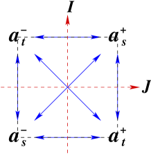
Figure 1: This figure summarizes the ${\hat{a}}^{\pm}_{s}$ and ${\hat{a}}^{\pm}_{t}$. Each of which is a member of simultaneous spin and isospin $j=1/2$ multiplet. ${\hat{J}}_{-}$ will bring ${\hat{a}}^{+}_{s}$ down to ${\hat{a}}^{-}_{t}$ and ${\hat{I}}_{+}$ moves ${\hat{a}}^{-}_{s}$ up to ${\hat{a}}^{-}_{t}$ etc.

Can the situation be salvaged somehow? How about simply dropping all the unphysical states from Eq. (LABEL:eq:nots) or imagine that we have a projection operator $\hat{\cal P}$ at our disposal, which when applied to $|\psi,a^{\mathbb{C}}\rangle$, projects out only the physical states

$$|\Psi,a^{\mathbb{C}}\rangle = \hat{\cal P}|\psi,a^{\mathbb{C}}\rangle$$

$$= \sum_{j,m,n\in{\mathbb{Z}}+1/2}e^{-\frac{1}{2\lambda\omega}j(j+1)}|j,m,n\rangle\langle j,m,n|a^{\mathbb{C}}\rangle\;.$$

In Ref. me1 an argument in terms of the wavefunction representation as to why this would not work was presented. Here we shall instead rely on the algebra of $S^{3}$. The form of Eq. (27) requires us to know how ${\hat{a}}_{b}$ acts on the states $|j,m,n\rangle$. In the Appendix B some algebra of ${\hat{J}}_{i}$ and ${\hat{I}}_{i}$ with ${\hat{a}}_{b}$ have been worked out. It is convenient to use the combination

$$\hat{a}^{\pm}_{s}={\hat{a}}_{1}\pm i{\hat{a}}_{2}\;,\;\;\;\hat{a}^{\pm}_{t}={\hat{a}}_{0}\pm i{\hat{a}}_{3}\;.$$ (53)

The algebra shows that they raise or lower the third component of spin and isospin of $|j,m,n\rangle$ by $1/2$. For example

$${\hat{J}}_{3}\hat{a}^{\pm}_{s}|j,m,n\rangle = (m\pm\frac{1}{2})\;\hat{a}^{\pm}_{s}|j,m,n\rangle$$ (54)

$${\hat{I}}_{3}\hat{a}^{\pm}_{t}|j,m,n\rangle = (n\mp\frac{1}{2})\;\hat{a}^{\pm}_{t}|j,m,n\rangle$$ (55)

but the ${\hat{a}}|j,m,n\rangle$’s are not eigenstates of ${\hat{J}}^{2}$ and ${\hat{I}}^{2}$ in general (see Eq. (107)). The algebra can succinctly summarized by Fig. 1. This shows that each of the ${\hat{a}}^{\pm}_{s}$ and ${\hat{a}}^{\pm}_{t}$ belongs to a simultaneous spin-$1/2$ and isospin-$1/2$ doublets.

Their actions on the state vectors in general are

$$\hat{a}^{\pm}_{s}|j,m,n\rangle = C_{s}^{\pm}(j,m,n,+)|j+{\scriptstyle\frac{1}{2}},m\pm{\scriptstyle\frac{1}{2}},n\pm{\scriptstyle\frac{1}{2}}\rangle$$

$$+C_{s}^{\pm}(j,m,n,-)|j-{\scriptstyle\frac{1}{2}},m\pm{\scriptstyle\frac{1}{2}},n\pm{\scriptstyle\frac{1}{2}}\rangle$$

$$\hat{a}^{\pm}_{t}|j,m,n\rangle = C_{t}^{\pm}(j,m,n,+)|j+{\scriptstyle\frac{1}{2}},m\pm{\scriptstyle\frac{1}{2}},n\mp{\scriptstyle\frac{1}{2}}\rangle$$

$$+C_{t}^{\pm}(j,m,n,-)|j-{\scriptstyle\frac{1}{2}},m\pm{\scriptstyle\frac{1}{2}},n\mp{\scriptstyle\frac{1}{2}}\rangle$$

where $C_{s}^{\pm}$ and $C_{t}^{\pm}$ are numerical coefficients and functions of ($j,m,n$). These equations can be formally deduced from the algebra of the $SU(2)$ collectively quantized operators. These are given in Appendix B. However the simplest way to see this is to use the observation that each $a_{s}^{\pm}$ and $a_{t}^{\pm}$ is a member of a doublet. Therefore they have $j=1/2$ and $m=n=\pm 1/2$. The eigenstate on which the operators act also has its own value of $j,m,n$. The operators and the state thus form a direct product which can be decomposed as a direct sum of state with new total spin and isospin eigenvalues $j+1/2$ and $j-1/2$

$$j\otimes 1/2=(j+1/2)\oplus(j-1/2)\;.$$ (58)

This results naturally in Eqs. (LABEL:eq:as|st) and (LABEL:eq:at|st). In Appendix C more details are given. Also given there are the necessary steps to solve for the coefficients $C^{\pm}_{s}$ and $C^{\pm}_{t}$.

Acting on Eq. (LABEL:eq:cbs?) with ${\hat{a}}_{b}$ is to turn every half-integral spin state in the expansion into integral spin state. Therefore Eq. (LABEL:eq:cbs?) is not an eigenstate of Eq. (49). Keeping only physical states in the expansion does not solve the problem.

VI Coherent States with $SO(3)$ Operators on the $S^{3}$ Manifold

We have seen that the problem of constructing coherent state using the $SU(2)$ collective quantization and that the $SO(3)$ quantization giving only unphysical states. Thus neither approach permits the identification of the coherent states as the quantum analog of the classical skyrmions. Nevertheless there is a way out. As discussed in Ref. me1 the reason that the $SU(2)$ theory fails was because of the $SU(2)$ operators mapped fermions to bosons and vice versa. Therefore the $SU(2)$ annihilation operators require the full set of bosonic and fermionic states. However if we act on the Hilbert space of the $SU(2)$ quantized theory exclusively with combinations of ${\hat{a}}_{i}{\hat{a}}_{j}$, this would map fermions to fermions and bosons to bosons. The fermion part and the boson part of the Hilbert space therefore decouple and the latter can be eliminated. This is achieved by “mixing” the $SU(2)$ and $SO(3)$ theory. One discards the $SO(3)$ Hilbert space but keeps the operators and at the same time keeps the Hilbert space (only the fermion half of it) of the $SU(2)$ theory but discards the operators.

According to the description in Sec. IV.1 after introducing an energy scale $\omega$, from Eq. (17) the complexifier for the $SO(3)$ system is

$$C=\frac{1}{\lambda\omega}\Pi_{ij}\Pi_{ij}=\frac{1}{2\lambda\omega}J^{2}\;.$$ (59)

The annihilation operators based on the $SO(3)$ coordinate operators ${\hat{R}}_{ij}$ are therefore

$$\hat{A}_{ij}=e^{-\frac{1}{2\lambda\omega}{\hat{J}}^{2}}{\hat{R}}_{ij}e^{\frac{1}{2\lambda\omega}{\hat{J}}^{2}}\;.$$ (60)

Just like in the $SU(2)$ quantization, the $\hat{A}_{ij}$ can be expressed in another form by expanding the exponential and then regrouping the terms. This will bring them to a more traditional form. Using the $SO(3)$ algebra in Appendix F, this other form is derived in Appendix G.

The coherent states are constructed from a complex labeled position state $|a^{\mathbb{C}}\rangle$ on $S^{3}_{\mathbb{C}}$ as before. This should be an eigenstate of the position operators ${\hat{R}}_{ij}$. How do the ${\hat{R}}_{ij}$ act on $|a^{\mathbb{C}}\rangle$? Recall that the $R_{ij}$ although are elements in the $3\times 3$ rotation matrix $R$, they are not completely dissociated from the $a_{b}$ of the $SU(2)$ element $A$. In fact as shown in me2 , $R_{ij}=R_{ij}(A)=R_{ij}(a)$ so

$${\hat{R}}_{ij}|a^{\mathbb{C}}\rangle=R_{ij}(a^{\mathbb{C}})|a^{\mathbb{C}}\rangle\;.$$ (61)

The position states $|a^{\mathbb{C}}\rangle$ are indeed eigenstates of ${\hat{R}}_{ij}$. Therefore the method together with the above discussion give us

$$|\Psi,a^{\mathbb{C}}\rangle=\hat{\cal P}e^{-\frac{1}{2\lambda\omega}{\hat{J}}^{2}}|a^{\mathbb{C}}\rangle$$ (62)

as the coherent states. So with Eq. (60) as the annihilation operators we have

$$\hat{A}_{ij}|\Psi,a^{\mathbb{C}}\rangle=R_{ij}(a^{\mathbb{C}})|\Psi,a^{\mathbb{C}}\rangle\;.$$ (63)

To obtain these states in terms of the eigenstates $|j,m,n\rangle$, one insert a “complete” set of states in the fermionic space to recover Eq. (LABEL:eq:cbs?). So finally the coherent states consist only of baryon and excited baryon states that we have been looking for and identifiable with the classical skyrmions.

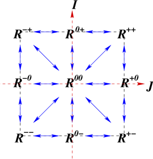
Figure 2: This figure summarizes at least two important facts. The first being the action of ${\hat{J}}_{i}$ and ${\hat{I}}_{i}$ on the nine combinations of ${\hat{R}}_{ij}$. They form three overlapping spin and three isospin triplets. For example ${\hat{J}}^{+}$ brings ${\hat{R}}^{00}$ horizontally to ${\hat{R}}^{+0}$ and ${\hat{I}}^{-}$ brings ${\hat{R}}^{-+}$ vertically down to ${\hat{R}}^{-0}$ etc (see algebra in Appendix Eq. (150). Each member is simultaneously in one spin and one isospin multiplet. The second is how these combinations act on the states (see text). For example ${\hat{R}}^{++}$ raises both the third component of spin $m$ and isospin $n$ by one, ${\hat{R}}^{-0}$ lowers $m$ by one but leaves $n$ alone.

VII A mixed quantum system of $SO(3)$ operators and $SU(2)$ Hilbert Space

To permit ourselves to verify explicitly the eigenvalue equations and to familiarize with this mixed operator-state system, we will derive the action of the $SO(3)$ operators on the $SU(2)$ eigenstates. This can be rigorously deduced from the algebra of the $SO(3)$ operators. They are given in the Appendix F. From the algebra, again one can find useful combinations of the components $R_{ij}$. These have been given in me2 and repeated in operator form in Appendix F. Each $R^{pq}$ with $p,q=\pm,0$ is a sum of components $R_{ij}$ and belongs simultaneously to one spin and one isospin triplet (see Fig. 2). Using similar argument as before, the action of $R^{pq}$ on an eigenstate $|j,m,n\rangle$ results in a direct product between the operator and the state which can be decomposed as

$$j\otimes 1=(j+1)\oplus j\oplus(j-1)\;.$$ (64)

Therefore we must have

$${\hat{R}}^{pq}|j,m,n\rangle = \;\;C^{pq}(j,m,n,+)|j+1,m+p1,n+q1\rangle$$

$$+C^{pq}(j,m,n,0)|j,m+p1,n+q1\rangle$$

$$+C^{pq}(j,m,n,-)|j-1,m+p1,n+q1\rangle\;.$$

The $p1,q1$ objects need some explanations. The $p,q$ are the superscript of $R^{pq}$ and are signs equal to $+$, $-$ or 0. $p1$ means the sign $p$ multiplying with $1$. If $p$ is equal to $+,-$ or $0$, then $p1=+1$, $-1$ or $0$ respectively. The same applies to $q1$. The coefficients $C^{pq}$ are solved and listed in Appendix H and I respectively. The actions of $\Pi^{pq}$ on $|j,m,n\rangle$ can be similarly expressed but with different coefficients.

Expectation values are an integral part of any quantum system and it is most convenient of work in terms of wavefunctions. The position wavefunction of the coherent state labeled by $a^{\mathbb{C}}$ on $S^{3}$ at the point $b=(b_{0},b_{1},b_{2},b_{3})$ on $S^{3}$ would be (up to normalization)

$$\Psi_{a^{\mathbb{C}}}(b)=\langle b|\Psi,a^{\mathbb{C}}\rangle\;.$$ (66)

We use ${\hat{R}}_{ij}$ for position operators so the expectation value of “position” would be

$$\langle\Psi,a^{\mathbb{C}}|{\hat{R}}_{ij}|\Psi,a^{\mathbb{C}}\rangle=\int d^{4}b\;\delta(1-b_{c}^{2})\;R_{ij}(b)|\Psi_{a^{\mathbb{C}}}(b)|^{2}\;.$$ (67)

This might cause some confusion because the wavefunctions are on $S^{3}$ while the expectation values are of the $SO(3)$ operators. In general expectation values of an operator $\hat{O}$ from the $SO(3)$ quantized theory in a coherent state is

$$\langle\Psi,a^{\mathbb{C}}|\hat{O}|\Psi,a^{\mathbb{C}}\rangle=\int d^{4}b\;\delta(1-b_{c}^{2})\;\Psi_{a^{\mathbb{C}}}(b)^{*}\,\hat{O}\,\Psi_{a^{\mathbb{C}}}(b)\;.$$ (68)

VIII Classical Skyrmion as a Coherent Superposition of Baryon and Higher Resonance States

Given that the coherent states are of the form

$$|\Psi,a^{\mathbb{C}}\rangle=\hat{\cal P}e^{-\frac{1}{2\lambda\omega}{\hat{J}}^{2}}|a^{\mathbb{C}}\rangle\;,$$ (69)

inserting a complete set of fermion states and they can be written in terms only of baryon states as

$$|\Psi,a^{\mathbb{C}}\rangle = \sum_{j,m,n\in{\mathbb{Z}}+1/2}e^{-\frac{1}{2\lambda\omega}j(j+1)}|j,m,n\rangle\langle j,m,n|a^{\mathbb{C}}\rangle$$

$$= \sum_{j,m,n\in{\mathbb{Z}}+1/2}e^{-\frac{1}{2\lambda\omega}j(j+1)}\psi^{*}_{jmn}(a^{\mathbb{C}})|j,m,n\rangle\;.$$

$\psi_{jmn}(a)$ again are the baryon wavefunctions on $S^{3}$ and $\psi^{*}_{jmn}(a^{\mathbb{C}})$ are the complex conjugates of these wavefunctions evaluated at the complex point $a^{\mathbb{C}}$.

Let us see some explicit examples of what the states look like. Using the wavefunctions for $p,n$ ($j=1/2$) and $\Delta$ ($j=3/2$), the baryonic coherent state with label $a^{\mathbb{C}}=\beta=(0,1,0,0)$ is

$$|\Psi,\beta\rangle = \frac{e^{-\frac{3}{8\lambda\omega}}}{\pi}\Big{(}|p,{\scriptstyle\frac{1}{2}}\rangle-|n,{\scriptstyle-\frac{1}{2}}\rangle\Big{)}+\frac{\sqrt{2}e^{-\frac{15}{8\lambda\omega}}}{\pi}\Big{(}|\Delta^{++},{\scriptstyle\frac{3}{2}}\rangle-|\Delta^{+},{\scriptstyle\frac{1}{2}}\rangle+|\Delta^{0},{\scriptstyle-\frac{1}{2}}\rangle-|\Delta^{-},{\scriptstyle-\frac{3}{2}}\rangle\Big{)}+\dots\;.$$ (71)

The ellipses denote half-integral spin higher states. In this case the nucleons have the same probability and this is similarly true among the $\Delta$ in the superposition. The spin and isospin are correlated by $m=n$ in this special case.

With a different label $a^{\mathbb{C}}=\gamma=(\gamma_{0},0,0,\gamma_{3})$ where $\gamma_{0}$ and $\gamma_{3}$ are in general complex numbers satisfying $\gamma_{0}^{2}+\gamma_{3}^{2}=1$, the state is

$$|\Psi,\gamma\rangle = \frac{ie^{-\frac{3}{8\lambda\omega}}}{\pi}\Big{(}(\gamma_{0}+i\gamma_{3})|p,{\scriptstyle-\frac{1}{2}}\rangle-(\gamma_{0}-i\gamma_{3})|n,{\scriptstyle\frac{1}{2}}\rangle\Big{)}$$ (72)

$$- \frac{i\sqrt{2}e^{-\frac{15}{8\lambda\omega}}}{\pi}\Big{(}(\gamma_{0}+i\gamma_{3})^{3}|\Delta^{++},{\scriptstyle-\frac{3}{2}}\rangle-(\gamma_{0}+i\gamma_{3})|\Delta^{+},{\scriptstyle-\frac{1}{2}}\rangle+(\gamma_{0}-i\gamma_{3})|\Delta^{0},{\scriptstyle\frac{1}{2}}\rangle-(\gamma_{0}-i\gamma_{3})^{3}|\Delta^{-},{\scriptstyle\frac{3}{2}}\rangle\Big{)}$$

$$+ \dots\;.$$

Recalling that $\gamma_{i}$ are complex so this time both the nucleons and the deltas do not have the same probabilities. This is true in general. However the special choice of the label $\gamma$ ensures that this is a different correlation $m=-n$ in the superposition.

It should be clear that the expectation values of these states depend in general on the label. For example

$$\langle\Psi,\beta|{\hat{J}}_{i}|\Psi,\beta\rangle=\langle\Psi,\beta|{\hat{I}}_{i}|\Psi,\beta\rangle=0$$ (73)

but

$$\langle\Psi,\gamma|{\hat{J}}_{3}|\Psi,\gamma\rangle=\langle\Psi,\gamma|{\hat{I}}_{3}|\Psi,\gamma\rangle\neq 0\;.$$ (74)

In the chiral bag soliton type model ct ; gr ; bir ; fug ; ueh , the construction often involves the restriction of “grand spin” to

$$({\hat{J}}_{i}+{\hat{I}}_{i})|\psi\rangle=0$$ (75)

for minimizing the energy of the hedgehog state fug . From the last expression this can, if need be, be imposed by setting $\gamma_{1}=\gamma_{2}=\gamma_{3}=0$ and $\gamma_{0}=1$.

To determine the probability of baryons being produced from skyrmion in DCC formation, one can calculate the relative probability for a given baryonic coherent state from the general expression for the states above. The relative weights between nucleons and Deltas in a state with a given label $a^{\mathbb{C}}$ is therefore given by

$$\frac{{\cal P}_{\Delta}(a^{\mathbb{C}})}{{\cal P}_{N}(a^{\mathbb{C}})}=e^{-\frac{3}{\lambda\omega}}\frac{\sum_{m,n}\psi^{*}_{3/2,m,n}({a^{{\mathbb{C}}}}^{*})\psi_{3/2,m,n}(a^{\mathbb{C}})}{\sum_{m,n}\psi^{*}_{1/2,m,n}({a^{{\mathbb{C}}}}^{*})\psi_{1/2,m,n}(a^{\mathbb{C}})}\;.$$ (76)

The relative probabilities of other higher states can be worked out in a similar manner. In the first example with $a^{\mathbb{C}}=\beta$, the relative probability between deltas and nucleons is particularly simple

$$\frac{{\cal P}_{\Delta}(\beta)}{{\cal P}_{N}(\beta)}=4\;e^{-\frac{3}{\lambda\omega}}\;.$$ (77)

In the second case where $a^{\mathbb{C}}=\gamma$, let us take Im$\gamma_{0}=$Re$\gamma_{3}=0$, Re$\gamma_{0}=\mu$ and Im$\gamma_{3}=\nu=\sqrt{\mu^{2}-1}$ then

$$\frac{{\cal P}_{\Delta}(\gamma)}{{\cal P}_{N}(\gamma)}=e^{-\frac{3}{\lambda\omega}}\left(\frac{(\mu+\nu)^{6}+(\mu-\nu)^{6}+(\mu+\nu)^{2}+(\mu-\nu)^{2}}{(\mu+\nu)^{2}+(\mu-\nu)^{2}}\right)\;.$$ (78)

This shows that in general the expression can be quite complicated but mostly one would be interested in the numerical values and these can be worked out from the formula provided $\lambda$ and $\omega$ are fixed. The former can be estimated from the mass of the nucleon, of the delta and the pion decay constant. The latter is not known but a rough guess would be the energy scale of the chiral phase transition or the value of the temperature $T_{c}$.

IX Summary and Outlook

We have argued that the classical skyrmion solutions can be identified with their quantum analogs, namely coherent states of baryons. Due to the non-linear nature of the Skyrme model, the space of the states is the curved, compact space of $S^{3}$. Using the method of Ref. ha ; tt0 ; tt1 ; kr ; krp ; hm specially suitable for compact manifolds, these special superposition states of baryons have been successfully constructed. The states and wavefunctions are exactly those derived by Adkin et al anw without modification including the unphysical states of integral spin and isospin fr . Since a skyrmion must be made up only of baryons, such states must completely be removed from the superposition that ultimately will be equated to the skyrmion. In order to overcome this problem, we find that it is necessary to bring in the operators from the lesser known $SO(3)$ collective quantization. Only with these integral spin and isospin operators can the fermionic and the bosonic part of the Hilbert space be decoupled. The unphysical states can therefore be discarded. The distribution of the baryon states of given quantum numbers in the superposition come in the form of the moduli square of the baryon wavefunction of the corresponding states weighed by an exponential factor. This factor depends on the ratio of the energy of the individual state and an energy scale fundamental to the problem. This scale have not been determined but we expect it to be of the value of the chiral phase transition temperature. With this successful completion of the decomposition of the skyrmion into know baryon states, we should be ready to apply this to study skyrmion formation from DCC in heavy ion collisions. This will be done in the near future me3 .

Appendix A Nucleon and Delta Wavefunctions

For nucleons,

$$\langle a|p,{\scriptstyle+\frac{1}{2}}\rangle\!\! = \!\!+\frac{1}{\pi}(a_{1}+ia_{2})$$ (79)

$$\langle a|p,{\scriptstyle-\frac{1}{2}}\rangle\!\! = \!\!-\frac{i}{\pi}(a_{0}-ia_{3})$$ (80)

$$\langle a|n,{\scriptstyle+\frac{1}{2}}\rangle\!\! = \!\!+\frac{i}{\pi}(a_{0}+ia_{3})$$ (81)

$$\langle a|n,{\scriptstyle-\frac{1}{2}}\rangle\!\! = \!\!-\frac{1}{\pi}(a_{1}-ia_{2})$$ (82)

For Deltas,

$$\langle a|\Delta^{++},{\scriptstyle+\frac{3}{2}}\rangle\!\! = \!\!\frac{\sqrt{2}}{\pi}(a_{1}+ia_{2})^{3}$$ (83)

$$\langle a|\Delta^{+},{\scriptstyle+\frac{3}{2}}\rangle\!\! = \!\!i\frac{\sqrt{6}}{\pi}(a_{1}+ia_{2})^{2}(a_{0}+ia_{3})$$ (84)

$$\langle a|\Delta^{0},{\scriptstyle+\frac{3}{2}}\rangle\!\! = \!\!-\frac{\sqrt{6}}{\pi}(a_{1}+ia_{2})(a_{0}+ia_{3})^{2}$$ (85)

$$\langle a|\Delta^{-},{\scriptstyle+\frac{3}{2}}\rangle\!\! = \!\!-i\frac{\sqrt{2}}{\pi}(a_{0}+ia_{3})^{3}$$ (86)

$$\langle a|\Delta^{++},{\scriptstyle+\frac{1}{2}}\rangle\!\! = \!\!-i\frac{\sqrt{6}}{\pi}(a_{1}+ia_{2})^{2}(a_{0}-ia_{3})$$ (87)

$$\langle a|\Delta^{+},{\scriptstyle+\frac{1}{2}}\rangle\!\! = \!\!-\frac{\sqrt{2}}{\pi}(a_{1}+ia_{2})(1-3(a_{0}^{2}+a_{3}^{2}))$$

$$\langle a|\Delta^{0},{\scriptstyle+\frac{1}{2}}\rangle\!\! = \!\!i\frac{\sqrt{2}}{\pi}(a_{0}+ia_{3})(1-3(a_{1}^{2}+a_{2}^{2}))$$

$$\langle a|\Delta^{-},{\scriptstyle+\frac{1}{2}}\rangle\!\! = \!\!\frac{\sqrt{6}}{\pi}(a_{1}-ia_{2})(a_{0}+ia_{3})^{2}$$ (90)

$$\langle a|\Delta^{++},{\scriptstyle-\frac{1}{2}}\rangle\!\! = \!\!-\frac{\sqrt{6}}{\pi}(a_{1}+ia_{2})(a_{0}-ia_{3})^{2}$$ (91)

$$\langle a|\Delta^{+},{\scriptstyle-\frac{1}{2}}\rangle\!\! = \!\!-i\frac{\sqrt{2}}{\pi}(a_{0}-ia_{3})(1-3(a_{1}^{2}+a_{2}^{2}))$$

$$\langle a|\Delta^{0},{\scriptstyle-\frac{1}{2}}\rangle\!\! = \!\!\frac{\sqrt{2}}{\pi}(a_{1}-ia_{2})(1-3(a_{0}^{2}+a_{3}^{2}))$$ (93)

$$\langle a|\Delta^{-},{\scriptstyle-\frac{1}{2}}\rangle\!\! = \!\!i\frac{\sqrt{6}}{\pi}(a_{1}-ia_{2})^{2}(a_{0}+ia_{3})$$ (94)

$$\langle a|\Delta^{++},{\scriptstyle-\frac{3}{2}}\rangle\!\! = \!\!i\frac{\sqrt{2}}{\pi}(a_{0}-ia_{3})^{3}$$ (95)

$$\langle a|\Delta^{+},{\scriptstyle-\frac{3}{2}}\rangle\!\! = \!\!\frac{\sqrt{6}}{\pi}(a_{0}-ia_{3})^{2}(a_{1}-ia_{2})$$ (96)

$$\langle a|\Delta^{0},{\scriptstyle-\frac{3}{2}}\rangle\!\! = \!\!-i\frac{\sqrt{6}}{\pi}(a_{1}-ia_{2})^{2}(a_{0}-ia_{3})$$ (97)

$$\langle a|\Delta^{-},{\scriptstyle-\frac{3}{2}}\rangle\!\! = \!\!-\frac{\sqrt{2}}{\pi}(a_{1}-ia_{2})^{3}$$ (98)

Appendix B The Algebra on $S^{3}$

In the text the action of $J_{i}$ and $I_{i}$ on $a_{b}$ are required. From Eq. (9) the commutator between the rotation generators (angular momenta)

$${\hat{L}}_{bc}={\hat{a}}_{b}{\hat{\pi}}_{c}-{\hat{a}}_{c}{\hat{\pi}}_{b}$$ (99)

and ${\hat{a}}_{b}$ can be deduced

$$[\hat{L}_{bc},{\hat{a}}_{d}]=i(\delta_{bd}{\hat{a}}_{c}-\delta_{cd}{\hat{a}}_{b})\;.$$ (100)

It follows that the spin and isospin operators and ${\hat{a}}_{b}$ satisfy

$$[{\hat{J}}_{i},{\hat{a}}_{0}] =\;\;\;\frac{1}{2}i{\hat{a}}_{i}\;,\;\;[{\hat{I}}_{i},{\hat{a}}_{0}] =-\frac{1}{2}i{\hat{a}}_{i}$$ (101)

$${}[{\hat{J}}_{i},{\hat{a}}_{i}] =-\frac{1}{2}i{\hat{a}}_{0}\;,\;\;[{\hat{I}}_{i},{\hat{a}}_{i}] =\;\;\;\frac{1}{2}i{\hat{a}}_{0}$$ (102)

$${}[{\hat{J}}_{i},{\hat{a}}_{j}] =\frac{1}{2}i\epsilon_{ijk}{\hat{a}}_{k}\;,\;\;[{\hat{I}}_{i},{\hat{a}}_{j}] =\frac{1}{2}i\epsilon_{ijk}{\hat{a}}_{k}\;.$$ (103)

These can be written more compactly as

$$[\hat{J}_{i},{\hat{a}}_{b}] = \mbox{$\frac{1}{2}$}i(\delta_{b0}{\hat{a}}_{i}-\delta_{ib}{\hat{a}}_{0}+\delta_{bj}\epsilon_{ijk}{\hat{a}}_{k})$$ (104a)

$${}[\hat{I}_{i},{\hat{a}}_{b}] = \mbox{$\frac{1}{2}$}i(\delta_{ib}{\hat{a}}_{0}-\delta_{b0}{\hat{a}}_{i}+\delta_{bj}\epsilon_{ijk}{\hat{a}}_{k})\;.$$ (104b)

In this form, they are not particularly useful. Let us write instead

$${\hat{a}}^{\pm}_{s}={\hat{a}}_{1}\pm i{\hat{a}}_{2}\;,\;\;\;\;{\hat{a}}^{\pm}_{t}={\hat{a}}_{0}\pm i{\hat{a}}_{3}\;.$$ (105)

These commute with each other because the ${\hat{a}}_{b}$’s do. Their action with respect to spin and isospin are dictated and made clear by the following algebra

$$[{\hat{J}}_{\pm},\hat{a}^{\pm}_{s}] =\;\;0\;,\;\;\;\;\;\;\;[{\hat{I}}_{\pm},\hat{a}^{\pm}_{s}] =0$$ (106a)

$${}[{\hat{J}}_{\pm},\hat{a}^{\mp}_{s}] =-i\hat{a}^{\pm}_{t}\;,\;\;[{\hat{I}}_{\pm},\hat{a}^{\mp}_{s}] =i\hat{a}^{\mp}_{t}$$ (106b)

$${}[{\hat{J}}_{\pm},\hat{a}^{\pm}_{t}] =\;\;0\;,\;\;\;\;\;\;\;[{\hat{I}}_{\pm},\hat{a}^{\mp}_{t}] =0$$ (106c)

$${}[{\hat{J}}_{\pm},\hat{a}^{\mp}_{t}] =\;i\hat{a}^{\pm}_{s}\;,\;\;\;[{\hat{I}}_{\pm},\hat{a}^{\pm}_{t}] =-i\hat{a}^{\pm}_{s}$$ (106d)

$${}[{\hat{J}}_{3},\hat{a}^{\pm}_{s}] =\pm\frac{1}{2}\hat{a}^{\pm}_{s}\;,\;\;[{\hat{I}}_{3},\hat{a}^{\pm}_{s}] =\pm\frac{1}{2}\hat{a}^{\pm}_{s}$$ (106e)

$${}[{\hat{J}}_{3},\hat{a}^{\pm}_{t}] =\pm\frac{1}{2}\hat{a}^{\pm}_{t}\;,\;\;[{\hat{I}}_{3},\hat{a}^{\pm}_{t}] =\mp\frac{1}{2}\hat{a}^{\pm}_{t}\;.$$ (106f)

The last two lines show that $\hat{a}^{\pm}_{s}$ and $\hat{a}^{\pm}_{t}$ act like raising and lowering operators of one-half instead of the usual one with respect to the third component of spin and isospin. But states acted on by $\hat{a}^{\pm}_{s}$ and $\hat{a}^{\pm}_{t}$ are not eigenstates of ${\hat{J}}^{2}$ and ${\hat{I}}^{2}$ in general. The commutators are

$$[{\hat{J}}^{2},\hat{a}^{\pm}_{s}] = -i\hat{a}^{\mp}_{t}{\hat{J}}_{\pm}\pm\hat{a}^{\pm}_{s}({\hat{J}}_{3}\pm\frac{3}{4})$$ (107a)

$${}[{\hat{J}}^{2},\hat{a}^{\pm}_{t}] = \;\;\;i\hat{a}^{\mp}_{s}{\hat{J}}_{\pm}\pm\hat{a}^{\pm}_{t}({\hat{J}}_{3}\pm\frac{3}{4})$$ (107b)

$${}[{\hat{I}}^{2},\hat{a}^{\pm}_{s}] = \;\;\;i\hat{a}^{\pm}_{t}{\hat{I}}_{\pm}\pm\hat{a}^{\pm}_{s}({\hat{I}}_{3}\pm\frac{3}{4})$$ (107c)

$${}[{\hat{I}}^{2},\hat{a}^{\pm}_{t}] = -i\hat{a}^{\pm}_{s}{\hat{I}}_{\mp}\mp\hat{a}^{\pm}_{t}({\hat{I}}_{3}\mp\frac{3}{4})\;.$$ (107d)

Similarly one can work out the commutators with the conjugate momenta ${\hat{\pi}}_{b}$ to find out how they act on the states. Beginning with the four-dimensional rotation

$$[\hat{L}_{bc},{\hat{\pi}}_{d}]=i(\delta_{bd}{\hat{\pi}}_{c}-\delta_{cd}{\hat{\pi}}_{b})\;.$$ (108)

This is exactly Eq. (100) but with ${\hat{a}}_{b}$ replaced by ${\hat{\pi}}_{b}$. Therefore ${\hat{\pi}}_{b}$ must have the similar commutators with $J_{\pm}$, $J_{3}$, $I_{\pm}$ and $I_{3}$ as ${\hat{a}}_{b}$.

Appendix C Action of ${\hat{a}}_{b}$ on the Spin and Isospin States

In constructing coherent states on $S^{3}$, it is necessary to find out how the operators ${\hat{a}}_{b}$ act on the spin and isospin states $|j,m,n\rangle$. These are largely governed by the algebras given in Appendix B and the constraint Eq. (5). Naturally the operator form of the constraint

$${\hat{a}}_{b}{\hat{a}}_{b}={\hat{a}}^{+}_{s}{\hat{a}}^{-}_{s}+{\hat{a}}^{+}_{t}{\hat{a}}^{-}_{t}=1$$ (109)

is the Casimir operator. The action of ${\hat{a}}_{b}$ on the states must take that into account. It must also constrain the form that this action will take. From the algebra, one can see that they either increase or decrease the $m$ and $n$ by one-half. The effect on the total (iso)spin $j$ is however less clear. Although the action of $\hat{a}^{\pm}_{s}$ and $\hat{a}^{\pm}_{t}$ on the states give eigenstates of ${\hat{J}}_{3}$ and ${\hat{I}}_{3}$, these are not eigenstates of ${\hat{J}}^{2}$ or ${\hat{I}}^{2}$. Lengthy calculation using the algebra on $S^{3}$ does show that the ${\hat{a}}^{\pm}$ acting on a state with $j$ gives two states in general: one with $j+1/2$ and the other with $j-1/2$. Nevertheless this can also be deduced from a much simpler argument.

From the algebra in Appendix B, each ${\hat{a}}_{b}$ carries $j=1/2$ so decomposition of a direct product of a state with $j$ with $1/2$ gives the direct sum

$$j\otimes 1/2=(j+1/2)\oplus(j-1/2)\;.$$ (110)

Alternatively a state of total (iso)spin $j$ has a wavefunction which is a polynomial of degree $l=2j$ in $(a_{b}+ia_{c})$. Acting with ${\hat{a}}^{\pm}$ on the state wavefunction will give a polynomial of $l+1=2(j+1/2)$. This seems to indicate that a state with $j$ will become one with $j+1/2$ but this is not the complete story. Remember that there is the constraint Eq. (109), it is therefore always possible to combine ${\hat{a}}^{\pm}$ with one $a^{\mp}$ in the wavefunction to reduce some terms in the polynomial from degree $l$ to $l-1=2(j-1/2)$. As a result one must generally have both possibilities of $j+1/2$ and $j-1/2$. The action of ${\hat{a}}^{\pm}$ on the states can thus be written as

$$\hat{a}^{\pm}_{s}|j,m,n\rangle = C_{s}^{\pm}(j,m,n,+)|j+{\scriptstyle\frac{1}{2}},m\pm{\scriptstyle\frac{1}{2}},n\pm{\scriptstyle\frac{1}{2}}\rangle$$

$$+C_{s}^{\pm}(j,m,n,-)|j-{\scriptstyle\frac{1}{2}},m\pm{\scriptstyle\frac{1}{2}},n\pm{\scriptstyle\frac{1}{2}}\rangle$$

$$\hat{a}^{\pm}_{t}|j,m,n\rangle = C_{t}^{\pm}(j,m,n,+)|j+{\scriptstyle\frac{1}{2}},m\pm{\scriptstyle\frac{1}{2}},n\mp{\scriptstyle\frac{1}{2}}\rangle$$

$$+C_{t}^{\pm}(j,m,n,-)|j-{\scriptstyle\frac{1}{2}},m\pm{\scriptstyle\frac{1}{2}},n\mp{\scriptstyle\frac{1}{2}}\rangle\;.$$

where $C_{s}^{\pm}$ and $C_{t}^{\pm}$ are numerical functions of ($j,m,n$).

To solve for the coefficients, one uses the algebra in Eq. (106). For example Eqs. (106a) and (106c) acting on a state give relation connecting $C_{s}^{\pm}$ and $C_{t}^{\pm}$ to themselves within a (iso)spin multiplet and Eqs. (106b) and (106d) relate $C_{s}^{\pm}$ to $C_{t}^{\pm}$. Then from the complex conjugation of matrix elements

$$\langle j+q{\scriptstyle\frac{1}{2}},m\pm{\scriptstyle\frac{1}{2}},n\pm{\scriptstyle\frac{1}{2}}|\hat{a}^{\pm}_{s}|j,m,n\rangle^{\ast}$$

$$\;\;\;\;=\langle j,m,n|\hat{a}^{\mp}_{s}|j+q{\scriptstyle\frac{1}{2}},m\pm{\scriptstyle\frac{1}{2}},n\pm{\scriptstyle\frac{1}{2}}\rangle$$ (112a)

$$\langle j+q{\scriptstyle\frac{1}{2}},m\pm{\scriptstyle\frac{1}{2}},n\mp{\scriptstyle\frac{1}{2}}|\hat{a}^{\pm}_{t}|j,m,n\rangle^{\ast}$$

$$\;\;\;\;=\langle j,m,n|\hat{a}^{\mp}_{t}|j+q{\scriptstyle\frac{1}{2}},m\pm{\scriptstyle\frac{1}{2}},n\mp{\scriptstyle\frac{1}{2}}\rangle$$ (112b)

with $q=\pm$ and using Eq. (111), we arrive at the relations between the coefficient functions

$$C_{s}^{\pm}(j,m,n,q)^{\ast} = C_{s}^{\mp}(j+q{\scriptstyle\frac{1}{2}},m\pm{\scriptstyle\frac{1}{2}},n\pm{\scriptstyle\frac{1}{2}})$$ (113a)

$$C_{t}^{\pm}(j,m,n,q)^{\ast} = C_{t}^{\mp}(j+q{\scriptstyle\frac{1}{2}},m\pm{\scriptstyle\frac{1}{2}},n\mp{\scriptstyle\frac{1}{2}})\;.$$ (113b)

These relations together with Eq. (109) allow us to obtain up to an overall phase factor

$$C^{\pm}_{s}(j,m,n,+) = \pm\sqrt{\frac{(j\pm m+1)(j\pm n+1)}{2(j+1)(2j+1)}}$$ (114a)

$$C^{\pm}_{s}(j,m,n,-) = \mp\sqrt{\frac{(j\mp m)(j\mp n)}{2j(2j+1)}}$$ (114b)

$$C^{\pm}_{t}(j,m,n,+) = \mp i\sqrt{\frac{(j\pm m+1)(j\mp n+1)}{2(j+1)(2j+1)}}$$ (114c)

$$C^{\pm}_{t}(j,m,n,-) = \mp i\sqrt{\frac{(j\mp m)(j\pm n)}{2j(2j+1)}}\;.$$ (114d)

Appendix D Alternative Form of the $SU(2)$ Annihilation Operators

$SU(2)$ operators are not used in the final results for the coherent states. They are to be replaced by those from $SO(3)$. We will show, nevertheless, in this section and in the next that there is an alternate form of the annihilation operators and that which chosen form of the secondary constraint among the various available choices discussed in me2 is used does not affect the uniqueness of the annihilation operators. This implies in turn that there is no ambiguity as to the uniqueness of the coherent states that follow from the operators.

The alternate form has a much closer resemblance to those of the simple harmonic oscillator than the unfamiliar form of position operators sandwiched between two exponentials. The complexifier is

$$C=\frac{1}{2\lambda\omega}J^{2}=\frac{1}{2\lambda\omega}I^{2}\;.$$ (115)

The $\omega$ is a fundamental energy scale as discussed in the text. The spin and isospin operators are related to the rotation generators ${\hat{L}}_{bc}$ by

$${\hat{J}}_{i} = \frac{1}{2}({\hat{L}}_{0i}+\frac{1}{2}\varepsilon_{ijk}{\hat{L}}_{jk})$$ (116a)

$${\hat{I}}_{i} = \frac{1}{2}({\hat{L}}_{0i}-\frac{1}{2}\varepsilon_{ijk}{\hat{L}}_{jk})\;.$$ (116b)

The annihilation operators are therefore

$$\hat{A}_{b} = e^{-\frac{1}{2\lambda\omega}\hat{J}^{2}}\hat{a}_{b}\,e^{\frac{1}{2\lambda\omega}\hat{J}^{2}}$$ (117)

$$= \sum^{\infty}_{n=0}\frac{1}{n!}\Big{(}\frac{1}{2\lambda\omega}\Big{)}^{n}[{\hat{a}}_{b},{\hat{J}}^{2}]_{n}\;.$$ (118)

with $[\hat{A},\hat{B}]_{0}=\hat{A}$ and $[\hat{A},\hat{B}]_{n+1}=[[\hat{A},\hat{B}]_{n},\hat{C}]$ representing the repeated application of the commutator $n+1$ times as mentioned in the main text. Let us work out the first few commutators in the sum. We begin by using the basic commutator in Appendix B to deduce that the angular momentum operators have the commutators

$$[\hat{L}_{bc},{\hat{a}}_{d}]=i(\delta_{bd}{\hat{a}}_{c}-\delta_{cd}{\hat{a}}_{b})\;.$$ (119)

Then using (see the Appendix of me2 )

$${\hat{J}}^{2}=\frac{1}{8}{\hat{L}}_{bc}{\hat{L}}_{bc}\;,$$ (120)

one gets

$$[{\hat{a}}_{b},{\hat{J}}^{2}] = \frac{1}{4}i({\hat{L}}_{cb}{\hat{a}}_{c}+{\hat{a}}_{c}{\hat{L}}_{cb})$$ (121)

$$= \frac{1}{2}i\Big{(}{\hat{L}}_{cb}-\frac{1}{2}i(d-1)\delta_{cb}\Big{)}{\hat{a}}_{c}$$

$$= i({\cal M}{\hat{a}})_{b}\;.$$

The last line has been written as a matrix equation so that hm

$$[{\hat{a}}_{b},{\hat{J}}^{2}]_{n}=i^{n}({\cal M}^{n}{\hat{a}})_{b}\;.$$ (122)

This is true because

$$[{\hat{J}}^{2},{\hat{L}}_{bc}]=0\;.$$ (123)

The annihilation operators can therefore be expressed in terms of $\mathcal{M}$

$$\hat{A}_{b}=\Big{(}\mbox{\rm exp}\{\mbox{$\frac{i}{2\lambda\omega}$}{\cal M}\}{\hat{a}}\Big{)}_{b}\;.$$ (124)

Before proceeding further, we will introduce the parameter $\alpha$ which was used in me2 to distinguish between the three ways that the second class constraint derived from Eq. (5) can be implemented quantum mechanically. In brief one can choose among any of the three ${\hat{a}}_{b}{\hat{\pi}}_{b}=0$, ${\hat{\pi}}_{b}{\hat{a}}_{b}=0$ or ${\hat{a}}_{b}{\hat{\pi}}_{b}+{\hat{\pi}}_{b}{\hat{a}}_{b}=0$ forms. This results in the relation

$${\hat{\pi}}_{c}={\hat{a}}_{b}{\hat{L}}_{bc}+i\alpha{\hat{a}}_{c}={\hat{L}}_{bc}{\hat{a}}_{b}+i(\alpha-d+1){\hat{a}}_{c}$$ (125)

between ${\hat{\pi}}_{b}$ and ${\hat{L}}_{bc}$. The corresponding value of $\alpha$ is given by $\alpha=0$, $\alpha=(d-1)$ and $\alpha=(d-1)/2$ respectively.

Using Eq. (125), one can work out

$$({\cal M}{\hat{a}})_{b}=\frac{1}{2}\Big{\{}{\hat{\pi}}_{b}-i\Big{(}\alpha-\frac{1}{2}(d-1)\Big{)}{\hat{a}}_{b}\Big{\}}\;.$$ (126)

The appearance of ${\hat{\pi}}_{b}$ here indicates that there is also the need of $[{\hat{\pi}}_{b},{\hat{J}}^{2}]$. The commutator of ${\hat{\pi}}_{b}$ with ${\hat{L}}$ is similar to that with ${\hat{a}}_{b}$

$$[\hat{L}_{bc},{\hat{\pi}}_{d}]=i(\delta_{bd}{\hat{\pi}}_{c}-\delta_{cd}{\hat{\pi}}_{b})$$ (127)

because the ${\hat{L}}$ are generators of four-dimensional rotations. The commutators are

$$[{\hat{\pi}}_{b},{\hat{J}}^{2}] = \frac{1}{4}i({\hat{L}}_{cb}{\hat{\pi}}_{c}+{\hat{\pi}}_{c}{\hat{L}}_{cb})$$ (128)

$$= \frac{1}{2}i\Big{(}{\hat{L}}_{cb}-\frac{1}{2}i(d-1)\delta_{cb}\Big{)}{\hat{\pi}}_{c}$$

$$= i({\cal M}{\hat{\pi}})_{b}\;.$$

The last line can be worked out explicitly using Eq. (125)

$$({\cal M}{\hat{\pi}})_{b} = \frac{1}{2}({\hat{\pi}}_{b}{\hat{a}}_{c}{\hat{\pi}}_{c}-{\hat{\pi}}_{c}{\hat{\pi}}_{c}{\hat{a}}_{b}+i{\hat{\pi}}_{c}{\hat{a}}_{c}{\hat{a}}_{b})-\frac{1}{4}i(d+1){\hat{\pi}}_{b}$$ (129)

$$= -\frac{1}{2}({\hat{\pi}}_{c}{\hat{\pi}}_{c}+\alpha-d+1){\hat{a}}_{b}$$

$$+\frac{1}{2}i\Big{(}\alpha-\frac{1}{2}(d+1)\Big{)}{\hat{\pi}}_{b}\;.$$

It is favorable to replace ${\hat{\pi}}_{c}{\hat{\pi}}_{c}$ by ${\hat{J}}^{2}$ which can be achieved with Eq. (125). Contracting this equation by ${\hat{\pi}}_{c}$ from the left gives

$${\hat{\pi}}_{c}{\hat{\pi}}_{c}=4{\hat{J}}^{2}-\alpha(\alpha-d+1)\hat{1}\;.$$ (130)

Then

$$({\cal M}{\hat{\pi}})_{b} = -\frac{1}{2}\Big{(}4{\hat{J}}^{2}+(1-\alpha)(\alpha-d+1)\Big{)}{\hat{a}}_{b}$$ (131)

$$+\frac{1}{2}i\Big{(}\alpha-\frac{1}{2}(d+1)\Big{)}{\hat{\pi}}_{b}\;.$$

The explicit appearance of $\alpha$ indicates that the annihilation operators depend on which of the three choices are chosen as the quantum version of the secondary constraint. This is the potential non-uniqueness of $\hat{A}_{b}$ that we allured to at the beginning. This ambiguity will be addressed in the next subsection.

Following hm for the purpose of working out $\hat{A}$, we let

$${\hat{a}}=\begin{pmatrix}1\\ 0\end{pmatrix}\;,\;\;\;\;{\hat{\pi}}=\begin{pmatrix}0\\ 1\end{pmatrix}\;,$$

then the corresponding ${\cal M}$ is

$${\cal M}=\frac{1}{2}\Big{(}\begin{smallmatrix}-i(\alpha-\frac{1}{2}(d-1))&-(4{\hat{J}}^{2}+(1-\alpha)(\alpha-d+1))\\ 1&i(\alpha-\frac{1}{2}(d+1))\\ \end{smallmatrix}\Big{)}\;.$$ (132)

It is advantageous to introduce a shift ${\cal M}=\tilde{\cal M}-i{\mathbbm{1}}/4$.

$$\hat{A}_{b}=\mbox{\rm exp}\{\mbox{$\frac{1}{8\lambda\omega}$}\}\;(\mbox{\rm exp}\{\mbox{$\frac{i}{2\lambda\omega}$}\tilde{\cal M}\}{\hat{a}})_{b}$$ (133)

where

$$\tilde{\cal M}=\frac{1}{2}\Big{(}\begin{smallmatrix}-i(\alpha-\frac{1}{2}d)&-(4{\hat{J}}^{2}+(1-\alpha)(\alpha-d+1))\\ 1&i(\alpha-\frac{1}{2}d)\\ \end{smallmatrix}\Big{)}\;.$$ (134)

This form has the convenient property that on squaring, it yields a diagonal matrix

$$\tilde{\cal M}^{2}=-\Big{(}{\hat{J}}^{2}+\frac{1}{4}(\frac{d}{2}-1)^{2}\hat{1}\Big{)}{\mathbbm{1}}=-{\cal J}^{2}{\mathbbm{1}}\;.$$ (135)

Therefore this together with Eq. (126) will allow us to work out $\hat{A}_{b}$.

The series expansion of $\hat{A}_{b}$ can be most easily calculated by exploiting the diagonal form of Eq. (135). Clearly the even power terms are all diagonal in the column vectors representation of ${\hat{a}}$ and ${\hat{\pi}}$. The sum of even $n$ power terms will therefore be a series in ${\cal J}/2\lambda\omega$ multiplying the $n=0$ term which is just ${\hat{a}}_{b}$

$$\Big{(}1-\frac{\tilde{\cal M}^{2}}{2!(2\lambda\omega)^{2}}+\frac{\tilde{\cal M}^{4}}{4!(2\lambda\omega)^{4}}+\dots\Big{)}_{bc}{\hat{a}}_{c}$$ (136)

$$= \Big{(}1+\frac{{\cal J}^{2}}{2!(2\lambda\omega)^{2}}+\frac{{\cal J}^{4}}{4!(2\lambda\omega)^{4}}+\dots\Big{)}{\hat{a}}_{b}$$

$$= \cosh\Big{(}\frac{\cal J}{2\lambda\omega}\Big{)}{\hat{a}}_{b}\;.$$

This even power series is the hyperbolic cosine. The sum of odd power terms can be re-expressed as an even power series in $\cal M$ by taking one power of $\cal M$ to act on ${\hat{a}}_{b}$ separately

$$i\Big{(}\frac{\tilde{\cal M}}{2\lambda\omega}-\frac{\tilde{\cal M}^{3}}{3!(2\lambda\omega)^{3}}+\frac{\tilde{\cal M}^{5}}{5!(2\lambda\omega)^{5}}+\dots\Big{)}_{bc}{\hat{a}}_{c}$$ (137)

$$i\Big{(}\frac{1}{2\lambda\omega}-\frac{\tilde{\cal M}^{2}}{3!(2\lambda\omega)^{3}}+\frac{\tilde{\cal M}^{4}}{5!(2\lambda\omega)^{5}}+\dots\Big{)}_{bc}(\tilde{\cal M}{\hat{a}})_{c}$$

$$= i\Big{(}\frac{1}{2\lambda\omega}+\frac{{\cal J}^{2}}{3!(2\lambda\omega)^{3}}+\frac{{\cal J}^{4}}{5!(2\lambda\omega)^{5}}+\dots\Big{)}(\tilde{\cal M}{\hat{a}})_{b}$$

$$= i\frac{1}{\cal J}\sinh\Big{(}\frac{\cal J}{2\lambda\omega}\Big{)}(\tilde{\cal M}{\hat{a}})_{b}\;.$$

Since

$$(\tilde{\cal M}{\hat{a}})_{b}=\mbox{$\frac{1}{2}$}\pi_{b}-i(\alpha-\mbox{$\frac{1}{2}$}d)\alpha_{b}\;,$$ (138)

therefore finally this is

$$\hat{A}_{b} = e^{\text{$\frac{1}{8\lambda\omega}$}}\cosh\Big{(}\frac{{\cal J}}{2\lambda\omega}\Big{)}{\hat{a}}_{b}$$ (139)

$$+e^{\text{$\frac{1}{8\lambda\omega}$}}\frac{1}{2{\cal J}}\big{(}\alpha-\frac{1}{2}d\big{)}\sinh\Big{(}\frac{{\cal J}}{2\lambda\omega}\Big{)}{\hat{a}}_{b}$$

$$+ie^{\text{$\frac{1}{8\lambda\omega}$}}\frac{1}{2{\cal J}}\sinh\Big{(}\frac{{\cal J}}{2\lambda\omega}\Big{)}{\hat{\pi}}_{b}\;.$$

This is the closest form that the annihilation operators can be reduced to the familiar form of the SHO. As mentioned in Ref. me1 , the ${\hat{J}}$ dependent coefficients are peculiar to compact spaces.

Appendix E Are $\hat{A}_{b}$ dependent on the Choice of the Secondary Constraint?

The explicit $\alpha$ dependence means that this form of $\hat{A}_{b}$ is dependent on the exact choice of the secondary constraint. Apparently this would lead to a problem because it implies that the coherent states are also dependent on the choice of $\alpha$. In fact this is not the case in spite of the apparent evidence to the contrary. It is ${\hat{\pi}}_{b}$ which is dependent on $\alpha$ and not $\hat{A}_{b}$. This can easily be seen if one substitutes for ${\hat{\pi}}_{b}$ in Eq. (139).

1. The First Choice: $\alpha=0$

   With this choice, the conjugate momenta are related to the angular momenta via

   $${\hat{\pi}}_{c}={\hat{a}}_{b}{\hat{L}}_{bc}\;.$$ (140)

   This obviously satisfies the constraint ${\hat{a}}_{b}{\hat{\pi}}_{b}=0$. Then the annihilation operators are

   $$\hat{A}_{b} = e^{\text{$\frac{1}{8\lambda\omega}$}}\cosh\Big{(}\frac{{\cal J}}{2\lambda\omega}\Big{)}{\hat{a}}_{b}$$ (141)

   $$-e^{\text{$\frac{1}{8\lambda\omega}$}}\frac{d}{4{\cal J}}\sinh\Big{(}\frac{{\cal J}}{2\lambda\omega}\Big{)}{\hat{a}}_{b}$$

   $$+ie^{\text{$\frac{1}{8\lambda\omega}$}}\frac{1}{2{\cal J}}\sinh\Big{(}\frac{{\cal J}}{2\lambda\omega}\Big{)}{\hat{\pi}}_{b}$$

2. The Second Choice: $\alpha=d-1$

   The conjugate momenta are now given by

   $${\hat{\pi}}_{c}={\hat{L}}_{bc}{\hat{a}}_{b}={\hat{a}}_{b}{\hat{L}}_{bc}+i(d-1){\hat{a}}_{c}\;.$$ (142)

   Obviously ${\hat{\pi}}_{b}{\hat{a}}_{b}=0$ is satisfied. The form that $\hat{A}_{b}$ take is

   $$\hat{A}_{b} = e^{\text{$\frac{1}{8\lambda\omega}$}}\cosh\Big{(}\frac{{\cal J}}{2\lambda\omega}\Big{)}{\hat{a}}_{b}$$ (143)

   $$+e^{\text{$\frac{1}{8\lambda\omega}$}}\frac{1}{2{\cal J}}\big{(}\frac{1}{2}d-1\big{)}\sinh\Big{(}\frac{{\cal J}}{2\lambda\omega}\Big{)}{\hat{a}}_{b}$$

   $$+ie^{\text{$\frac{1}{8\lambda\omega}$}}\frac{1}{2{\cal J}}\sinh\Big{(}\frac{{\cal J}}{2\lambda\omega}\Big{)}{\hat{\pi}}_{b}$$

3. The Third Choice: $\alpha=(d-1)/2$

   This choice gives a symmetric expression for the conjugate momenta

   $${\hat{\pi}}_{c}=\frac{1}{2}({\hat{a}}_{b}{\hat{L}}_{bc}+{\hat{L}}_{bc}{\hat{a}}_{b})={\hat{a}}_{b}{\hat{L}}_{bc}+\frac{1}{2}i(d-1){\hat{a}}_{c}\;.$$ (144)

   The annihilation operators are

   $$\hat{A}_{b} = e^{\text{$\frac{1}{8\lambda\omega}$}}\cosh\Big{(}\frac{{\cal J}}{2\lambda\omega}\Big{)}{\hat{a}}_{b}$$ (145)

   $$-e^{\text{$\frac{1}{8\lambda\omega}$}}\frac{1}{4{\cal J}}\sinh\Big{(}\frac{{\cal J}}{2\lambda\omega}\Big{)}{\hat{a}}_{b}$$

   $$+ie^{\text{$\frac{1}{8\lambda\omega}$}}\frac{1}{2{\cal J}}\sinh\Big{(}\frac{{\cal J}}{2\lambda\omega}\Big{)}{\hat{\pi}}_{b}$$

Now rewrite $\pi_{b}$ in each case in terms of ${\hat{L}}_{bc}$ and ${\hat{a}}_{b}$ the $\hat{A}_{b}$ are identically given by

$$\hat{A}_{b} = e^{\text{$\frac{1}{8\lambda\omega}$}}\cosh\Big{(}\frac{{\cal J}}{2\lambda\omega}\Big{)}{\hat{a}}_{b}$$ (146)

$$-e^{\text{$\frac{1}{8\lambda\omega}$}}\frac{d}{4{\cal J}}\sinh\Big{(}\frac{{\cal J}}{2\lambda\omega}\Big{)}{\hat{a}}_{b}$$

$$+ie^{\text{$\frac{1}{8\lambda\omega}$}}\frac{1}{2{\cal J}}\sinh\Big{(}\frac{{\cal J}}{2\lambda\omega}\Big{)}{\hat{a}}_{b}{\hat{L}}_{bc}$$

in all cases so the $\alpha$ dependence cancels out. On $S^{3}$ the angular momenta ${\hat{L}}_{bc}$ are more fundamental than ${\hat{\pi}}_{b}$. The formers are independent on the choice $\alpha$ but not the latter me2 . It follows that the annihilation operators are independent of the choice of how to implement the second class constraint. It follows that the coherent states are independent of $\alpha$.

Appendix F The Algebra on $SO(3)$

The basic commutators of the spin and isospin operators with the components of the $SO(3)$ collective coordinates ${\hat{R}}_{ij}$ are

$$[{\hat{J}}_{i},{\hat{R}}_{jk}] = \;\;\,i\epsilon_{ijm}{\hat{R}}_{mk}$$ (147a)

$${}[{\hat{I}}_{i},{\hat{R}}_{jk}] = -i{\hat{R}}_{jm}\epsilon_{imk}$$ (147b)

After experimenting with the commutators of ${\hat{J}}^{\pm}$, ${\hat{J}}_{3}$, ${\hat{I}}^{\pm}$ and ${\hat{I}}_{3}$ with ${\hat{R}}_{ij}$, we find it useful to form the following

$${\hat{R}}^{++} = {\hat{R}}_{11}-{\hat{R}}_{22}+i({\hat{R}}_{12}+{\hat{R}}_{21})$$ (148a)

$${\hat{R}}^{+-} = {\hat{R}}_{11}+{\hat{R}}_{22}-i({\hat{R}}_{12}-{\hat{R}}_{21})$$ (148b)

$${\hat{R}}^{-+} = {\hat{R}}_{11}+{\hat{R}}_{22}+i({\hat{R}}_{12}-{\hat{R}}_{21})$$ (148c)

$${\hat{R}}^{--} = {\hat{R}}_{11}-{\hat{R}}_{22}-i({\hat{R}}_{12}+{\hat{R}}_{21})$$ (148d)

$${\hat{R}}^{\pm 0} = {\hat{R}}_{13}\pm i{\hat{R}}_{23}$$ (148e)

$${\hat{R}}^{0\pm} = {\hat{R}}_{31}\pm i{\hat{R}}_{32}$$ (148f)

$${\hat{R}}^{00}\; = {\hat{R}}_{33}\;.$$ (148g)

The superscripts are designed with the following algebras in mind

$$[{\hat{J}}_{3},{\hat{R}}^{+\pm}] =\;\;\,{\hat{R}}^{+\pm}\;, [{\hat{I}}_{3},{\hat{R}}^{\pm+}] =\;\;\,{\hat{R}}^{\pm+}\;,$$ (149a)

$${}[{\hat{J}}_{3},{\hat{R}}^{-\pm}] =-{\hat{R}}^{-\pm}\;, [{\hat{I}}_{3},{\hat{R}}^{\pm-}] =-{\hat{R}}^{\pm-}\;,$$ (149b)

$${}[{\hat{J}}_{3},{\hat{R}}^{\pm 0}] =\pm{\hat{R}}^{\pm 0}\;, [{\hat{I}}_{3},{\hat{R}}^{0\pm}] =\pm{\hat{R}}^{0\pm}\;,$$ (149c)

$${}[{\hat{J}}_{3},{\hat{R}}^{0\pm}] =0\;, [{\hat{I}}_{3},{\hat{R}}^{\pm 0}] =0\;,$$ (149d)

$${}[{\hat{J}}_{3},{\hat{R}}^{00}] =0\;, [{\hat{I}}_{3},{\hat{R}}^{00}] =0\;.$$ (149e)

It is clear that ${\hat{R}}^{++}$, ${\hat{R}}^{+-}$ and ${\hat{R}}^{+0}$ raise the third component of spin by one unit, ${\hat{R}}^{--}$, ${\hat{R}}^{-+}$ and ${\hat{R}}^{-0}$ lower that by one unit. Also ${\hat{R}}^{++}$, ${\hat{R}}^{-+}$ and ${\hat{R}}^{0+}$ raise the third component of isospin by one and ${\hat{R}}^{--}$, ${\hat{R}}^{+-}$ and ${\hat{R}}^{0-}$ lower that by one. ${\hat{R}}^{\pm 0}$ and ${\hat{R}}^{0\pm}$ leave the third component of isospin and spin respectively alone. Finally ${\hat{R}}^{00}$ leaves the third component of both spin and isospin unchanged. The first and second superscripts show how the value of $m$ and $n$ respectively will be modified. Unlike the $SU(2)$ operators where ${\hat{a}}_{b}$ change $m$ and $n$ in steps of one-half, the ${\hat{R}}_{ij}$ change them by one unit at a time. The half unit increment or decrement is the source of the problem in $SU(2)$ which effectively couples the boson states with the fermion states under ${\hat{a}}_{b}$. With the $\Delta m=\Delta n=\pm 1$, one should now be able to cleanly separate the fermionic Hilbert space from the bosonic part.

The remaining commutation relations in terms of ${\hat{I}}_{\pm}$ and ${\hat{J}}_{\pm}$ are

$$[{\hat{J}}_{+},{\hat{R}}^{+\pm}] =0\;, [{\hat{I}}_{+},{\hat{R}}^{\pm+}] =0$$ (150a)

$${}[{\hat{J}}_{-},{\hat{R}}^{-\pm}] =0\;, [{\hat{I}}_{-},{\hat{R}}^{\pm-}] =0$$ (150b)

$${}[{\hat{J}}_{+},{\hat{R}}^{-\pm}] =\;\;2{\hat{R}}^{0\pm}\;, [{\hat{I}}_{+},{\hat{R}}^{\pm-}] =\;\;2{\hat{R}}^{\pm 0}$$ (150c)

$${}[{\hat{J}}_{-},{\hat{R}}^{+\pm}] =-2{\hat{R}}^{0\pm}\;, [{\hat{I}}_{-},{\hat{R}}^{\pm+}] =-2{\hat{R}}^{\pm 0}$$ (150d)

$${}[{\hat{J}}_{+},{\hat{R}}^{0\pm}] =-{\hat{R}}^{+\pm}\;, [{\hat{I}}_{+},{\hat{R}}^{\pm 0}] =-{\hat{R}}^{\pm+}$$ (150e)

$${}[{\hat{J}}_{-},{\hat{R}}^{0\pm}] =\;\;\;{\hat{R}}^{-\pm}\;, [{\hat{I}}_{-},{\hat{R}}^{\pm 0}] =\;\;\;{\hat{R}}^{\pm-}$$ (150f)

$${}[{\hat{J}}_{\pm},{\hat{R}}^{\pm 0}] =0\;, [{\hat{I}}_{\pm},{\hat{R}}^{0\pm}] =0$$ (150g)

$${}[{\hat{J}}_{\mp},{\hat{R}}^{\pm 0}] =\mp 2{\hat{R}}^{00}\;, [{\hat{I}}_{\mp},{\hat{R}}^{0\pm}] =\mp 2{\hat{R}}^{00}$$ (150h)

$${}[{\hat{J}}_{\pm},{\hat{R}}^{00}] =\mp{\hat{R}}^{\pm 0}\;, [{\hat{I}}_{\pm},{\hat{R}}^{00}] =\mp{\hat{R}}^{0\pm}\;.$$ (150i)

All the above algebras are summarized in Fig. 2. It shows that each $R^{pq}$ is simultaneously a member of a spin and isospin triplet with $j=1$. Acting with it on a state with total spin $j$ is equivalent to a direct product of $j\otimes 1$ which can be decomposed to give the direct sum

$$j\otimes 1=(j+1)\oplus j\oplus(j-1)$$ (151)

as mentioned in the text. As a result one should obtain in general

$${\hat{R}}^{pq}|j,m,n\rangle = \;\;C^{pq}(j,m,n,+)|j+1,m+p1,n+q1\rangle$$

$$+C^{pq}(j,m,n,0)|j,m+p1,n+q1\rangle$$

$$+C^{pq}(j,m,n,-)|j-1,m+p1,n+q1\rangle\;.$$

Note that the third component of spin and isospin are modified according to the specially designed superscripts $p,q$ as mentioned above. The coefficient functions can be solved. Similar to those of $SU(2)$, the vanishing commutators in Eq. (150) provide recursion relations that link $C^{pq}$ within a (iso)spin multiplet. The connections between $C^{pq}$ and a different $C^{p^{\prime}q^{\prime}}$ come from the non-vanishing commutators in Eq. (150). These relations severely restrict the possibilities of the coefficient functions. To actually solve for them, one has to make use of the constraints which allow the coefficient functions to be equated to actual numbers and not just to each other, and also similar relations relating the complex conjugation of one coefficient to another as in Eq. (113) in the $SU(2)$ theory. For example by simply forming matrix elements from Eq. (152) using the fact that the Hermitian conjugate on an ${\hat{R}}^{pq}$ operator is to change the sign of its superscripts

$$({\hat{R}}^{pq})^{\dagger}={\hat{R}}^{-p,-q}$$ (153)

thus $({\hat{R}}^{++})^{\dagger}={\hat{R}}^{--}$, $({\hat{R}}^{+0})^{\dagger}={\hat{R}}^{-0}$ etc, one can easily obtain

$$C^{pq}(j,m,n,r)^{*}=C^{-p,-q}(j+r,m+p1,n+q1,-r)\;.$$ (154)

The details of how to solve for these coefficients are shown in Appendix H.

Appendix G Alternative Form of the $SO(3)$ Annihilation Operators

In the main text the complexifier expressed in terms of the (iso)spin operators are the same no matter whether it is the $SU(2)$ or $SO(3)$ collective coordinates are used. From the method described there, the annihilation operators are

$$\hat{A}_{ij} = e^{-\frac{1}{2\lambda\omega}{\hat{J}}^{2}}{\hat{R}}_{ij}e^{\frac{1}{2\lambda\omega}{\hat{J}}^{2}}$$ (155)

$$= \sum^{\infty}_{n=0}\frac{1}{n!}\Big{(}\frac{1}{2\lambda\omega}\Big{)}^{n}[{\hat{R}}_{ij},{\hat{J}}^{2}]_{n}\;.$$ (156)

We will rewrite this in terms of ${\hat{R}}_{ij}$ and ${\hat{\Pi}}_{ij}$ to show that they can be brought into a form closer to the annihilation operators of the SHO. To work out the series expansion, we use the basic commutators in Eq. (147). Proceeding in a similar fashion to the previous $SU(2)$ theory

$$[{\hat{R}}_{ij},{\hat{J}}^{2}] = -2i{\hat{J}}_{k}\epsilon_{kim}{\hat{R}}_{mj}-2{\hat{R}}_{ij}$$ (157)

$$= -2i({\hat{J}}_{k}\epsilon_{kim}+i\delta_{im}){\hat{R}}_{mj}$$

$$= 2i({\cal M}{\hat{R}})_{ij}\;.$$

We have again introduced a matrix $\cal M$. Because ${\hat{J}}^{2}$ commutes with any of its individual ${\hat{J}}_{i}$ component, the application of the commutator $n$ times can be written as

$$[{\hat{R}}_{ij},{\hat{J}}^{2}]_{n}=(2i)^{n}({\cal M}^{n}{\hat{R}})_{ij}\;.$$ (158)

In terms of $\cal M$, the annihilation operators take the form

$$\hat{A}_{ij}=(\mbox{\rm exp}\{\mbox{$\frac{i}{\lambda\omega}{\cal M}\}$}{\hat{R}})_{ij}\;.$$ (159)

Matrix multiplying $R_{ij}$ once with $\cal M$ gives

$$({\cal M}{\hat{R}})_{ij}=-({\hat{R}}_{il}{\hat{\Pi}}_{ml}-{\hat{R}}_{ml}{\hat{\Pi}}_{il}){\hat{R}}_{mj}-i{\hat{R}}_{ij}=2{\hat{\Pi}}_{ij}\;.$$ (160)

The last equality is obtained by using

$$[{\hat{R}}_{ik},{\hat{\Pi}}_{jk}]=[{\hat{R}}_{ki},{\hat{\Pi}}_{kj}]=i\delta_{ij}$$ (161)

which follows from Eq. (16) and the constraint me2

$$\Pi_{ik}R_{jk}+R_{ik}\Pi_{jk}=0\;.$$ (162)

The commutators with the conjugate momenta are more complicated, we need the commutators

$$[{\hat{J}}_{i},{\hat{\Pi}}_{jk}]=\;\;\,i\epsilon_{ijm}{\hat{\Pi}}_{mk}\;.$$ (163)

Then

$$[{\hat{\Pi}}_{ij},{\hat{J}}^{2}] = -2i({\hat{J}}_{k}\epsilon_{kim}+i\delta_{im}){\hat{\Pi}}_{mj}$$ (164)

$$= 2i({\cal M}{\hat{\Pi}})_{ij}$$

where

$$({\cal M}{\hat{\Pi}})_{ij} = -({\hat{R}}_{il}{\hat{\Pi}}_{ml}-{\hat{R}}_{ml}{\hat{\Pi}}_{il}){\hat{\Pi}}_{mj}-i{\hat{\Pi}}_{ij}$$ (165)

$$= -({\hat{R}}_{il}{\hat{\Pi}}_{ml}-{\hat{\Pi}}_{il}{\hat{R}}_{ml}){\hat{\Pi}}_{mj}$$

$$= -{\hat{\Pi}}_{il}{\hat{\Pi}}_{ml}{\hat{R}}_{mj}-{\hat{R}}_{il}{\hat{\Pi}}_{ml}{\hat{\Pi}}_{mj}\;.$$

The constraints Eq. (162) is used to obtain the last line. Let us now attempt to obtain a relation between the square of the conjugate momenta and that of the spin or isospin operator. Starting with

$${\hat{J}}_{i} = \mbox{$\frac{1}{2}$}\epsilon_{ijk}({\hat{R}}_{jl}{\hat{\Pi}}_{kl}-{\hat{R}}_{kl}{\hat{\Pi}}_{jl})$$

$${\hat{I}}_{i} = \mbox{$\frac{1}{2}$}\epsilon_{ijk}({\hat{R}}_{lj}{\hat{\Pi}}_{lk}-{\hat{R}}_{lk}{\hat{\Pi}}_{lj})$$ (166)

and using the contracted commutation relations Eq. (161) and the constraint Eq. (162), we can write

$${\hat{R}}_{il}{\hat{\Pi}}_{jl} = \mbox{$\frac{1}{2}$}({\hat{J}}_{m}\epsilon_{ijm}+i\delta_{ij})$$ (167a)

$${\hat{R}}_{li}{\hat{\Pi}}_{lj} = \mbox{$\frac{1}{2}$}({\hat{I}}_{m}\epsilon_{ijm}+i\delta_{ij})\;.$$ (167b)

Contracting one free index of each of these with themselves lead to

$${\hat{R}}_{il}{\hat{\Pi}}_{kl}{\hat{R}}_{kn}{\hat{\Pi}}_{jn} = -{\hat{\Pi}}_{il}{\hat{\Pi}}_{jl}$$

$$= \mbox{$\frac{1}{4}$}({\hat{J}}_{m}\epsilon_{ikm}+i\delta_{ik})({\hat{J}}_{n}\epsilon_{kjn}+i\delta_{kj})$$

$$= \mbox{$\frac{1}{4}$}({\hat{J}}_{j}{\hat{J}}_{i}-{\hat{J}}^{2}\delta_{ij}+2i{\hat{J}}_{k}\epsilon_{ijk}-\delta_{ij})\;.$$

The first equality is possible becauses of Eq. (162) and the constraint of $RR^{-1}={\mathbbm{1}}$. It follows that

$$-{\hat{\Pi}}_{il}{\hat{\Pi}}_{jl} = \mbox{$\frac{1}{4}$}({\hat{J}}_{i}{\hat{J}}_{j}-{\hat{J}}^{2}\delta_{ij})+\mbox{$\frac{1}{4}$}i({\hat{J}}_{k}\epsilon_{ijk}+i\delta_{ij})$$ (169)

$$= \mbox{$\frac{1}{4}$}({\hat{J}}_{i}{\hat{J}}_{j}-{\hat{J}}^{2}\delta_{ij})-\mbox{$\frac{1}{4}$}i{\cal M}_{ij}\;.$$

Proceeding similarly for the second equation in Eq. (167), we also have

$$-{\hat{\Pi}}_{li}{\hat{\Pi}}_{lj}=\mbox{$\frac{1}{4}$}({\hat{I}}_{i}{\hat{I}}_{j}-{\hat{I}}^{2}\delta_{ij})+\mbox{$\frac{1}{4}$}i({\hat{I}}_{k}\epsilon_{ijk}+i\delta_{ij})\;.$$ (170)

Then after contracting the above expressions with ${\hat{R}}_{mj}$, the first term of Eq. (165) is

$${\hat{\Pi}}_{il}{\hat{\Pi}}_{ml}{\hat{R}}_{mj}=-\mbox{$\frac{1}{4}$}({\hat{J}}_{i}{\hat{J}}_{m}-{\hat{J}}^{2}\delta_{im}){\hat{R}}_{mj}+\mbox{$\frac{1}{2}$}i{\hat{\Pi}}_{ij}\;.$$ (171)

To work out the second term of Eq. (165), we will look at each term in Eq. (170) and examine the parts in turns. First there is the

$${\hat{R}}_{im}({\hat{I}}_{k}\epsilon_{mjk}+i\delta_{ij})=2{\hat{\Pi}}_{ij}$$ (172)

which can be calculated in a similar fashion to Eq. (160). Second one encounters

$${\hat{R}}_{im}{\hat{I}}_{m}=\mbox{$\frac{1}{2}$}\epsilon_{mjk}{\hat{R}}_{im}({\hat{R}}_{lj}{\hat{\Pi}}_{lk}-{\hat{R}}_{lk}{\hat{\Pi}}_{lj})\;.$$ (173)

From the primary constraints of unit determinant me2 , we can write

$$\epsilon_{mjk}{\hat{R}}_{im}{\hat{R}}_{lj}=\epsilon_{iln}{\hat{R}}_{nk}$$ (174)

then

$${\hat{R}}_{im}{\hat{I}}_{m}=-\epsilon_{inl}R_{nk}{\hat{\Pi}}_{lk}=-{\hat{J}}_{i}\;.$$ (175)

This is a useful equations linking ${\hat{J}}$ and ${\hat{I}}$ via a contraction with the coordinate component $R_{ij}$. This can be converted to the reciprocal equation

$${\hat{R}}_{mi}{\hat{J}}_{m}=-{\hat{I}}_{i}\;.$$ (176)

Using these equations and the fact that ${\hat{I}}^{2}={\hat{J}}^{2}$, all ${\hat{I}}_{i}$ can be converted into ${\hat{J}}_{i}$

$${\hat{R}}_{im}{\hat{I}}_{m}{\hat{I}}_{j}=-{\hat{J}}_{i}{\hat{I}}_{j}={\hat{J}}_{i}{\hat{J}}_{m}{\hat{R}}_{mj}\;.$$ (177)

Therefore the second term becomes

$${\hat{R}}_{il}{\hat{\Pi}}_{ml}{\hat{\Pi}}_{mj}=-\mbox{$\frac{1}{4}$}({\hat{J}}_{i}{\hat{J}}_{m}-{\hat{J}}^{2}\delta_{im}){\hat{R}}_{mj}+\mbox{$\frac{1}{2}$}i{\hat{\Pi}}_{ij}\;,$$ (178)

so finally

$$({\cal M}{\hat{\Pi}})_{ij}=\mbox{$\frac{1}{2}$}({\hat{J}}_{i}{\hat{J}}_{m}-{\hat{J}}^{2}\delta_{im}){\hat{R}}_{mj}-i{\hat{\Pi}}_{ij}\;.$$ (179)

The simplest way to perform the sum of the series in the definition of $\hat{A}_{ij}$ is to suppress the indices of ${\hat{R}}$ and ${\hat{\Pi}}$ and let

$${\hat{R}}=\begin{pmatrix}1\\ 0\end{pmatrix}\;,\;\;\;\;{\hat{\Pi}}=\begin{pmatrix}0\\ 1\end{pmatrix}\;,$$ (180)

hm . Treating them as column vectors allow us to write $\cal M$ using Eqs. (160) and (179) as

$${\cal M}=\bigg{(}\begin{smallmatrix}\;\;0\;\;&\mbox{$\frac{1}{2}$}({\hat{J}}{\hat{J}}-{\hat{J}}^{2}\hat{1})\\ \;\;2\;\;&\;\;-i\;\;\\ \end{smallmatrix}\bigg{)}\;.$$ (181)

This form is not particularly convenient so a shift by a constant times the identity will be introduced as before ${\cal M}=\tilde{\cal M}-i/2$

$$\tilde{\cal M}=\bigg{(}\begin{smallmatrix}\;\;\mbox{$\frac{1}{2}$}i\;\;&\mbox{$\frac{1}{2}$}({\hat{J}}{\hat{J}}-{\hat{J}}^{2}\hat{1})\\ \;\;2\;\;&\;\;-\mbox{$\frac{1}{2}$}i\;\;\\ \end{smallmatrix}\bigg{)}\;.$$ (182)

Now the square of this shifted matrix is diagonal

$$\tilde{\cal M}^{2}=-\Big{(}({\hat{J}}^{2}\hat{1}-{\hat{J}}{\hat{J}})+\mbox{$\frac{1}{4}$}\hat{1}\Big{)}\mathbbm{1}=-{\cal J}^{2}\mathbbm{1}\;.$$ (183)

We have used the compact notation ${\cal J}^{2}$ to represent the spin operators on the left. Because of this property, the annihilation operators can be rewritten as

$$\hat{A}_{ij}=\mbox{\rm exp}\{\mbox{$\frac{1}{2\lambda\omega}$}\}\Big{(}\mbox{\rm exp}\{\mbox{$\frac{i}{\lambda\omega}\tilde{\cal M}\}$}{\hat{R}}\Big{)}_{ij}$$ (184)

and can be calculated by separating the even and odd power terms as in the $SU(2)$ theory. The even power terms will sum to

$$\Big{[}\Big{(}1-\frac{\tilde{\cal M}^{2}}{2!(\lambda\omega)^{2}}+\frac{\tilde{\cal M}^{4}}{4!(\lambda\omega)^{2}}+\dots\Big{)}R\Big{]}_{ij}$$ (185)

$$= \Big{[}\Big{(}1+\frac{{\cal J}^{2}}{2!(\lambda\omega)^{2}}+\frac{{\cal J}^{4}}{4!(\lambda\omega)^{2}}+\dots\Big{)}R\Big{]}_{ij}$$

$$= \Big{[}\cosh\Big{(}\frac{{\cal J}}{\lambda\omega}\Big{)}R\Big{]}_{ij}\;.$$

We have now restored the $SO(3)$ indices which have been suppressed in the equations above and used Eq. (183). The sum of odd power terms can be written as an even power series in $\tilde{\cal M}$ multiplying $\tilde{\cal M}{\hat{R}}$

$$\Big{[}\Big{(}\frac{i\tilde{\cal M}}{\lambda\omega}-\frac{i\tilde{\cal M}^{3}}{3!(\lambda\omega)^{3}}+\frac{i\tilde{\cal M}^{5}}{5!(\lambda\omega)^{5}}+\dots\Big{)}R\Big{]}_{ij}$$ (186)

$$= i\Big{[}\Big{(}\frac{1}{\lambda\omega}-\frac{\tilde{\cal M}^{2}}{3!(\lambda\omega)^{3}}+\frac{\tilde{\cal M}^{4}}{5!(\lambda\omega)^{5}}+\dots\Big{)}\Big{]}_{ik}(\tilde{\cal M}{\hat{R}})_{kj}$$

$$= \Big{[}\frac{1}{\lambda\omega}+\frac{{\cal J}^{2}}{3!(\lambda\omega)^{3}}+\frac{{\cal J}^{4}}{5!(\lambda\omega)^{5}}+\dots\Big{]}_{ik}(2i{\hat{\Pi}}-\mbox{$\frac{1}{2}$}{\hat{R}})_{kj}$$

$$= \Big{[}\frac{1}{\cal J}\sinh\Big{(}\frac{{\cal J}}{\lambda\omega}\Big{)}(2i{\hat{\Pi}}-\mbox{$\frac{1}{2}$}{\hat{R}})\Big{]}_{ij}\;.$$

Therefore the alternative expression of the annihilation operators are

$$\hat{A}_{ij} = e^{\frac{1}{2\lambda\omega}}\cosh\Big{(}\frac{{\cal J}}{\lambda\omega}\Big{)}_{ik}{\hat{R}}_{kj}$$ (187)

$$-e^{\frac{1}{2\lambda\omega}}\Big{[}\frac{1}{2\cal J}\sinh\Big{(}\frac{{\cal J}}{\lambda\omega}\Big{)}\Big{]}_{ik}{\hat{R}}_{kj}$$

$$+ie^{\frac{1}{2\lambda\omega}}\Big{[}\frac{2}{\cal J}\sinh\Big{(}\frac{{\cal J}}{\lambda\omega}\Big{)}\Big{]}_{ik}{\hat{\Pi}}_{kj}\;.$$

The $\cal J$ used here is a shorthand of the operators in Eq. (183) and is only meaningful in the series expansion in ${\cal J}^{2}$. $\hat{A}_{ij}$ is now in a more familiar and yet different form with obvious differences in the ${\hat{J}}$ dependent coefficients.

Appendix H Solving for the Coefficients Functions of ${\hat{R}}_{ij}$ on the States

To solve for the coefficients Eq. (152), we use the commutation relations between ${\hat{J}}_{\pm}$, ${\hat{I}}_{\pm}$ and ${\hat{R}}^{pq}$ and the $SO(3)$ constraints. The commutators give relations between the coefficient functions and the constraints allow them to be solved up to some arbitrary overall phase factor.

For example the vanishing commutators provide recursion relations of the $C^{pq}$ amongst a (iso)spin multiplet. Let us take

$$[{\hat{J}}_{+},{\hat{R}}^{+\pm}]=0$$ (188)

and

$$[{\hat{J}}_{-},{\hat{R}}^{+\pm}]=-2{\hat{R}}^{0\pm}$$ (189)

then

$${\hat{J}}_{+}{\hat{R}}^{+\pm}|j,m,n\rangle = \sum_{r=+,0,-}\sqrt{(j+m+r1+2)(j-m+r1-1)}\;C^{+\pm}(j,m,n,r)|j+r1,m+2,n\pm 1\rangle$$ (190)

$$= {\hat{R}}^{+\pm}{\hat{J}}_{+}|j,m,n\rangle=\sqrt{(j+m+1)(j-m)}{\hat{R}}^{+\pm}|j,m+1,n\rangle$$

$$= \sqrt{(j+m+1)(j-m)}\sum_{r=+,0,-}C^{+\pm}(j,m+1,n,r)|j+r1,m+2,n\pm 1\rangle\;.$$

Equating coefficients give

$$\sqrt{(j+m+r1+2)(j-m+r1-1)}C^{+\pm}(j,m,n,r)=\sqrt{(j+m+1)(j-m)}C^{+\pm}(j,m+1,n,r)$$ (191)

for $r=+,0,-$ which leads to

$$C^{+\pm}(j,m+1,n,+) = \sqrt{\frac{j+m+3}{j+m+1}}\;C^{+\pm}(j,m,n,+)$$ (192a)

$$C^{+\pm}(j,m+1,n,0) = \sqrt{\frac{(j+m+2)(j-m-1)}{(j+m+1)(j-m)}}\;C^{+\pm}(j,m,n,0)$$ (192b)

$$C^{+\pm}(j,m+1,n,-) = \sqrt{\frac{j-m-2}{j-m}}\;C^{+\pm}(j,m,n,-)$$ (192c)

These relates the spin multiplet of $j$ amongst the coefficients with the same $p,q$. Because of their recursive nature, one can guess immediately from these relations that

$$C^{+\pm}(j,m,n,+) \propto \sqrt{(j+m+2)(j+m+1)}\;\;$$ (193a)

$$C^{+\pm}(j,m,n,0) \propto \sqrt{(j+m+1)(j-m)}$$ (193b)

$$C^{+\pm}(j,m,n,-) \propto \sqrt{(j-m)(j-m-1)}\;.$$ (193c)

Note that even though $q=\pm$, the expressions on the right do not have any dependence on the $q$. This dependence must be in the remaining parts. From the commutators me2 , $p$ is associated with the spin $m$ and $q$ to the isospin $n$. Therefore the $q$ dependence must be with $n$. The symmetry of $({\hat{J}},p)\leftrightarrow({\hat{I}},q)$ further suggests that

$$C^{++}(j,m,n,+) \propto \sqrt{(j+n+2)(j+n+1)}\;$$ (194a)

$$C^{++}(j,m,n,0) \propto \sqrt{(j+n+1)(j-n)}$$ (194b)

$$C^{++}(j,m,n,-) \propto \sqrt{(j-n)(j-n-1)}\;.$$ (194c)

Combining both the dependence on $m$ and $n$, it can be deduced that

$$C^{+\pm}(j,m,n,+) = \sqrt{(j+m+2)(j+m+1)(j\pm n+2)(j\pm n+1)}f(j,p=+,q=\pm,+)$$ (195a)

$$C^{+\pm}(j,m,n,0) = \sqrt{(j+m+1)(j-m)(j\pm n+1)(j\mp n)}f(j,p=+,q=\pm,0)$$ (195b)

$$C^{+\pm}(j,m,n,-) = \sqrt{(j-m)(j-m-1)(j\mp n)(j\mp n-1)}f(j,p=+,q=\pm,-)\;.$$ (195c)

The $f$’s are the functions of proportionality which can only depend on $j$, $p,$ $q$ and $+,0,-$.

$${\hat{J}}_{-}{\hat{R}}^{+\pm}|j,m,n\rangle = \sum_{r=+,0,-}\sqrt{(j+m+r1+1)(j-m+r1)}\;C^{+\pm}(j,m,n,r)|j+r1,m,n\pm 1\rangle$$ (196)

$$= {\hat{R}}^{+\pm}{\hat{J}}_{-}|j,m,n\rangle-2{\hat{R}}^{0\pm}|j,m,n\rangle$$

$$= \sum_{r=+,0,-}\Big{(}\sqrt{(j+m)(j-m+1)}C^{+\pm}(j,m-1,n,r)-2C^{0\pm}(j,m,n,r)\Big{)}|j+r1,m,n\pm 1\rangle\;.$$

Equating coefficients for $r=+,0,-$, we have

$$\sqrt{(j+m+r1+1)(j-m+r1)}C^{+\pm}(j,m,n,r)=\sqrt{(j+m)(j-m+1)}C^{+\pm}(j,m-1,n,r)-2C^{0\pm}(j,m,n,r)\;.$$ (197)

Now using Eq. (191) this becomes

$$\Big{(}r(2j+r1+1)-2m\Big{)}C^{+\pm}(j,m,n,r)=-2\sqrt{(j+m+r1+1)(j-m+r1)}\;C^{0\pm}(j,m,n,r)\;.$$ (198)

For each each value of $r$ this is

$$\sqrt{j-m+1}\;C^{+\pm}(j,m,n,+) = -\sqrt{j+m+2}\;C^{0\pm}(j,m,n,+)$$ (199a)

$$m\;C^{+\pm}(j,m,n,0) = \sqrt{(j+m+1)(j-m)}\;C^{0\pm}(j,m,n,0)$$ (199b)

$$\sqrt{j+m}\;C^{+\pm}(j,m,n,-) = \sqrt{j-m-1}\;C^{0\pm}(j,m,n,-)$$ (199c)

Therefore the non-vanishing commutators provide relations between $C^{pq}$ with different pairs of superscript $p,q$. Using the expressions above for $C^{+\pm}$

$$C^{0\pm}(j,m,n,+) = -\sqrt{(j+m+1)(j-m+1)(j\pm n+2)(j\pm n+1)}f(j,+,\pm,+)$$ (200a)

$$C^{0\pm}(j,m,n,0) = m\sqrt{(j\pm n+1)(j\mp n)}f(j,+,\pm,0)$$ (200b)

$$C^{0\pm}(j,m,n,-) = \sqrt{(j+m)(j-m)(j\mp n)(j\mp n-1)}f(j,+,\pm,-)\;.$$ (200c)

Other similar expressions for $C^{pq}$ can be similarly deduced.

The $f$’s functions can be determined with the help of the constraints. For example with $(i,j)=(3,3)$, the constraints impose

$${\hat{R}}_{31}^{2}+{\hat{R}}_{32}^{2}+{\hat{R}}_{33}^{2}={\hat{R}}^{0-}{\hat{R}}^{0+}+({\hat{R}}^{00})^{2}=\hat{1}\;.$$ (201)

Sandwiching this between bra and ket of $|j,m,n\rangle$ gives

$$\sum_{r=+,0,-}\Big{(}|C^{0+}(j,m,n,r)|^{2} + |C^{00}(j,m,n,r)|^{2}\Big{)}$$

$$=\sum_{r=+,0,-}\Big{(}|C^{0-}(j,m,n,r)|^{2} + |C^{00}(j,m,n,r)|^{2}\Big{)}=1$$

since $({\hat{R}}^{0+})^{\dagger}={\hat{R}}^{0-}$ and $[{\hat{R}}^{0+},{\hat{R}}^{0-}]=0$. In general this equation contains the squared modulus of six yet-to-be determined functions. The existence of the recursion relations means that only one function for each $r$ in each multiplet needs to be determined. Because of $j\geq n$, the states

$$|j,m,\pm(j+1)\rangle\;,\;\;\;|j-1,m,\pm(j+1)\rangle$$

and

$$|j-1,m,\pm j\rangle$$

do not exist, it follows that

$$C^{p\pm}(j,m,\pm j,0) = C^{p\pm}(j,m,\pm j,-)$$ (203)

$$= C^{00}(j,m,\pm j,-)=0\;.$$

Then one can choose the top state of the $j$ multiplet $n=j$ in the first line of Eq. (LABEL:eq:solv-C) or the bottom $n=-j$ in the second to get

$$|C^{0\pm}(j,m,\pm j,+)|^{2}+|C^{00}(j,m,\pm j,+)|^{2}$$

$$+|C^{00}(j,m,\pm j,0)|^{2}=1\;.$$ (204)

This has three functions but not all of them are independent. There exists the commutators

$$[{\hat{I}}_{\mp},{\hat{R}}^{0\pm}]=\mp 2{\hat{R}}^{00}$$ (205)

which relate $C^{0\pm}(j,m,\pm j,+)$ to $C^{00}(j,m,\pm j,+)$. Taking steps similar to those in arriving at Eq. (199), one can get

$$C^{00}(j,m,n,+)=\mp\sqrt{\frac{j\mp n+1}{j\pm n+2}}\;C^{0\pm}(j,m,n,+)\;.$$ (206)

This finally gives us

$$(2j+3)|C^{00}(j,m,\pm j,+)|^{2}+|C^{00}(j,m,\pm j,0)|^{2}=1\;.$$ (207)

Now repeating the same using the transpose of the $(i,j)=(3,3)$ constraint equation

$${\hat{R}}_{13}^{2}+{\hat{R}}_{23}^{2}+{\hat{R}}_{33}^{2}={\hat{R}}^{-0}{\hat{R}}^{+0}+({\hat{R}}^{00})^{2}=\hat{1}$$ (208)

and

$$C^{00}(j,m,n,+) = \mp\sqrt{\frac{j\mp m+1}{j\pm m+2}}\;C^{\pm 0}(j,m,n,+)$$ (209)

$$C^{00}(j,m,n,0) = \frac{m}{\sqrt{(j\pm m+1)(j\mp m)}}\;C^{\pm 0}(j,m,n,0)$$

to get

$$\frac{2j+3}{j\mp m+1}|C^{00}(j,m,\pm j,+)|^{2}$$

$$\;\;\;\;\;\;\;+\frac{(j+1)j\mp m}{m^{2}}|C^{00}(j,m,\pm j,0)|^{2}=1\;.$$ (211)

With two equations and two unknowns, the modulus of the coefficients are

$$|C^{00}(j,m,\pm j,0)| = \frac{m}{j+1}$$ (212a)

$$|C^{\pm 0}(j,m,\pm j,0)| = \frac{\sqrt{(j\pm m+1)(j\mp m)}}{j+1}$$ (212b)

and

$$|C^{00}(j,m,\pm j,+)| = \frac{1}{j+1}\sqrt{\frac{(j+m+1)(j-m+1)}{2j+3}}$$

$$|C^{0\pm}(j,m,\pm j,+)| = \sqrt{\frac{2(j+m+1)(j-m+1)}{(2j+3)(j+1)}}\;.$$ (214)

These together with Eqs. (195) and (200) are sufficient for the $f$’s functions to be determined up to a phase factor. For example from the last expression and Eq. (200)

$$|f(j,+,\pm,+)|=\frac{1}{(j+1)\sqrt{(2j+3)(2j+1)}}\;.$$ (215)

The complete set of coefficient functions with the arbitrary phase factor chosen to be unity are listed in the next section.

Appendix I Coefficients of the action of $SO(3)$ operators on the states

Let us define two common functions of $j$

$$r(j)=\frac{1}{(j+1)\sqrt{(2j+1)(2j+3)}}$$ (216)

and

$$s(j)=\frac{1}{j(j+1)}$$ (217)

which will appear in the coefficients below.

$$C^{pq}(j,m,n,+) = pq\;r(j)\sqrt{(j+pm+2)(j+pm+1)(j+qn+2)(j+qn+1)}$$ (218)

$$C^{pq}(j,m,n,0) = -s(j)\sqrt{(j+pm+1)(j-pm)(j+qn+1)(j-qn)}$$ (219)

$$C^{pq}(j,m,n,-) = pq\;r(j-1)\sqrt{(j-pm)(j-pm-1)(j-qn)(j-qn-1)}$$ (220)

for $p,q=\pm$. With either $p=0$ or $q=0$

$$C^{0q}(j,m,n,+) = -q\;r(j)\sqrt{(j+m+1)(j-m+1)(j+qn+2)(j+qn+1)}$$ (221)

$$C^{p0}(j,m,n,+) = -p\;r(j)\sqrt{(j+pm+2)(j+pm+1)(j+n+1)(j+n-1)}$$ (222)

$$C^{0q}(j,m,n,0) = -m\;s(j)\sqrt{(j+qn+1)(j-qn)}$$ (223)

$$C^{p0}(j,m,n,0) = -n\;s(j)\sqrt{(j+pm+1)(j-pm)}$$ (224)

$$C^{0q}(j,m,n,-) = q\;r(j-1)\sqrt{(j+m)(j-m)(j-qn)(j-qn-1)}$$ (225)

$$C^{p0}(j,m,n,-) = p\;r(j-1)\sqrt{(j-pm)(j-pm-1)(j+n)(j-n)}$$ (226)

Then with both $p=q=0$

$$C^{00}(j,m,n,+) = r(j)\sqrt{(j+m+1)(j-m+1)(j+n+1)(j-n+1)}$$ (227)

$$C^{00}(j,m,n,0) = -mn\;s(j)$$ (228)

$$C^{00}(j,m,n,-) = r(j-1)\sqrt{(j+m)(j-m)(j+n)(j-n)}$$ (229)

References

- (1) J.I. Kapusta and S.M.H. Wong, Phys. Rev. Lett. 86, 4251 (2001).
- (2) J.I. Kapusta and S.M.H. Wong, J. Phys. G 28, 1929 (2002).
- (3) J.I. Kapusta and S.M.H. Wong, hep-ph/0201166, to appear in the proceedings of ICPAQGP-2001, Jaipur, India, Nov 2001, Pramana Journal of Physics.
- (4) Roland G et al Nucl. Phys. A 638, 91c (1998)
- (5) Caliandro R et al J. Phys. G 25, 171 (1999)
- (6) Margetis S et al J. Phys. G 25, 189 (1999)
- (7) Šándor L et al Nucl. Phys. A 661, 481c (1999)
- (8) Antinori F et al Eur. Phys. J. C 14, 633 (2000)
- (9) G. Torrieri and J. Rafelski, New Jour. Phys. 3, 12 (2001).
- (10) T.W.B. Kibble, J. Phys. A 9, 1387 (1976).
- (11) T.A. DeGrand, Phys. Rev. D 30, 2001 (1984).
- (12) J. Ellis and H. Kowalski, Phys. Lett. B 214, 161 (1988).
- (13) J. Ellis and H. Kowalski, Nucl. Phys. B 327, 32 (1989).
- (14) J. Ellis, U. Heinz, and H. Kowalski, Phys. Lett. B 233, 223 (1989).
- (15) J.I. Kapusta and A.M. Srivastava, Phys. Rev. D 52, 2977 (1995).
- (16) A.M. Srivastava, Phys. Rev. D 43, 1047 (1991).
- (17) A.A. Anselm, Phys. Lett. B 217, 169 (1989).
- (18) A.A. Anselm and M.G. Ryskin, Phys. Lett. B 266, 482 (1991).
- (19) J.D. Bjorken, “What lies ahead?” in Proceedings of the Symposium on the SSC: The Project, the progress, the Physics, Corpus Christi, Texas, 1991, SLAC-PUB-5673 (unpublished).
- (20) J.-P. Blaizot and A. Krzywicki, Phys. Rev. D 46, 246 (1992).
- (21) J.D. Bjorken, K.L. Kowalski and C.C. Taylor, “Baked Alaska” in proceedings of Les Rencontres de Physique de la Vallee D’Aoste, La Thuile, Italy, 1993, SLAC-PUB-6109.
- (22) J.D. Bjorken, K.L. Kowalski and C.C. Taylor, preprint hep-ph/9309235.
- (23) K. Rajagopal and F. Wilczek, Nucl. Phys. B 399, 395 (1993).
- (24) M.M. Aggarwal et al, WA98 Collaboration, Phys. Lett. B 420, 169 (1998).
- (25) T.K. Nayak, WA98 Collaboration, Nucl. Phys. A 638, 249c (1998).
- (26) T.K. Nayak, WA98 Collaboration, Pramana Journal of Physics 57, 285 (2001) and nucl-ex/0103007.
- (27) T.C. Brooks et al, the MiniMax Collaboration, Phys. Rev. D 61, 032003 (2000).
- (28) K. Rajagopal and F. Wilczek, Nucl. Phys. B 404, 577 (1993).
- (29) S. Gavin and B. Müller, Phys. Lett. B 329, 486 (1994).
- (30) A. Chodos and C.B. Thorn, Phys. Rev. D 12, 2733 (1975).
- (31) B. Golli and M. Rosina, Phys. Lett. B 165, 347 (1985).
- (32) M. Birse, Phys. Rev. D 33, 1934 (1986).
- (33) M. Fiolhais, J.N. Urbano and K. Goeke, Phys. Lett. B 150, 253 (1985).
- (34) M. Uehara, Prog. Theor. Phys. 82, 127 (1989).
- (35) R.D. Amado, R. Bijker and M. Oka, Phys. Rev. Lett. 58, 654 (1987).
- (36) M. Oka, R. Bijker, A. Bulgac and R. D. Amado, Phys. Rev. C 36, 1727 (1987).
- (37) S.M.H. Wong, preprint hep-ph/0202250.
- (38) S.M.H. Wong, hep-ph/0207194.
- (39) A.M. Perelomov, Commun. Math. Phys. 26, 222 (1972).
- (40) A.M. Perelomov, Generalized Coherent States and Their Applications (Springer-Verlag, 1986).
- (41) G.S. Adkins, C.R. Nappi and E. Witten, Nucl. Phys. B 228, 552 (1983).
- (42) B.C. Hall, J. Funct. Anal. 122, 103 (1994);
- (43) K. Kowalski, J. Rembieliński and L.C. Papaloucas, J. Phys. A 29, 4149 (1996).
- (44) K. Kowalski and J. Rembieliński, J. Phys. A 33, 6035 (2000).
- (45) B.C. Hall and J.J. Mitchell, J. Math. Phys. 43, 1211 (2002).
- (46) T. Thiemann, Class. Quant. Grav. 13, 1383 (1996).
- (47) H. Sahlmann, T. Thiemann and O. Winkler, Nucl. Phys. B 606, 401 (2001).
- (48) S.M.H. Wong, work in progress.
- (49) T.H.R. Skyrme, Proc. Roy. Soc. A 260, 127 (1961).
- (50) T.H.R. Skyrme, Nucl. Phys. 31, 556 (1962)
- (51) R.K. Bhaduri, Models of the Nucleon: From Quark to Soliton (Addison-Wesley Publishing, 1988).
- (52) A.P. Balachandran, G. Marmo, B.S. Skagerstam, and A. Stern, Classical Topology and Quantum States (World Scientific Publishing, Singapore, 1991).
- (53) P.A.M. Dirac, Lectures on Quantum Mechanics (Yeshiva University, New York, 1964).
- (54) P.A.M. Dirac, Can. J. Math. 2, 129 (1950).
- (55) S.-T. Hong, Y.-W. Kim, Y.-J. Park, Phys. Rev. D 59, 114026 (1999).
- (56) E. Schrödinger, Naturwissenschaften 14, 664 (1926).
- (57) Quantization, Coherent States, and Complex Structures, edited by J.-P. Antoine et al, (Plenum Press, New York, 1995).
- (58) J.R. Klauder, quant-ph/0110108.
- (59) M.M. Nieto and L.M. Simmons Jr., Phys. Rev. Lett. 41, 207 (1978).
- (60) T. Thiemann and O. Winkler, Class. Quant. Grav. 18, 2561 (2001).
- (61) T. Thiemann and O. Winkler, Class. Quant. Grav. 18, 4629 (2001).
- (62) D. Finkelstein and J. Rubinstein, J. Math. Phys. 9, 1762 (1968).