On the Signal Significance in the Presence of Systematic and Statistical Uncertainties

Abstract

The incorporation of uncertainties to calculations of signal significance in planned experiments is an actual task. We present a procedure of taking into account the effects of one sided systematic errors related to nonexact knowledge of signal and background cross sections on the discovery potential of an experiments. A method of a treatment of statistical errors of the expected signal and background rates is proposed. The interrelation between Gamma- and Poisson distributions is demonstrated.

1 Introduction

One of the common goals in the forthcoming experiments is the search for new phenomena. In estimation of the discovery potential of the planned experiments the background cross section (for example, the Standard Model cross section) is calculated and, for the given integrated luminosity $L$, the average number of background events is $n_{b}=\sigma_{b}\cdot L$. Suppose the existence of new physics leads to additional nonzero signal cross section $\sigma_{s}$ with the same signature as for the background cross section that results in the prediction of the additional average number of signal events $n_{s}=\sigma_{s}\cdot L$ for the integrated luminosity $L$. The total average number of the events is $<n>=n_{s}+n_{b}=(\sigma_{s}+\sigma_{b})\cdot L$. So, as a result of new physics existence, we expect an excess of the average number of events. The probability of the realization of $n$ events in the experiment is described by Poisson distribution [1, 2]

$$f(n;\lambda)=\frac{{\lambda}^{n}}{n!}e^{-\lambda}.$$ (1)

In the report the approach to determination of the “significance” of predicted signal on new physics in concern to the predicted background is considered. This approach is based on the analysis of uncertainty [3, 4], which will take place under the future hypotheses testing about the existence of a new phenomenon in Nature. We consider a simple statistical hypothesis $H_{0}$: new physics is present in Nature (i.e. $\lambda=n_{s}+n_{b}$) against a simple alternative hypothesis $H_{1}$: new physics is absent ($\lambda=n_{b}$). The value of uncertainty is defined by the values of the probability to reject the hypothesis $H_{0}$ when it is true (Type I error $\alpha$) and the probability to accept the hypothesis $H_{0}$ when the hypothesis $H_{1}$ is true (Type II error $\beta$). The concept of the “statistical significance” of an observation is reviewed in the ref. [5]. All considerations in the paper are restricted to the most simple case of one channel counting experiment. More advanced statistical analysis based on other technique can be found, for example, in the refs. [6].

2 “Signal significance” in planned experiment

“Common practice is to express the significance of an enhancement by quoting the number of standard deviations” [7]. Let us define the “signal significance” (see, for example, ref. [8]) as “effective significance” $s$ [9]

$$\sum_{n=n_{0}+1}^{\infty}f(n;n_{b})=\frac{1}{\sqrt{2\pi}}\int_{s}^{\infty}exp(-x^{2}/2)dx,$$ (2)

where $n_{0}$ is the critical value for hypotheses testing (if the observed value $n\leq n_{0}$ then we reject $H_{0}$ else we accept $H_{0}$). In this case the system

$$\beta=\sum^{\infty}_{n=n_{0}+1}f(n;n_{b})\leq\Delta$$ (3)

$$1-\alpha=\sum^{\infty}_{n=n_{0}+1}f(n;n_{s}+n_{b})$$ (4)

allows us to construct dependences $n_{s}$ versus $n_{b}$ on given value of Type II error $\beta\leq\Delta$ (the probability that the observed number of events in planned experiment will be greater than critical value $n_{0}$ if hypothesis $H_{1}$ is true) and given acceptance $1-\alpha$ (the same probability if hypothesis $H_{0}$ is true). If $\Delta=2.85\cdot 10^{-7}$ ($s\geq 5$, i.e. the value $n_{0}$ has $5\sigma$ deviation from average background $n_{b}$), the corresponding acceptance can be named the probability of discovery and the dependence of $n_{s}$ versus $n_{b}$ - the $5\sigma$ discovery curve; if $\Delta=0.0014$ $(s\geq 3)$, the acceptance is the probability of strong evidence, and, if $\Delta=0.0228$ $(s\geq 2)$, the acceptance is the probability of weak evidence. The case of weak evidence for 50% acceptance ($s=2$) is shown in Fig.1. The $5\sigma$ discovery, $3\sigma$ strong evidence, and $2\sigma$ weak evidence curves for 90% acceptance are presented in Fig.2.

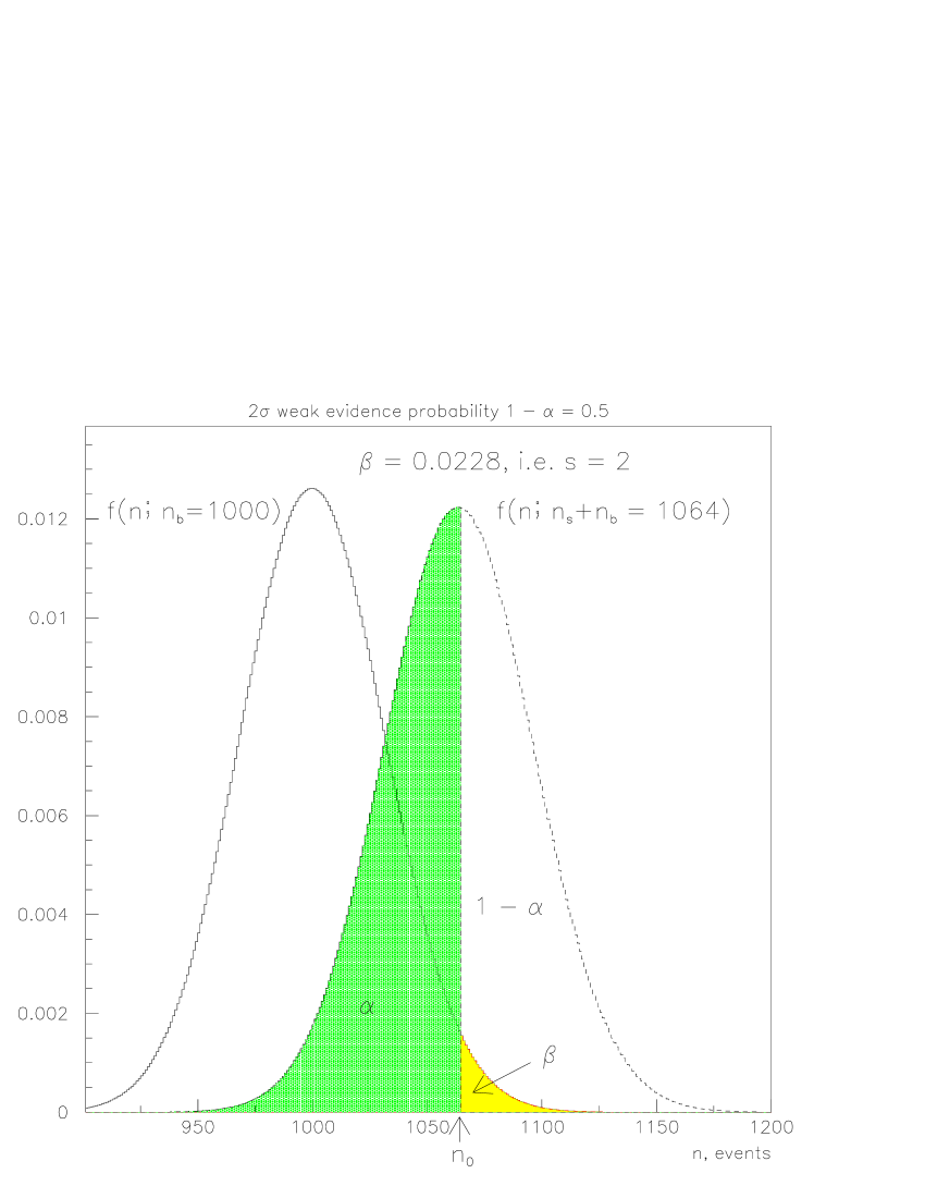
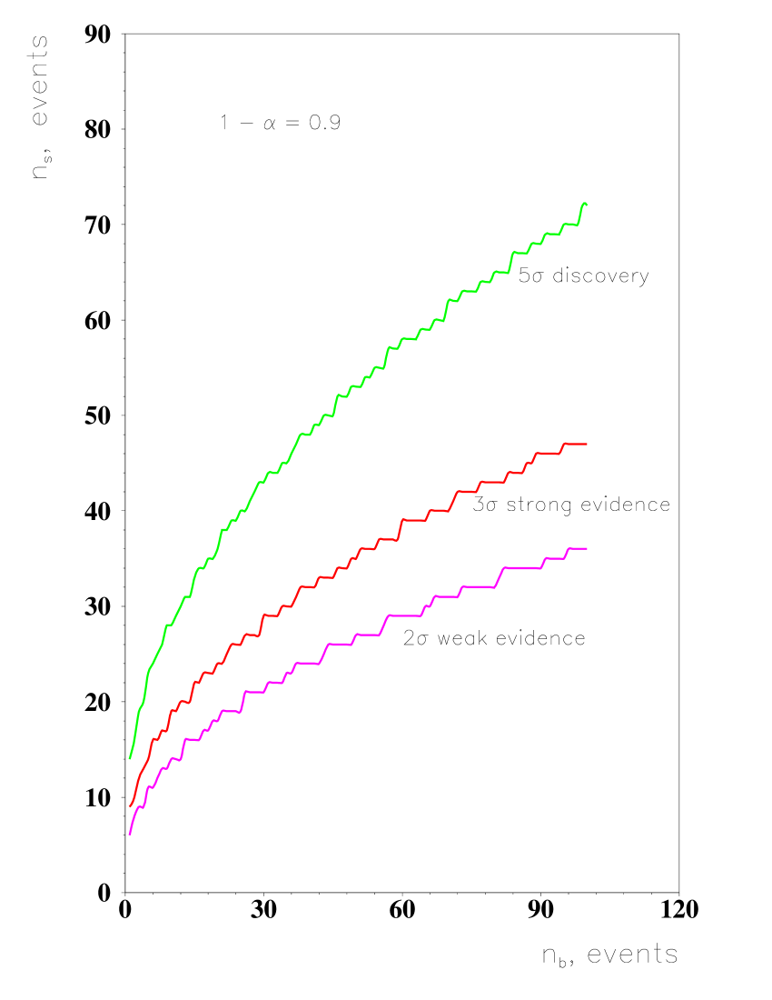
Figure 1: The case $n_{b}\gg 1$. Poisson distributions with parameters $\lambda=1000$ (left) and $\lambda=1064$ (right). Here $1-\alpha=0.5$ and $\beta=0.02275$ (i.e. $s=2$).

Figure 2: Dependences $n_{s}$ versus $n_{b}$ for $1-\alpha=0.9$ and for different values of $\beta$.

3 Effects of one sided systematic errors on the discovery potential

We consider here forthcoming experiments to search for new physics. In this case we must take into account the systematic uncertainty which has theoretical origin without any statistical properties. For example, two loop corrections for most reactions at present are not known. In principle, it is “reproducible inaccuracy introduced by faulty technique” [10] and according to [11] it contains the sense of “incompetence”. If the predicted number of background events strongly exceeds the predicted number of signal events the discovery potential is the sensitive to this uncertainty. In this case we can only estimate the scale of influence of background uncertainty on the observability of signal, i.e. we can point the admissible level of uncertainty in theoretical calculations for given experiment proposal.

Suppose uncertainty in the calculation of exact background cross section is determined by parameter $\delta$, i.e. the exact cross section lies in the interval $(\sigma_{b},\sigma_{b}(1+\delta))$ and the exact value of the average number of background events lies in the interval $(n_{b},n_{b}(1+\delta))$. Let us suppose $n_{b}\gg n_{s}$. As we know nothing about possible values of average number of background events, we consider the worst case [3]. Taking into account formulae (3) and (4) we have the formulae

$$\beta=\sum^{\infty}_{n=n_{0}+1}f(n;n_{b}(1+\delta))\leq\Delta$$ (5)

$$1-\alpha=\sum^{\infty}_{n=n_{0}+1}f(n;n_{b}+n_{s}).$$ (6)

Formulae (5,6) realize the worst case when the background cross section $\sigma_{b}(1+\delta)$ is the maximal one, but we think that both the signal and the background cross sections are minimal.

The example of using these formulae is shown in Fig.3. We see the sample of 200 (with, as expected, 100 background) events that will be enough to reach 90% probability of discovery with 25% systematic uncertainty of theoretical estimation of background.

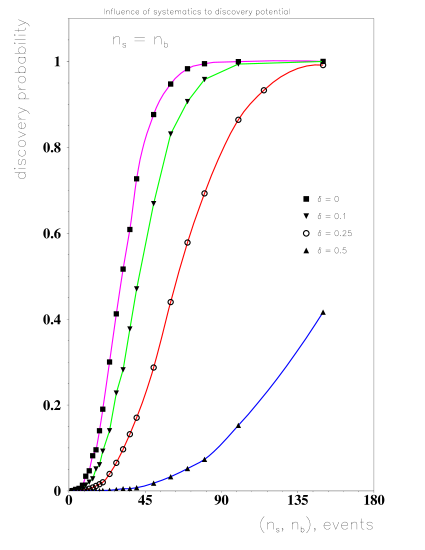
Figure 3: Discovery probability versus $n_{s}$ for different values of systematic uncertainty $\delta$ for the case $n_{s}=n_{b}$. The curves are constructed under condition $\beta=2.85\cdot 10^{-7}$.

4 An account of statistical uncertainty in the determination of $n_{s}$ and $n_{b}$

Usually, an experimentalist would extract the numbers $n_{s}$ and $n_{b}$ from a Monte Carlo simulation of the planned experiment, which results in the statistical errors. If the probability of true value of parameter of Poisson distribution (the conditional probability) to be equal to any value of $\lambda\geq 0$ in the case when one observation $n_{b}=\hat{n}$ or $n_{s}+n_{b}=\hat{n}$ is known we have to take into account the statistical uncertainties in the determination of these values.

Let us write down the density of Gamma distribution $\Gamma_{a,n+1}$ as

$$g_{n}(a,\lambda)=\displaystyle\frac{a^{n+1}}{\Gamma(n+1)}e^{-a\lambda}\lambda^{n},$$ (7)

where $a$ is a scale parameter, $n+1>0$ is a shape parameter, $\lambda>0$ is a random variable, and $\Gamma(n+1)=n~{}!$ is a Gamma function.

Let us set $a=1$, then for each $n$ a continuous function

$$g_{n}(\lambda)=\displaystyle\frac{\lambda^{n}}{n!}e^{-\lambda},~{}\lambda>0,~{}n>-1$$ (8)

is the density of Gamma distribution $\Gamma_{1,n+1}$ with the scale parameter $a=1$ (see Fig.4). The mean, mode, and variance of this distribution are given by $n+1,~{}n$, and $n+1$, respectively.

As it follows from the article [12] and is clearly seen from the identity [13] (Fig.5)

$$\sum_{n=\hat{n}+1}^{\infty}{f(n;\lambda_{1})}+\int_{\lambda_{1}}^{\lambda_{2}}{g_{\hat{n}}(\lambda)d\lambda}+\sum_{n=0}^{\hat{n}}{f(n;\lambda_{2})}=1~{},~{}~{}~{}i.e.$$ (9)

$\displaystyle\sum_{n=\hat{n}+1}^{\infty}{\frac{\lambda_{1}^{n}e^{-\lambda_{1}}}{n!}}+\int_{\lambda_{1}}^{\lambda_{2}}{\frac{\lambda^{\hat{n}}e^{-\lambda}}{\hat{n}!}d\lambda}+\sum_{n=0}^{\hat{n}}{\frac{\lambda_{2}^{n}e^{-\lambda_{2}}}{n!}}=1~{}$

for any $\lambda_{1}\geq 0$ and $\lambda_{2}\geq 0$, the probability of true value of parameter of Poisson distribution to be equal to the value of $\lambda$ in the case of one observation $\hat{n}$ has probability density of Gamma distribution $\Gamma_{1,1+\hat{n}}$. The equation (9) shows that we can mix Bayesian and frequentist probabilities in the given approach.

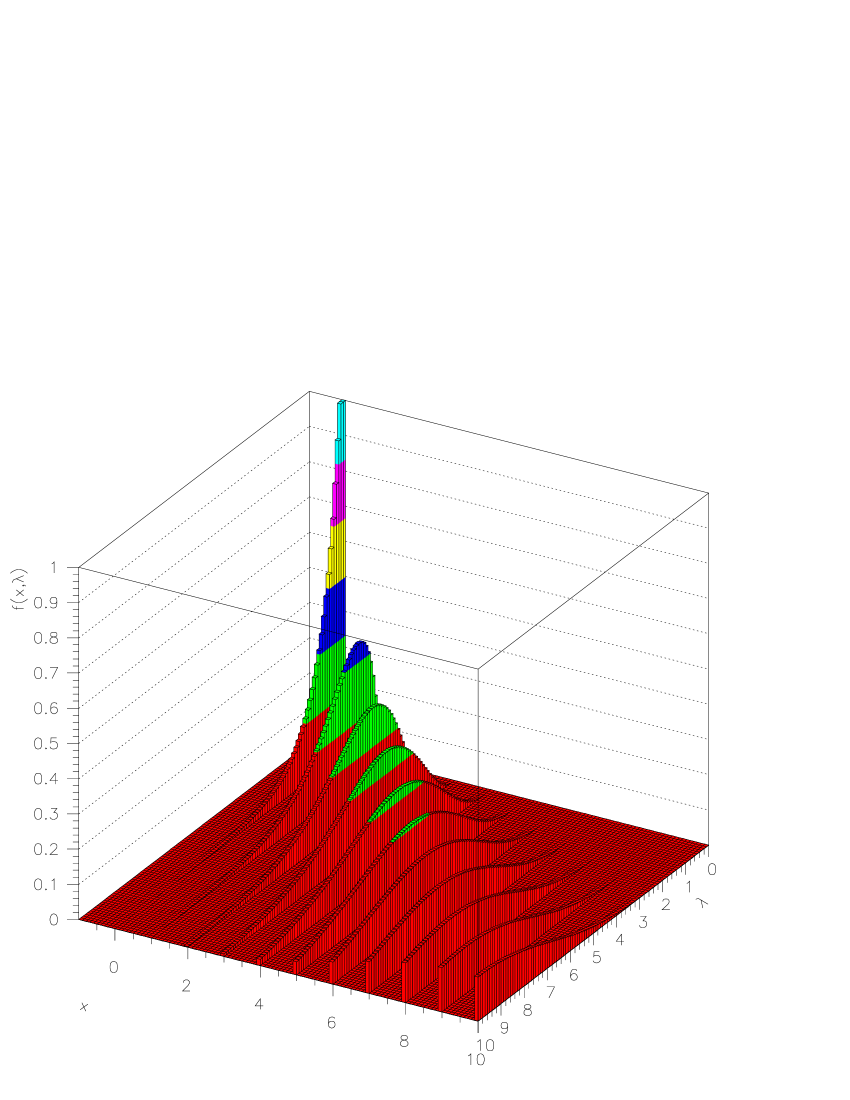
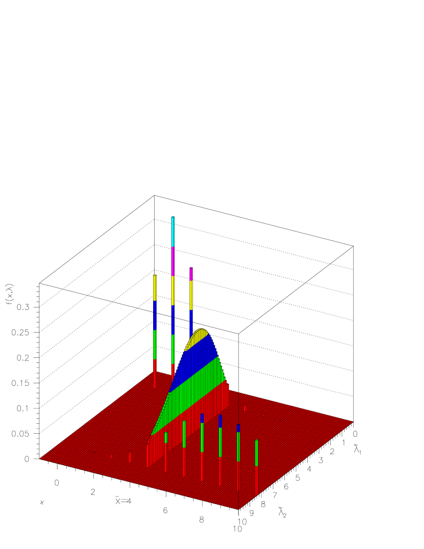
Figure 4: The behaviour of the probability density of the true value of parameter $\lambda$ for the Poisson distribution in case of $n$ observed events versus $\lambda$ and $n$. Here $f(n;\lambda)=g_{n}(\lambda)=\displaystyle\frac{\lambda^{n}}{n!}e^{-\lambda}$ is both the Poisson distribution with the parameter $\lambda$ along the axis $n$ and the Gamma distribution with a shape parameter $n+1$ and a scale parameter 1 along the axis $\lambda$.

Figure 5: The Poisson distributions $f(n,\lambda)$ for $\lambda$’s determined by the confidence limits $\hat{\lambda}_{1}=1.51$ and $\hat{\lambda}_{2}=8.36$ in case of the observed number of events $\hat{n}=4$ are shown. The probability density of Gamma distribution with a scale parameter $a=1$ and a shape parameter $n+1=\hat{n}+1=5$ is shown within this confidence interval.

It allows to transform the probability distributions $f(n;n_{s}+n_{b})$ and $f(n;n_{b})$ accordingly to calculate the probability of discovery [14]

$$1-\alpha=1-\int_{0}^{\infty}{g_{n_{s}+n_{b}}(\lambda)\sum_{n=0}^{n_{0}}f(n;\lambda)d\lambda}=1-\sum_{n=0}^{n_{0}}\frac{C^{n}_{n_{s}+n_{b}+n}}{2^{n_{s}+n_{b}+n+1}},$$ (10)

where the critical value $n_{0}$ under the future hypotheses testing about the observability is chosen so that the Type II error

$$\beta=\int_{0}^{\infty}{g_{n_{b}}(\lambda)\sum_{n=n_{0}+1}^{\infty}f(n;\lambda)d\lambda}=\sum_{n=n_{0}+1}^{\infty}\frac{C^{n}_{n_{b}+n}}{2^{n_{b}+n+1}}$$ (11)

could be less or equal to $2.85\cdot 10^{-7}$. Here $C^{n}_{N}$ is $\displaystyle\frac{N!}{n!(N-n)!}$. Also we suppose that the Monte Carlo luminosity is exactly the same as the data luminosity later in the experiment. The behaviour of discovery probability with and without account for this uncertainty is shown in Fig.6.

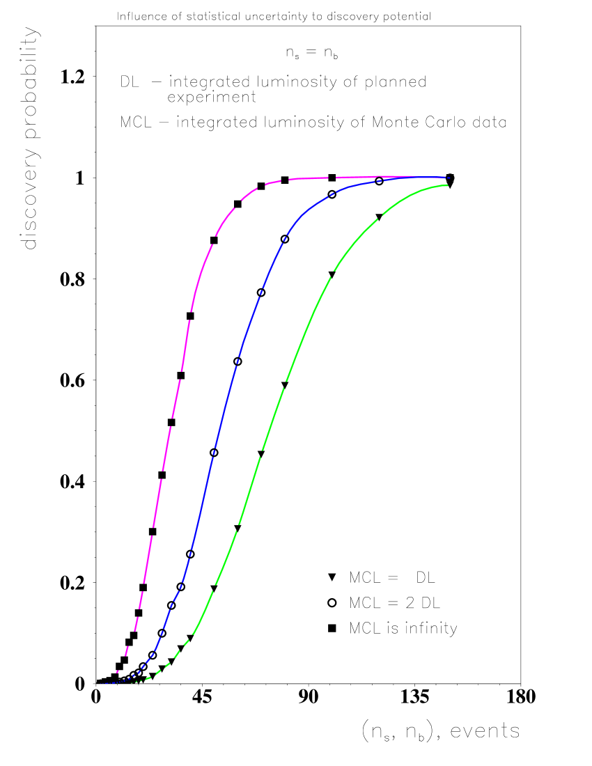
Figure 6: Discovery probability versus $n_{s}$ with and without account for statistical uncertainty in determination of $n_{s}$ and $n_{b}$. The case $n_{s}=n_{b}$. The curves are constructed under condition $\beta=2.85\cdot 10^{-7}$.

The Poisson distributed random values have a property: if $\xi_{i}\sim Pois(\lambda_{i}),~{}i=1,2,\dots,m$ then $\displaystyle\sum^{m}_{i=1}\xi_{i}\sim\displaystyle Pois(\sum^{m}_{i=1}\lambda_{i})$. It means that if we have $m$ observations $\hat{n}_{1}$, $\hat{n}_{2}$, $\dots$, $\hat{n}_{m}$ of the same random value $\xi\sim Pois(\lambda)$, we can consider these observations as one observation $\displaystyle\sum^{m}_{i=1}\hat{n}_{i}$ of the Poisson distributed random value with parameter $m\cdot\lambda$. According to eq.(9) the probability of true value of parameter of this Poisson distribution has probability density of Gamma distribution $\displaystyle\Gamma_{1,1+\sum_{i=1}^{m}{\hat{n}_{i}}}$. Using the scale parameter $m$ one can show that the probability of true value of parameter of Poisson distribution in the case of $m$ observations of the random value $\xi\sim Pois(\lambda)$ has probability density of Gamma distribution $\displaystyle\Gamma_{m,1+\sum_{i=1}^{m}{\hat{n}_{i}}}$, i.e. (see eq.7)

$$G(\sum{\hat{n}_{i}},m,\lambda)=g_{(\sum_{i=1}^{m}{\hat{n}_{i}})}(m,\lambda)=\displaystyle\frac{m^{(1+\sum_{i=1}^{m}{\hat{n}_{i}})}}{(\sum_{i=1}^{m}{\hat{n}_{i}})!}e^{-m\lambda}\lambda^{(\sum_{i=1}^{m}{\hat{n}_{i}})}.$$ (12)

Let us assume that the integrated luminosity of planned experiment is $L$ and the integrated luminosity of Monte Carlo data is $m\cdot L$. For instance, we can divide the Monte Carlo data into $m$ parts with luminosity corresponding to the planned experiment. The result of Monte Carlo experiment in this case looks as set of $m$ pairs of numbers $(~{}(n_{b})_{i},~{}(n_{b})_{i}+(n_{s})_{i}~{})$, where $(n_{b})_{i}$ and $(n_{s})_{i}$ are the numbers of background and signal events observed in each part of Monte Carlo data. Let us denote $\displaystyle N_{b}=\sum_{i=1}^{m}{(n_{b})_{i}}$ and $\displaystyle N_{s+b}=\sum_{i=1}^{m}{((n_{s})_{i}+(n_{b})_{i})}$. Correspondingly (see page 98, [7]),

$$\beta=\int_{0}^{\infty}{G(N_{b},m,\lambda)\sum_{n=n_{0}+1}^{\infty}f(n;\lambda)d\lambda}=\sum_{n=n_{0}+1}^{\infty}C^{n}_{N_{b}+n}\frac{m^{1+N_{b}}}{(m+1)^{1+N_{b}+n}}\leq\Delta,$$ (13)

$$1-\alpha=1-\int_{0}^{\infty}{G(N_{b+s},m,\lambda)\sum_{n=0}^{n_{0}}f(n;\lambda)d\lambda}=1-\sum_{n=0}^{n_{0}}C^{n}_{N_{s+b}+n}\frac{m^{1+N_{s+b}}}{(m+1)^{1+N_{s+b}+n}}.$$ (14)

As a result, we have a generalized system of equations for the case of different luminosity in planned data and Monte Carlo data. The set of values $\displaystyle C^{n}_{N+n}\frac{m^{1+N}}{(m+1)^{N+n+1}},~{}n=0,1,\dots$ is a negative binomial (Pascal) distribution with real parameters $N+1$ and $\displaystyle\frac{1}{m+1}$, mean value $\displaystyle\frac{1+N}{m}$ and variance $\displaystyle\frac{(1+m)(1+N)}{m^{2}}$.

5 Conclusions

In this paper we have described a method to estimate the discovery potential on new physics in planned experiments where only the average number of background $n_{b}$ and signal $n_{s}$ events is known. The “effective significance” $s$ of signal for given probability of observation is discussed. We also estimate the influence of systematic uncertainty related to non-exact knowledge of signal and background cross sections on the probability to discover new physics in planned experiments. An account of such kind of systematics is very essential in the search for supersymmetry and leads to an essential decrease in the probability to discover new physics in future experiments. The texts of programs can be found in http://home.cern.ch/bityukov. A method for account of statistical uncertainties in determination of mean numbers of signal and background events is proposed. Appendix A demonstrates the interrelation between Gamma- and Poisson distributions. The approach for estimation of exclusion limits on new physics is described in Appendix B.

The author is grateful to N.V. Krasnikov and V.F. Obraztsov for the interest and useful comments, S.S. Bityukov, Yu.P. Gouz, V.V. Smirnova, V.A. Taperechkina for fruitful discussions and E.A. Medvedeva for help in preparing the paper. The author thanks to referee of paper for the constructive criticism. This work has been supported by grant CERN-INTAS 00-0440.

Appendix A The interrelation between gamma- and Poisson distributions

The identity (9) (Fig.5)

$$\sum_{n=\hat{n}+1}^{\infty}{f(n;\lambda_{1})}+\int_{\lambda_{1}}^{\lambda_{2}}{g_{\hat{n}}(\lambda)d\lambda}+\sum_{n=0}^{\hat{n}}{f(n;\lambda_{2})}=1~{},$$

can be easy generalized, as an example , to

$$\sum_{n=k_{m}+1}^{\infty}{f(n;\lambda_{1})}+\sum^{m}_{i=1}[\int_{\lambda_{i}}^{\lambda_{i+1}}{g_{k_{m+1-i}}(\lambda)d\lambda}+\sum_{n=k_{m-i}+1}^{k_{m+1-i}}{f(n;\lambda_{i+1})}]$$

$$+f(k_{0};\lambda_{m+1})=1$$ (15)

for any real $\lambda_{i}\geq 0$, $i\in[1,m+1]$, integer $m>0$, $k_{l}>k_{l-1}\geq 0$, $l\in[1,m]$, $k_{0}=0$.

As a result of such type generalizations we have got

$$\int_{\lambda_{1}}^{\lambda_{2}}{g_{m}(\lambda)d\lambda}+\sum_{i=n+1}^{m}{f(i;\lambda_{2})}+\int_{\lambda_{2}}^{\lambda_{1}}{g_{n}(\lambda)d\lambda}-\sum_{i=n+1}^{m}{f(i;\lambda_{1})}=0~{},$$ (16)

i.e.

$\displaystyle\int_{\lambda_{1}}^{\lambda_{2}}{\frac{\lambda^{m}e^{-\lambda}}{m!}d\lambda}+\sum_{i=n+1}^{m}{\frac{\lambda_{2}^{i}e^{-\lambda_{2}}}{i!}}+\displaystyle\int_{\lambda_{2}}^{\lambda_{1}}{\frac{\lambda^{n}e^{-\lambda}}{n!}d\lambda}-\sum_{i=n+1}^{m}{\frac{\lambda_{1}^{i}e^{-\lambda_{1}}}{i!}}=0~{},$

for any real $\lambda_{1}\geq 0$, $\lambda_{2}\geq 0$, and integer $m>n\geq 0$.

Appendix B Exclusion limits [3, 4]

It is important to know the range in which a planned experiment can exclude presence of signal at given confidence level ($1-\epsilon$). It means that we will have uncertainty in future hypotheses testing about non-observation of signal which equals to or less than $\epsilon$. In refs.[17, 18] different methods to derive exclusion limits in prospective studies have been suggested.

We propose to use the relative uncertainty

$$\tilde{\kappa}=\displaystyle\frac{\alpha+\beta}{2-(\alpha+\beta)}$$ (17)

which will take place under hypotheses testing $H_{0}$ versus $H_{1}$. It is a probability of wrong decision. This probability $\tilde{\kappa}$ in case of applying the equal-probability test [4] is a minimal relative value of the number of wrong decisions in the future hypotheses testing for Poisson distributions. It is the uncertainty in the observability of the new phenomenon. Note that in this case the probability of correct decision $1-\tilde{\kappa}$ (the relative number of correct decisions) may be considered as a distance between two distributions (the measure of distinguishability of two Poisson processes) in frequentist sense. This distance changes from zero up to unity (as a result of the definition of equal-probability test).

References

- [1] Particle Data Group, D.E. Groom et al., Eur.Phys.J. C15 (2000) 1 (Section 28).
- [2] W.T. Eadie, D. Drijard, F.E. James, M. Roos, and B. Sadoulet, Statistical Methods in Experimental Physics, North Holland, Amsterdam, 1971.
- [3] S.I. Bityukov and N.V. Krasnikov, New physics discovery potential in future experiments, Modern Physics Letters A13(1998)3235.
- [4] S.I. Bityukov and N.V. Krasnikov, On the observability of a signal above background, Nucl.Instr.&Meth. A452 (2000) 518; S.I. Bityukov and N.V. Krasnikov, On observability of signal over background, Proceedings of Workshop on Confidence limits, YR, CERN-2000-005, 17-18 Jan., 2000, pp. 219-235, eds. F. James, L. Lyons, Y. Perrin.
- [5] P. Sinervo, Signal significance in particle physics, IPPP/02/39, DCPT/02/78, Proceedings of International Conference “Advanced Statistical Techniques in Particle Physics”, March 18-22, 2002, Durham, UK, p.64. http://www.ippp.dur.ac.uk/statistics/
- [6] T. Junk, Confidence level computation for combining searches with small statistics, Nucl.Instr.&Meth. A434 (1999) 435; V.F. Obraztsov, Confidence limits for processes with small statistics in several subchannels and with measurement errors, Nucl.Instr.&Meth. A316 (1992) 388; Erratum, Nucl.Instr.&Meth. A399 (1997) 500.
- [7] A.G. Frodesen, O. Skjeggestad, H. Tft, Probability and Statistics in Particle Physics, UNIVERSITETSFORLAGET, Bergen-Oslo-Troms, 1979, p.408.
- [8] I. Narsky, Estimation of Upper Limits Using a Poisson Statistic, Nucl.Instrum.Meth. A450 (2000) 444.
- [9] S.I. Bityukov, N.V. Krasnikov, Uncertainties and Discovery Potential in Planned Experiments, IPPP/02/39, DCPT/02/78, Proceedings of International Conference “Advanced Statistical Techniques in Particle Physics”, March 18-22, 2002, Durham, UK, p.77. http://www.ippp.dur.ac.uk/statistics/; e-Print: hep-ph/0204326, 2002.
- [10] R. Bevington, Data reduction and Analysis for the Physical Sciences, McGraw Hill 1969.
- [11] R. Barlow, Systematic errors: facts and fictions, IPPP/02/39, DCPT/02/78, Proceedings of International Conference “Advanced Statistical Techniques in Particle Physics”, March 18-22, 2002, Durham, UK, p.134. http://www.ippp.dur.ac.uk/statistics/
- [12] R.D. Cousins Why isn’t every physicist a Bayesian ? Am.J.Phys 63 (1995) 398-410.
- [13] S.I. Bityukov, N.V. Krasnikov, V.A. Taperechkina, Confidence intervals for Poisson distribution parameter, Preprint IFVE 2000-61, Protvino, 2000; also, e-Print: hep-ex/0108020, 2001.
- [14] S.I. Bityukov and N.V. Krasnikov, Some problems of statistical analysis in experiment proposals, Proceedings of CHEP’01 International Conference on Computing in High Energy and Nuclear Physics, September 3-7, 2001, Beijing, P.R. China, Ed. H.S. Chen, Science Press, Beijing New York, p.134. http://www.ihep.ac.cn/chep01/
- [15] B. Escoubes, S. De Unamuno and O. Helene, Experimental signs pointing to a Bayesian instead of a classical approach for experiments with a small number of events, Nucl.Instr.&Meth. A257 (1987) 346.
- [16] D. Silverman, Joint Bayesian Treatment of Poisson and Gaussian Experiments in a Chi-squared Statistic, e-Print: physics/9808004, 1998
- [17] J.J.Hernandez, S.Navas and P.Rebecchi, Estimating exclusion limits in prospective studies of searches, Nucl.Instr.Meth. A 378, 1996, p.301.
- [18] T.Tabarelli de Fatis and A.Tonazzo, Expectation values of exclusion limits in future experiments (Comment), Nucl.Instr.Meth. A403, 1998, p.151.