Exploring the Micro-Structure of the Proton:

from Form Factors to DVCS

John P. Ralston^a and Pankaj Jain^b

Abstract: For a long time people made the mistake of thinking the proton was understood. New experiments, ranging from form factors to deeply virtual Compton scattering, promise a new era of highly informative studies. Among the controversial topics of the future may be such basic features as the physical size of the proton, the role of quark orbital angular momentum, and the possibility of making ”femto-photographic” images of hadronic micro-structure.

Reflections on the First Form Factor

Apology: Hadronic physics is still something young. And yet, people thought they understood the proton for a long time. This was not right, but persisted because so little was known. When little is known, we cannot even find out what might be known.

Now we face a new time, an era promising informative measurements on how hadrons are made. We should stand back, and assess how hadronic physics came not to be understood up to this point. I apologize in advance for needing to explain things gone awry at an elementary level. I will review some history, from ancient to current day, to set the stage for new developments exploring the three-dimensional micro-structure of hadrons.

Rethinking the thinking about form factors led to the question: what was the first form factor? Newton gave us the gravitational form factor of the Earth. College students should repeat the integration exercise, assuming a uniform density. You cannot cheat and use Gauss’ Law, because Gauss was not yet born.

The claims about the form factor were probably met with some skepticism by the gentlemen of the Royal Society. First, the form factor describes an incredibly unnatural theory with an exceedingly small and arbitrary parameter. The theory explained little new in terms of phenomena: things falling to the Earth being already known. The main parameter was made absurdly small to escape from direct observation of the claimed universal force. Then there had to be absurdly large parameters, such as the mass of the Sun, to compensate the small parameter. The theory’s author sidestepped direct tests, and based results on astronomical data…and we all know how unreliable that kind of data can be! Following indirect arguments, and inventing private mathematical methods to justify it, Newton claimed that the entire Earth form factor could just be considered “the same as a point mass at the center”, a perfectly incredible result.

While the form factor acted like a point mass, nobody of course believed that the Earth was a point mass.

Cavendish was a hard-minded, bitter experimentalist who could go out and make the measurements that Newton shirked. The “Honorabilus Henricus Cavendish” enrolled at Peterhouse College of Cambridge at age 18 in 1749. He spent years on the Form Factor problem. Henry needed the Form Factor in the measurement of gravity from mountains. He chose a special hill, “Schieshallion”, because of its near conical form and calculability. The story that Cavendish “weighed the Earth” is only partly correct. Cavendish must have had a pretty good idea of the size of Newton’s $G$ from the start. Just equate $g=9.8m/s^{2}$ with $GM_{E}/R^{2}$. The Earth’s mass $M_{E}$ is estimated to be $4\pi R^{3}\rho/3$, where $\rho$ is the local density of rocks, something like 2-3 times the density of water. So Henry had $G\sim 3g/(4\pi R\rho)$ before he ever started his experiment. When Henry got an answer for $G$ several times larger, he did not believe it was anything fundamental. In experimental tradition, he complicated the form factor rather than challenge the theory. Now we say to “go to larger momentum transfer where there will be a dense core”. More than 200 years later this speculation remains untested by direct means. Seismology is very indirect, and what lies inside the Earth remains mysterious, although we may someday look inside with neutrino tomography [1].

The modern era produced the form factors of hadrons. People say that Rutherford postulated the central nucleus by looking at his data. Reading the actual paper [2] is very enlightening. One learns there was already an excuse for large scattering angles, coming from J. J. Thompson invoking multiple scattering in the plumb-pudding model. Rutherford’s paper is phenomenological, referring to data of Geiger and Marsden: he demolishes the proposal of multiple scattering on statistical grounds [2]. When Rutherford proposes the nuclear center, he was perhaps not the first, citing “…it is of interest that Nagoaka (Phil Mag vii, 441(1904)) has mathematically considered a ‘Saturnian atom’ (with ) …rings of electrons”. Predictably, there is a damaging typographic error, and it is right in the famous Rutherford formula for scattering!

Anyway, by 1929 the finite size of the strongly interacting nucleus was known. At the Royal Society in London, Rutherford stated [3] “It will be seen that this (data) makes the nucleus of Uranium very small, about $7\times 10^{-13}cm$…it sounds incredible but it may not be impossible”. Of course the hyperfine splittings of atomic physics gave similar numbers, and Yukawa knew it to predict his mesons.

In other words, everybody knew that the proton had a finite size for a long time. The “size” was hardly open to much question.

0.1 Recent Prehistory: Electron Beams

Our era is dominated by Robert Hofstadter’s spectacular measurements of the proton form factors via electron scattering. The two form factors are called $F_{1}$, $F_{2}$ and defined by

$$<p^{\prime},\,s^{\prime}|J^{\mu}|p,\,s>=\bar{u}(p^{\prime},\,s^{\prime})\ [\gamma^{\mu}F_{1}(Q^{2})+\frac{\kappa}{2M}F_{2}(Q^{2})\sigma^{\mu\nu}Q_{\nu}\ ]u(p,\,s).$$ (1)

Here $Q^{2}$ is the momentum transfer-squared; it is spacelike (negative) in electron scattering. One famous Hofstadter electron beam used the heroic energy of 188 MeV. Nobody faulted Hofstadter’s data [4], as far as I know, and the Nobel Prize of 1961 seems perfectly appropriate. But Robert already had the charge radius and its interpretation before he started his experiment.

Meanwhile there were serious questions about this specific interpretation of the form factors. I am summarizing all this history just to bring out these interpretation problems which persist today. The question is whether the low $Q$ form factors measure the Fourier transforms of charge and magnetic moment distributions. As far as I can tell, people with savvy backed away from this in the old days, yet many believe it today. The interpretation might be justified: I just don’t find credible justification for what has become an important point.

The influential book of Drell and Zachariasen [5] said “it is convenient to define” densities by Fourier transform in the Breit frame, following this by “…this definition depends on a particular definition of Lorentz frame in which the proton is not stationary, and therefore the relation of these densities to any real physical extent of the proton is quite unclear”. (It is also puzzling that the Breit frame $Q^{\mu}=(0,\,0,\,0,\,Q_{3})$ is very far from unique, and you will get the very same photon momentum with two sideways Lorentz boosts of arbitrary rapidity.) The target’s “mean-square radius” was stated to be “just measuring the slope of the form factor as $Q^{2}\rightarrow 0$.” This is a definition and meaningless. Sakurai’s book [6] shows that the form factors could be reproduced by the claimed static distributions, without saying that such static distributions had been measured. Other books (e.g. Schweber [7]) are very terse, avoiding interpretation.

Apparently people became divided, between those accepting the form factors were Fourier tranforms of real spatial distributions, and those who found this misleading. An important review article by Yennie, Levy and Ravenhall [8] was unequivocal, stating:

Objection 1: “The essential point is that measurement of structure within a distance $d$ requires values of $|\vec{Q}|$ of order $1/d$…

and going on to say:

Objection 2:…and if absorption of this momentum causes recoil (i.e if $|\vec{Q}|>Mc/\hbar$) the intuitive concepts of static charge and current distributions are no longer valid.”

The labels of Objection 1 and Objection 2 are my own. Yennie doubly rejected the identification of form-factor as charge density. Indeed the Appendix of Yennie’s important 1959 Reviews of Modern Physics [8] lists two other form factors denoted $A$ and $B$, now called $G_{M}$ and $G_{E}$, which are linear combinations of Rosenbluth’s:

$$G_{M}=F_{1}+\kappa F_{2};$$ (2)

$$G_{E}=F_{1}+\kappa\tau F_{2};\>\>\tau=\frac{Q^{2}}{4m_{p}^{2}}.$$ (3)

(Sachs cites this when he writes his own article: perhaps Yennie et al found the Sachs form factors first.) Yennie et al gave the alternative linear combinations just to emphasize that the connection of form factor and charge density was highly arbitrary. A few years later [9], Yennie reiterated his stance, adding that “…Sachs and collaborators do hold there is a real physical meaning” to the Fourier transform relation. Reading Sachs’ paper [10] gives little clue why Sachs was so vehement in the claim, or why people believed it.

Objection 2 is not a worry if the momentum transfer is small compared to the mass. This seems to have diverted attention. Meanwhile Objection 1, which is the objection of optical resolution and indeed the entire problem of dynamics, is swept under the rug!

Right on the heels of the Hofstadter data, dynamics forced the interpretation in terms of VMD, vector meson dominance. The isoscalar and isovector mesons were predicted [11] by saturating the photon exchange with mesons. Physically, VMD means that the meson strongly polarizes the proton by resonant pion exchanges, which then re-interact by resonant pion exchanges. What scrap of the proton left over …that is not the meson…is not even part of the model!

How then is the “charge radius” related to the undisturbed radius of the proton? Throwing pillows at a baseball, do you measure the size of the baseball or the size of the pillows? The “most general possible” nature of the Rosenbluth formula subconsciously convinced many that the question did not matter. Hyperfine and Lamb shift experiments use the same matrix element, so there is nothing but trivial consistency there.

Yet Objection 1 was really about optics. Following Yennie, it is hard to believe that a momentum transfer of 200 MeV could give anything else but a distance scale of 1 Fm. The measurement of 200 MeV put in a Fermi scale and came out with a Fermi scale. In what sense was the size of the proton measured?

Since the process is dynamical, I arrived at an idea that perhaps some of the “pion cloud” is actually stirred up by the strong interaction itself, and was not there in the proton to start with. In fact, dynamical strong polarization effects do occur for atoms on metal surfaces, where measured dipole moments per charge can be thousands of times larger than the physical size of the atoms. It is explained by fast electrons free to move quickly on the surfaces. In the 1960’s nobody had a clue that there existed light, relativistic quarks, but now we know these quarks exist, and they react on time scales much faster than an inverse 200 MeV.

Yet the idea of an intrinsic 1 Fm pion cloud around nucleons is deeply ingrained. It takes effort and initiative to question what we may or may not know about it. Everyone knows that a static system coupled to a meson of mass $\mu$ uses a Green function $1/(\vec{k}^{2}+\mu^{2})$ and cannot fall off with distance less rapidly than $e^{-\mu r}$. This says nothing about all the rest of the interior and dynamical structure, for which optical resolution much better than $1/\mu$ is required to say anything.

Imagine how interesting it would be if the undisturbed size–the quark radius of the proton – is not the same as the so-called charge radius measured via VMD. This would be a gold mine, not only for what the proton is. It would be a gold-mine of classic scientific controls. When distinct things can be compared, the standard measurements called the charge radii become that much more valuable and interesting. And so the beautiful experimental accomplishments of the neutron charge radius [12], for instance, would not just be isolated marvels but would be something to compare and to teach us more. One needs large $Q^{2}$, of course, to pursue this.

We then move to the modern description of large $Q^{2}$ form factors. Unfortunately the topic has little to do with the bulk of the Fock space components making up the proton. However we will return to probing the overall makeup of the proton afterwards.

1 Hadronic Form Factors at Large $Q^{2}$

Our approach to large $Q^{2}$ form factors in pQCD uses impact parameter factorization [13, 14]. In this scheme the transverse spatial separation $\vec{b}$ between quarks, as well as the longitudinal momentum fraction $x$, is used to describe amplitudes. The impulse approximation, which we consider the hallmark of pQCD, is used to separate a hard-scattering kernel from wave functions (or more general correlations) with longer time-scales. In the impulse approximation the $k^{-}$ integrations are done to evaluate products at light-cone time zero. The expression for a baryon form-factor $F$ scattering 3 quarks takes the form

$$F(Q^{2})=\int d^{2}b_{1}d^{2}b_{2}dx_{1}\ldots dx_{4}\bar{\psi}(x_{i},\,\vec{b}_{i};\,Q)H(Q,\,x_{i},\,\vec{b}_{i})\psi(x_{i},\,\vec{b}_{i};\,Q).$$ (4)

Note the following:

$\bullet$ This method does not make prior assumptions about short distance. Current research in pQCD has found that the assumption that all $b_{i}\rightarrow 0$ is neither justified nor necessary.

Theorists started with $b\rightarrow 0$. However the old “operator product expansion” (OPE) was shown unable to account for numerous physically observable effects, such as the Sudakov corrections [15, 16]. In Eq. 4 the Sudakov effects are merged into definitions of the wave functions: elsewhere [15, 16, 17] they are denoted $e^{-S(x_{i},\,\vec{b}_{i};\,Q)}.$

$\bullet$ The method explains the constantly observed phenomena [18] known as hadronic helicity flip, in which the sums of the helicities of the hadrons going into the reaction does not equal the sum of those going out. For a while people had the impression helicity flip was not part of pQCD: it is, in fact, a mainstream part, and quantitative calculations of hadronic helicity flip in pQCD are in the literature [19]. The cause for misunderstanding is over-reliance on $b\rightarrow 0$ in quick asymptotic estimates.

$\bullet$ Quark-counting must play a role, as originally envisioned by Brodsky and Farrar and Matveev et al [20]. Under this hypothesis, and as confirmed by perturbation theory, the addition of extra quanta beyond the valence contains important regions that produce suppression at large $Q$. The topic has been controversial, and “‘strongly polarized”, but the power-law scaling observed in so much data is not to be dismissed: the data exists despite many theoretical complaints [21].

Yet we avoid the later asymptotic short distance (ASD) approach of Brodsky and Lepage [22] sometimes said to be the same thing as QCD. It is not the same thing. The ASD formalism is decisively ruled out by observing hadronic helicity flip…and ruled out many times. In particular, $F_{2}=0$ in the ASD formalism for massless quarks in valence state. Hadron helicity violation is too universal and $F_{2}$ is too large to be explained by flipping the spins with perturbative quark masses $\sim$ few MeV: so drop ASD.

$\bullet$ The impact-parameter coordinate has been around since the beginning of time. Our usage was influenced by the Sterman and Botts [13] treatment of the Landshoff independent scattering processes of $pp$ elastic scattering. Independent scattering is yet another example of something beyond the capacity of the ASD formalism. Impact-parameter factorization also allows the systematic pQCD description of color transparency [14, 23] and nuclear filtering [24] which are beyond ASD. Subsequent to our treatment of nuclear form factor transparency [14], it was realized that free space hadron form factors needed the impact parameter factorization, too [15, 16].

By similar care, the helicity flip terms are also saved for evaluation in pQCD [19]. Helicity flip calculations are “leading twist” for what they describe. It is grossly misleading to compare them to “higher twist” meaning the subleading corrections to other matrix elements with different transformation properties. This is why the approach of Eq. 4 constitutes a different and more general theory of hadron scattering than the asymptotic short distance one. By now most groups studying quark-counting use the impact parameter factorization.

1.1 Quark Orbital Angular Momentum

A compelling motivation for using impact parameter coordinates is that it allows classification of wave functions in orbital angular momentum.

The quantization $z$-axis is along the direction of particle momentum. The natural orbital angular momentum of high energy processes uses the Lorentz-invariant subgroup SO(2) of rotations about the z-axis. We do not discuss SO(3) representations, which do not transform well. The representations of SO(2) orbital angular momentum (OAM) are labeled by an integer $m$, the eigenvalue of an operator $L_{z}.$ The expansion of wave functions in OAM is conventionally written

$$\psi(x_{i},\,\vec{b}_{i};\,Q)=\sum_{m}e^{im\phi}\psi_{m}(x_{i},\,|\vec{b}_{i}|;\,Q).$$

On general grounds of continuity, the expansion coefficients $\psi_{m}(x_{i},\,|\vec{b}_{i}|;\,Q)$ obey a power rule,

$$\lim_{b\rightarrow 0}\,\psi_{m}(x_{i},\,|\vec{b}_{i}|;\,Q)\sim b^{|m|}.$$ (5)

We call this the “$b^{m}$ rule”. If a model takes the limit $b\rightarrow 0$ in the first step, only $m=0$ survives, and all information about quark OAM is forever lost. Historically this faulty limiting procedure [22] underlies the misconception that hadron helicity flip could not be treated straightforwardly in pQCD.

Despite popular belief, there is no power-counting preference for high-energy wave functions to be in the $m=0$ “s-wave”. For a simple example, consider the $q\bar{q}$ Bethe-Salpeter wave function $\psi_{\pi}$ for a pion of momentum $p$. There are four invariant wave functions:

$$\psi_{\pi}=Ap\hskip-5.03125pt\hbox to5.03125pt{\hss\sl/\/\hss}\gamma_{5}+B[p\hskip-5.03125pt\hbox to5.03125pt{\hss\sl/\/\hss},\,b\hskip-4.29166pt\hbox to4.29166pt{\hss\sl/\/\hss}]\gamma_{5}+Cb\hskip-4.29166pt\hbox to4.29166pt{\hss\sl/\/\hss}\gamma_{5}+D\gamma_{5}$$ (6)

The first two terms (A, B) scale equally like $p$ in the high energy limit, representing the “large” components of the quark operators. Indeed scaling like $p$ is the largest possible result one can get from two Dirac spinor field operators. Note that $B$ carrys $L_{z}=\pm 1$, as seen by expanding $\vec{b}_{T}=b_{x}\pm ib_{y}$. So orbital angular momentum shows up in the transverse plane. By angular momentum counting, $L_{z}=\pm 1$ is the maximum for the pion ($|L_{z}|<2$ for the proton). The explicit factors of $b$ in Eq. 6 obey the $b^{m}$ rule, and the series expansions of coefficient functions $A,\,B,\,\ldots$ start at $b^{0}$ unless a model has extra selection rules. There are also small terms, namely $C$ and $D$, suppressed by $1/p$ in comparison. Vector mesons and baryons are described similarly: it is a nice exercise to find the eight (8) covariant wave functions of a vector meson [19].

How can one test directly if mesons contain quark OAM? We suggest nuclear filtering for $A>>1$ in the reactions of $\gamma^{*}(Q)+A\rightarrow meson+A^{*}$ [25]. The meson should carry all of the virtual photon energy $\nu$ up to resolution. The final nucleus $A^{*}$ can be disrupted, and the reaction need only be exclusive to the extent no extra pions escape. For $Q^{2}>{\rm GeV}^{2}$ this reaction involves sizable momentum transfer to the struck nucleon. The “big fat” $m\neq 0$ wave functions should be relatively depleted by filtering [24] compared to lean and mean $m=0$ types. To be specific, the leading short-distance vector mesons are longitudinal, so that the ratio $\sigma_{L}/\sigma_{T}$ should increase with increasing $A$ and fixed $Q^{2},\,\nu$. Everything we have learned from color transparency [24] says this filtering effect will be much more dramatic than the corresponding transparency effect of increased $\sigma_{L}/\sigma_{T}$ with fixed $A$ and increasing $Q^{2},\,\nu$. Indeed, small $A\sim 10$ is not nearly as good as large $A$, because small $A$ is dominated by edge effects.

Why do we not get the OAM wave functions by making a Lorentz boost? The boost operator in field theory is exponentially complicated in the Poincare generators: it creates interacting particles. The fact remains that our conventions are Lorentz invariant, and Gell-Mann’s quark model stands to be ruled out if quarks in the boosted proton have a lot of orbital angular momentum.

1.2 $F_{2}$ and Quark Orbital Angular Momentum

The most interesting example of usage is surely $F_{2}$. After seeing the data of Jones et al [26], which seemed to indicate previous concept errors in the treatment of $F_{2}$, we returned to predict that the ratio $QF_{2}/F_{1}$ should be constant [27, 28]. The subsequent measurements of Gayouet al [29] found a ratio $QF_{2}/F_{1}$ spectacularly constant, sparking enormous new interest in the subject. It appears that $QF_{2}/F_{1}$ is a scientifically pivotal quantity that will be important for years to come. We now explain our predictions and recent work.

Counting angular momentum as helicity in the high energy limit, the chirality flip of $F_{2}$ also causes one unit of physical angular momentum flip with corrections of order $m_{p}/Q$, where $m_{p}$ is the proton mass. Angular momentum conservation is maintained by the virtual photon breaking the symmetry in a frame where $Q^{\mu}=(0,\,\vec{Q}_{T}=\sqrt{-Q^{2}},\,0)$. Now it is inconsistent with the chiral symmetry of pQCD to allow a light quark (mass $m_{q}$) to flip helicity (with corrections of order $m_{q}/Q=5{\rm MeV}/Q$). It follows that there is a general $\delta L_{z}=\pm 1$ rule for the net quark orbital angular momentum change in the process. For very general reasons, then, we claim that $QF_{2}/F_{1}$ measures the strength of quark orbital angular momentum. [27, 28]. We believe this will be dominated by the $m=0,\,m=\pm 1$ OAM interference terms.

The facts of OAM of course tie directly to the proton’s “spin crisis”, which is replayed with every hadronic helicity flip deja vu all over again.

$F_{2}$ and the Moments of Hard Scattering Kernels

Elsewhere we discussed $F_{2}$ in several ways: first from an early, independent invention of generalized parton distributions [30] (apologies to Dittes et al [31] of whom we were unaware), then from wave function [27] and updated generalized parton distribution (GPD) points of view [28]. In the current work [32], we estimate $F_{2}$ using the kernel and wave-function re-arrangements of Sterman and Li [15]. The kernels are the 48 full, complicated Feynman diagrams evaluated to leading order in Fermion transverse momentum. After transforming to $b$ space (two integrals) there are four $x$ integrations left. We use the COZ distribution amplitudes [33] as a model for the $x$ dependence, and the full Sudakov kernel; parameters and formulas are given in Ref. [17, 16]. Examination of the Dirac algebra shows no selection rules preventing the claimed interference. We estimated $QF_{2}/F_{1}$ by calculating the moments of $b$ inside the integrands, because it is particularly important to see if $b\rightarrow 0$ is or is not an outcome of the calculation. The moments are defined by

$$\frac{QF_{2}}{F_{1}}\sim\frac{<b^{m}>}{<b^{0}>};$$

$$<b^{m}>=\int d^{2}b_{1}d^{2}b_{2}\>\>b^{m}\>\>dx_{1}\ldots dx_{4}\bar{\psi}(x_{i},\,\vec{b}_{i}\,Q)H(Q,\,x_{i},\,\vec{b}_{i})\psi(x_{i},\,\vec{b}_{i};\,Q).$$

(7)

In this intimidating expression we have tried to leave extra space to show that the ratio is simply the moment of $b^{m}$ divided by the moment of $1=b^{0}$.

We use the same hard scattering kernels discussed for years for $F_{1}$ and keeping all the diagrams of pQCD. By using Eq. 7 we have assumed that the $x$ dependence of non-zero OAM is close enough to standard models to make a reasonable estimate. The calculation tests whether there is any kinematic and power-related suppression of OAM at laboratory values of $Q^{2}.$ The kernels $H$ contain two factors of $K(x_{i}x_{j}\sqrt{Q^{2}b_{k}^{2}})$, modified Bessel functions, and are given in the literature [17, 16]. The previous thinking in the field was that if $Q^{2}\rightarrow\infty$ in the first step, we would get $<b^{m}>\sim 1/Q^{m}$. That step would be an asymptotic estimate, exactly of the kind subject to the ASD limit interchange problems discussed earlier, and we do not do it. Instead we first calculate the integrals and then look at the limit.

The result is shown in Fig. 1. The figure shows that $QF_{2}/F_{1}$ is supposed to be flat. Certainly one moment is nearly flat across the range of $Q^{2}$ accessible to existing and future experiments. We use the notation of Ref. [16]. The two $up$ quarks are labelled as quark 1 and 2 and the $down$ quark is labelled as quark 3. The coordinate system is chosen such that the quark 3 lies at the origin. Let ${\vec{B}_{1}}$, ${\vec{B}_{2}}$, ${\vec{B}_{3}}$ be the transverse positions of quark 1, 2 and 3 respectively. Then we define the transverse separations $b_{1}$, $b_{2}$ and $b_{3}$ by the relations, $b_{1}=|{\vec{B}_{1}}-{\vec{B}_{3}}|=|{\vec{B}_{1}}|$, $b_{2}=|{\vec{B}_{2}}-{\vec{B}_{3}}|=|{\vec{B}_{2}}|$ and $b_{3}=|{\vec{B}_{1}}-{\vec{B}_{2}}|$. In Fig. 1 we have plotted the moment of the transverse separations $b_{1}$ and $b_{2}$. We see that the moment $<b_{2}>$ is almost flat. The moment $<b_{1}>$ scales differently: this is perfectly reasonable, because the 3 quark integration has regions that are not symmetric. Since our approach is very general, we believe that the experiments finding $QF_{2}/F_{1}$ flat are seeing quark orbital angular momentum in a very definitive way. From the normalization of $QF_{2}/F_{1}$, the $m\neq 0$ wave functions must be normalized to a substantial fraction of the proton’s spin, in accord with our earlier observations [30, 28] and other work [34].

Figure 1: The moments $<b_{1}>$ (dashed line) and $<b_{2}>$ (solid line), as defined in the text, using the COZ distribution amplitude. We see that the moment $<b_{2}>$ is almost flat in contradiction to the ASD expectations.

What does the constituent quark model say in this regard? We refer readers to a growing literature. Frank and Miller [35] also predicted $QF_{2}/F_{1}\sim constant$ in 1994 on the basis of an earlier model of Schlupf [36]. The prediction has recently been updated and re-examined [37]. This model uses quark masses of about $260$ MeV, and focuses on care in respecting relativistic spin-projections. The spin-projections are the key because in the end the model predicts non-zero OAM on the light-cone, in remarkable concord with our much different starting point. Weber and collaborators [38] communicated results of much the same kind at this meeting.

GPD’s are also a good approach to the form factors, and a way to use both constituent quark-model and short-distance concepts. Afanasev’s [39] pretty calculation inspired Stoler [40], who has shown that the data for $F_{1},\,F_{2}$ can be fit in the GPD formalism up to 30 GeV². The starting point of this model does not show the relation to OAM, but it is contained in the references. Stoler shows that the data at the higher $Q^{2}$ regime requires a hard wave function in GPD terminology, or a hard scattering kernel in our language, or some original quark-counting (not ASD) contribution in any language. The results puts to rest claims [21, 41] that form factors are totally dominated by soft effects. In regard to GPD, we reiterate that there exists an infinite number of factorization methods, of which the GPD are one example: all are capable of representing pQCD, and it is not helpful for any one method or the other to claim to be “the unique” pQCD prediction.

How can one test directly if the mysterious ratio $QF_{2}/F_{1}\sim const$ is due to quark OAM? Use polarization transfer in heavy nuclei, $\vec{e}+A\rightarrow\vec{p}+A^{*}-1.$ It is a beautiful observable and an experiment on Oxygen has already shown it to be feasible at several GeV [42]. Again one needs nuclear filtering with nuclear number $A>>1$ to make any headway. $A>>1$ means Gold, not Carbon, and the door is open here. If not keep hammering. Filtering should deplete the “fatter” $m\neq 0$ components of the wave function relative to the $m=0$ component. The polarization ratio corresponding to $G_{E}/G_{M}$ should dramatically approach the ASD predictions for $A>>1$. In other words, $QF_{2}/F_{1}$ will drastically decrease with large $A$ and large $Q^{2}$: the rate of decrease can tell us something about the orbital configurations, with $|m|=2$ producing a faster decrease than $|m|=1$.

2 Beyond Form Factors: The $DVCS$ Microscope

The interpretation of form factors at low $Q^{2}$ being soft, theorists long requested large momentum transfer. Yet large $Q^{2}$ form factors, however fascinating, have very little to do with the undisturbed proton. In any Lorentz frame, and in any model, the proton is violently accelerated, and only a very tiny fraction of wave function is involved in the final outcome.

However there happens to be two kinds of momentum transfer in reactions with a virtual photon. Let $Q^{2}$ consistently denote the virtuality of the photon, its 4-momentum-squared. Let $t=(p-p^{\prime})^{2}$ denote the momentum transfer to the target. In form factors the kinematics is restricted to $Q^{2}=t$.

Meanwhile $Q^{2}\neq t$ in many reactions assuming that the momentum sent in by the virtual photon escapes by some other path. The most beautiful case is deeply virtual Compton scattering, (DVCS) describing $\gamma^{*}+p\rightarrow\gamma_{p^{\prime}}$, where $p,p^{\prime}$ denote hadron momenta. Up to a kinematic $t_{min}$ restriction (and $t_{min}$ goes close to zero for multi-GeV energies), reactions can have $|Q^{2}|>{\rm GeV}^{2}$ with $t_{min}\sim 0<|t|<{\rm GeV}^{2}$ in the laboratory. Much the same kinematics apply to virtual meson production, in which $\gamma^{*}$ is effectively converted to a meson such as a pion, rho or phi.

DVCS has caused a great deal of excitement because these reactions involve GPD’s. Moreover, GPD’s are diagonal in good coordinate bases, namely the impact parameter representation, allowing a probability interpretation [43, 27, 44]. However most studies had to assume that a GPD model would be (1) guessed by theory, (2) integrated with the quark and gluon kernels, (3) weighted by the quark and gluon couplings, and finally (4) lead to an observed cross section all mixed together. This is alarmingly indirect. I do not believe that GPD’s and many of the concepts used in GPD’s, are physically observable.

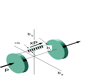
Figure 2: Cartoon of the natural interpretation of $GPD$. The fast struck quark (stack of plane waves) is located at the transverse offset position $\bar{b}_{T}$, while being spatially localized to within order $1/Q$ in the transverse directions. The quark’s longitudinal coordinate is not so well localized, but is spread along the light-cone in the direction conjugate to $xP$.

If we think about the reaction physically, the situation is remarkable [45]. The electron beam goes right through the proton (Fig 2) and radiates the detected photon almost instantly. First, the GPD is not observable, while the DVCS amplitude is physically observable. We should base our thinking on what is observable. The reason that an amplitude is observable, for once, is that the Bethe-Heitler interference term is large. This is good, because amplitudes contain complete physical information. It is possible to classify all the amplitudes and their scaling properties on the basis of angular momentum counting, again assuming that the quark helicity is conserved. On this basis it was predicted [46] that the spin and charge azimuthal asymmetries of DVCS would go like $sin(\phi)$ and $cos(\phi)$. The general series contains terms including $sin(\phi),\,sin(2\phi)$ (spin) and, $cos(\phi),cos(2\phi)$ (charge) and is extremely complicated but we made a list. The simple $sin(\phi)$ and $cos(\phi)$ distributions were actually observed [47], with very little room for higher harmonics. This is a amazingly beautiful confirmation of leading order pQCD in the handbag model. I must assume that scaling in $Q^{2}$ will be observed: it is important and necessary as a test of leading order pQCD. Meanwhile the situation seems very much like the observation of $\sigma_{L}/\sigma_{T}<<1$ in deeply inelastic scattering: the data is right on the verge of a breakthrough.

Since the amplitude is what is observable, we should think about how much information a complete amplitude actually has. In optics, in radio astronomy, and in holography, the measurement of an amplitude allows production of images. The process of image formation may be unfamiliar and so it is sketched as follows [45]: Let a source emit frequency $\omega$ with amplitude $S(\vec{x}^{\prime})$. Propagate the amplitude from the source to an observation point $\vec{x}$. The proper Green function is the Helmholz kernel,

$$G_{\omega}(\vec{x}-\vec{x}^{\prime})=\frac{1}{4\pi}\frac{e^{i\omega|\vec{x}-\vec{x}^{\prime}|}}{|\vec{x}-\vec{x}^{\prime}|}.$$ (8)

This happens to be just the same on-shell photon kernel used in particle and nuclear physics, whose 4-dimensional Fourier transform is $\delta(k^{\mu}k_{\mu})\theta(k_{0})$ for the forward propagating “retarded” potentials moving into the “out” state. So there is nothing non-relativistic about the calculation. To find the scattering amplitude $M(\vec{x})$ at an observation point at $\vec{x}$ far away compared to the source dimensions, make the “Fraunhofer” (asymptotic-out state) approximation

$$4\pi M(\vec{x})\frac{e^{i\omega R}}{R}=\int d^{3}x^{\prime}\,S(\vec{x}^{\prime})\frac{e^{i\omega|\vec{x}-\vec{x}^{\prime}|}}{|\vec{x},\,\vec{x}^{\prime}|}\sim\frac{e^{i\omega R}}{R}\int d^{3}x^{\prime}\,S(\vec{x}^{\prime})e^{-i\vec{k}\cdot\vec{x}^{\prime}},$$ (9)

where $\vec{k}=\omega\hat{x}$ is the momentum of the outgoing photons. The factors of $\frac{e^{i\omega R}}{R}$ are then removed by definitions in scattering theory.

Eq. 9 is the expression for the amplitude measured in the lab, with all the conventions cleared away. Let me repeat that this amplitude is physically observable because the Bethe-Heitler interference acts like a known reference beam, as used in holography or in optics. The point is that we can now reconstruct the source: it is the inverse Fourier transform of the measured amplitude. The image is the square of the real-space amplitude. Polarization and spin are important and described in the literature; at the same time, one is not obliged to separate all amplitudes in making an image. The conversion from “ray basis” (momentum states) to “image basis” (spatial coordinates) was accomplished in early days by an analog device called a lens.

So the classification of amplitudes by alphabetical naming conventions, etc. is about as interesting as if Rembrandt made spherical harmonics of his rays. It may look fancy but will be exceptionally uninformative after all. If you have an amplitude, you cannot beat what will be learnt from making the image.

2.0.1 What Will These Images Show?

$\bullet$ Historically we have only had the longitudinal coordinate $x=k^{+}/P^{+}$. The interpretation of what $x$ means in space-time seems to have been lost. “If $\frac{z+t}{\sqrt{2}}$ is the light-cone time, what the heck is $\frac{z-t}{\sqrt{2}}$.?”

The quandry comes from forgetting that $k^{+}/P^{+}$ is associated with another asymptotic approximation of an infinite Lorentz transformation. When a sufficiently static field $\phi(z)_{\alpha}$ is boosted, it transforms to

$$\phi_{\alpha}(z^{\prime},t^{\prime})\rightarrow\phi_{\alpha}^{\prime}(z^{\prime},t^{\prime})=\Lambda^{\alpha\beta}\phi_{\beta}(z,t),$$

$$z^{\prime}=\gamma(z-vt).$$ (10)

where $\Lambda^{\alpha\beta}$ is the Lorentz matrix for the appropriate representation. In the limit of $v\rightarrow 1$ the field is a function of $z-t=x^{-}$. The Fourier conjugate variable is $xP^{+}$. The big scale $P$ is divided away, just as scaling away $\gamma$ in $\gamma(z-vt)$ makes Lorentz boosted pancakes all look the same. So the physical meaning of $x$ scaling is that naive relativity works, field theory does not destroy it, the fast pancake is very thin, and the $x$ dependence is showing us the Fourier transform of the longitudinal structure.

$\bullet$ Historically the parton model only had forward matrix elements, quark density matrices [48] of the form $<state|\psi(x^{\mu})\bar{\psi}(\vec{x}^{\mu^{\prime}})|state>$ found in deeply inelastic scattering (DIS). As a consequence of translational invariance, these correlations depend on spatial differences $x^{\mu}-x^{\mu^{\prime}}$. In GPD’s the Feynman $x=(x+x^{\prime})/2$ dependence tells us the Fourier transform of the longitudinal structure between the locations of quark interactions. Since the $x$ dependence ranges from $0<x<1$, the interaction positions are close together inside the Lorentz pancake proton. BUT these variables tell us nothing yet about the overall location of the interaction: that would be in the sum $x^{\mu}+x^{\mu^{\prime}}$.

$\bullet$ Historically the parton distributions nearly scale in $Q^{2}$ dependence. The appropriate frame has $\vec{Q}$ transverse; the conjugate spatial variable is the transverse separations of the quarks $(x^{\mu}-x^{\mu^{\prime}})_{T}$. Scaling in $Q^{2}$ says that once the quarks are close together, and close means nearby compared to the target size, then nothing else changes. Logarithmic scaling violations, the physics of a previous century, reminds us that the definition of the quark changes very slowly with increasing resolution $Q^{2}$. It is described by DGLAP. Meanwhile the overall transverse location of the partons cannot be measured or conceived in DIS: the locations are integrated over by the experiment in taking the limit of momentum transfer $t=0$.

$\bullet$ Due to DIS, people forgot that the partons were originally inspired by the Weisczacker-Williams procedure, and always from the start partons had very definite transverse locations. The transverse momentum transfer $\Delta_{\perp}=p_{\perp}-p_{\perp}^{\prime}$ is conjugate to the average transverse spatial components of $\bar{b}_{\perp}=(x^{\mu}+x^{\mu^{\prime}})_{\perp}$. The mathematics is Lorentz covariant, yet best interpreted in a frame where the proton is moving fast. It is important that $\Delta_{\perp}$ not disturb the system too much, because this will be the key to establishing an undisturbed quark radius in the measurement. This regime coincides with the one where the target will be scattered elastically due to strong overlap with the existing wave functions of the quarks. So measurement of the $\Delta_{\perp}$ dependence in the lab allows the experimenter to [45] scan the transverse image of the proton.

$\bullet$ Each kinematic regime has a useful purpose. Large $t$, $Q^{2}=t$, is used for quark counting, but not images. For images we want the resolution $\Delta x_{T}\sim 1/Q$ to be small compared to the target image size $\bar{b}_{T}\sim 1/\Delta_{\perp}$. This is just the regime advocated [46] for the handbag approximation on more conventional grounds. Numerically we want $Q^{2}>{\rm GeV}^{2}$, so that the scaling regime is safe, and optical resolution is good. Bins of $Q^{2}$ large enough to be safe can be integrated over. We want bins in $0<|t|<1/size^{2}$ to scan across the image, where presumably $1/size^{2}<{\rm GeV}^{2}$.

$\bullet$ Finally there is “skewness” $\xi$, the difference of the longitudinal momentum fractions . There have been many papers wondering how to interpret skewness. Skewness is conjugate to the Lorentz-rescaled average of the longitudinal positions, and allows us to “take picture at different depths” through the target: see Ref. [45] for the math.

As a rule, the optical resolution should be small compared to the object scale. Unfortunately the resolution $1/Q$, the longitudinal location $\sim 1/\xi P$, and the longitudinal separation $1/xP$ are all comparable. With good instruments a lot of information is extracted, but the Lorentz pancake is resolved on about the same scale as its thickness. Some objections based on spectator interactions [49] may further weaken the amount one should rely on the longitudinal information. But wait and see. The situation, optically speaking, is similar to taking holograms of an $8\times 11$ color transparency (and no pun intended). The overall physical interpretation of skewness information may be disappointing, and integrating over both $x$ and $\xi$ to improve statistics is certainly acceptable.

$\bullet$ Meanwhile the quark-Compton scattering kernel is pointlike in the transverse spatial direction: the image in the transverse plane is well resolved and reliable. The number of units of resolution inside the image size determines image quality: if the proton is really 1 Fm in size, then $Q\sim 2$ GeV ought to give us 10 units of resolution across the diameter, 100 units across the area. Even images made with some scaling violations, meaning resolution not well separated from target size, ought to be useful and interesting. In retrospect Heisenberg was wrong: the resolution of the Heisenberg microscope is not the wavelength of the detected photon, and the disturbance of the target is not the momentum of the photon sent in: it is possible to make images of elementary particles [50]. So what will the images show? Since I am obliged to guess, I believe that the real proton must be smaller than its poorly resolved renditions deduced historically from electromagnetic form factors at low $Q$.

$\bullet$ Moreover, to the extent that one can reconstruct the amplitude of virtual meson production, we can probe the flavor of the struck quark with good reliability: the $\phi$, the $\pi$, the $\rho$ all have their known quark components, allowing us to take measurements of the transverse flavor micro-structure of hadrons in three dimensions.

Don’t forget the weak probe: There are other ways to get fine resolution with small $t$. I want to suggest that the weak form factors be pursued in this regard, because the scattering is localized to $1/M_{W},\,1/M_{Z}$ even when $Q^{2}<{\rm GeV}^{2}$. Now if the interaction is weak, and fast, we can use the formalism and interpretation of 40 years ago that assumed it was weak, and measure an undisturbed quark radius. In the weak case we have a (light-cone) matrix element that is off-diagonal in flavor, of the form $\int dxd^{2}b_{T}\bar{\psi}_{u}\psi_{d}e^{ib_{T}\cdot Q_{T}},$ and so on. We probe both the $u$ and $d$ quarks. One of the axial form factor of the proton has a scale of about $1.2\,{\rm GeV}$, substantially above the $F_{1}$ dipole scale. Meanwhile the $F_{1}^{EM}$ form factor is supposedly dominated by $u$ quarks (2 $\times charge\,2/3$). If we naively believed the Fourier transform formulas for both and compare, then it already says that the $d$ quarks are concentrated closely in the center. This is really interesting. (But I do not believe the low-$Q^{2}$ Fourier-charge density connection.) Interestingly, the weak case satisfies the conjecture that the undisturbed proton is small. How interesting if the “weak” proton is small , the “strong” one is big, and the DVCS proton (weighted by charges-squared!) is different again!

We are just starting to find out what might be known.

3 Concluding Remarks

Form factors brought us a long way. Every time an experiment measures a definite matrix element, it is a silver sword that pins the theory so it can be falsified. Hadron helicity flip pins the ASD model, and falsifies it; more general pQCD survives. The new data on the purest helicity flip imaginable, the electromagnetic form factor $F_{2}$, is very exciting.

From $F_{2}$ we believe we are seeing quark orbital angular momentum. The deduction is very general, yet indirect. Large $A$ targets can test the predictions.

GPD’s are unobservable, but the DVCS amplitude is observable. We really want the DVCS amplitude more than the GPD because the amplitude can make an image. Nothing any more depends on a prolonged and uncertain process of extracting every independent amplitude, or relying on chains of flakey theory models to interpret data. The experimentalists can be in charge of getting their own amplitudes and sending back the “femtophotography” images of the target microstructure. The existing labs are starting to be real particle microscopes, and we are all cheering for world femtoscope facilities of the future. There is no limit to the target choice: the deuteron will be fascinating [51].

Then what will the proton look like? The debate over orbital angular momentum, if not already one-sided, will be conclusively settled by images with the proton spin transverse, and the proton appearing oblong. Oblateness, meaning the absence of rotational symmetry in the density matrix, is the last word on OAM. No sum rules, which are unobservable, are needed. Quark flavor and gluon substructure may well be localized by experiments. The quark OAM may even be localized within certain substructures of the target image. How big will the proton be? When finally well-resolved, I am betting the proton will be smaller than the strongly polarized deductions based on the form factor: maybe 1/2, or 1/5 Fm. These are very challenging times.

What could be more exciting?

Acknowledgements: Work supported in part under Department of Energy Grant.

References

- [1] P. Jain, J. P. Ralston and G. Frichter, Astroparticle Physics 12, 193 (1999), and references therein. See also Proceedings of the 26th International Cosmic Ray Conference (Salt Lake City, 1999).
- [2] E. Rutherford, Phil. Mag. 21, 669 (1911).
- [3] Cited by N. Feather, FRS, in a Biography of Rutherfords’s Career, QC 7.5.1287 (1979).
- [4] See, e.g. E. E. Chambers and R. Hofstadter, Phys. Rev. 103, 1454 (1956) for early data extracted as charge densities.
- [5] S. Drell and F. Zachariasen, Electromagnetic Interactions of Nucleoms, Oxford 1960.
- [6] J. J. Sakurai, Advanced Quantum Mechanics, Addison-Wesley (1967).
- [7] S. S. Schweber, Introduction to Relativistic Quantum Field Theory, Row and Peterson, Evanston, Illinois (1961).
- [8] D. Yennie, M. Ravenhall, and M. Levy, Rev. Mod. Phys 29, 144 (1957).
- [9] International Conference on Nuclear Structure, Eds. R. Hofstadter and L. I. Schiff, Stanford (1963).
- [10] W. Ernst, K. Wali, and M. Sachs, Phys. Rev. 119, 1105 (1960); ibid 126, 2256 (1962)
- [11] W. Frazer and M. Fulco, Phys. Rev. Lett. 2, 365 (1959).
- [12] A. Semenov, Invited talk in Proceedings of DNP 2002 (Albuquerque, April 2002).
- [13] J. Botts and G. Sterman, Nucl. Phys. B325, 62 (1989).
- [14] J. P. Ralston and B. Pire, Phys. Rev. Lett. 65, 2343 (1990).
- [15] H.-N. Li and G. Sterman, Nucl. Phys. B381, 129 (1992).
- [16] H.-N. Li Phys. Rev. D48, 4243 (1993); J. Bolz, R. Jakob, P. Kroll, M. Bergmann, and N. G. Stefanis, Z. Phys. C66, 267 (1995).
- [17] B. Kundu, H.-N. Li, J. Samuelsson and P. Jain, hep-ph/9806419, Euro. Phys. Journal C8, 637 (1999); B. Kundu, J. Samuelsson, P. Jain and J. P. Ralston, Phys. Rev. D62, 113009, 2000; P. Jain, B. Kundu and J. P. Ralston, Phys. Rev. D65, 094027 (2002).
- [18] A. Wijesoriya, et al Phys. Rev. Lett. 86, 2975 (2001); R. Gilman, J. Phys. G28, R37 (2002); D. Abbott et al Phys. Rev. Lett. 84, 5053 (2000).
- [19] T. Gousset, B. Pire and J. P. Ralston, Phys. Rev. D53 1202 (1996).
- [20] S. J. Brodsky and G. R. Farrar, Phys. Rev. D11, 1309 (1975); V. A. Matveev, R. M. Muradian and A. N. Tavkhelidze, Lett. Nuovo Cim. 7 719 (1973).
- [21] N. Isgur and C. Llewelyn-Smith, Phys. Rev. Lett. 52, 1080 ,(1984).
- [22] S. J. Brodsky and G. P. Lepage, Phys. Rev. D22, 2157(1980); ibidD24, 2848 (1981).
- [23] P. Jain and J. P. Ralston, Phys. Rev. D 48 1104, (1993).
- [24] P. Jain, B. Pire and J. P. Ralston, Phys. Rep. 271, 67 (1996).
- [25] J. P. Ralston and B. Pire, “Color Transparency in Electronuclear Physics” in Proceedings of Second Workshop on Hadronic Physics with Electrons Beyond 10 GeV (Dourdan, France 1990) Nuc. Phys. A 532, 155c (1991).
- [26] M.K. Jones et al, Phys. Rev. Lett. 84, 1398 (2000).
- [27] R. Buniy, J. P. Ralston, and P. Jain, in VII International Conference on the Intersections of Particle and Nuclear Physics(Quebec City, 2000) edited by Z. Parseh and W. Marciano (AIP, NY 2000), hep-ph/0206074.
- [28] J. P. Ralston, R. V. Buniy and P. Jain Proceedings of DIS 2001, 9th International Workshop on Deep Inelastic Scattering, Bologna, 27 April - 1 May, 2001, hep-ph/0206063
- [29] O. Gayou et al, Phys. Rev. Lett. 88 092301, (2002).
- [30] P. Jain and J. P. Ralston, in Future Directions in Particle and Nuclear Physics at Multi-GeV Hadron Beam Facilities (Proceedings of the Workshop held at BNL, 4-6 March, 1993), hep-ph/9305250.
- [31] J. Bartles, Zeit. Phys. C 12 (1982) 263; B. Geyer et al, Zeit. Phys. C 26 (1985) 591; T. Braunschweig et al, Zeit. Phys. C 33 (1986) 275; F. Dittes et al, Phys. Lett. B 209 (1988) 325; I. Balitsky and V. Braun, Nucl. Phys. B 311 (1989) 1541; P. Jain, J. P. Ralston and B. Pire, Proceedings of the DPF92 meeting, Fermilab, November 10-14 (1992), hep-ph/9212243; X. Ji, Phys. Rev. D 55 (1997) 7114; A. Radyushkin, Phys. Lett. B 380 (1996) 417; Phys. Rev. D56 (1997) 5524.
- [32] P. Jain and J. P. Ralston, in progress.
- [33] V. L. Chernyak, A. A. Ogloblin and I. R. Zitnitsky, Z. Phys. C42, 569 (1989).
- [34] M. Diehl, Th. Feldmann, R. Jacob and P. Kroll, Nucl. Phys. B596, 33 (2001).
- [35] M. R. Frank, B. K. Jennings and G.A. Miller, Phys. Rev. C54 920 (1996).
- [36] F. Schlumpf, Phys. Rev. D47, 4114 (1993); Erratum-ibid. D49 6246 (1994).
- [37] G.A. Miller and M. R. Frank, nucl-th/0201021.
- [38] W. R. B. de Araujo, E.F. Suisso, M. Beyer and H.J. Weber, Phys.Lett. B478, 86 (2000); see also Virginia preprint (2002).
- [39] A. Afanasev, hep-ph/9910565, Proceedings of the JLAB-INT Workshop on Exclusive and Semi-Exclusive Processes at High Momentum Transfer, C. Carlson and A. Radyushkin, eds., World Scientific (2000), May 1999.
- [40] P. Stoler, Phys. Rev. D65, 053013 (2002).
- [41] A.V. Radyushkin, Phys. Rev. D58, 114008 (1998).
- [42] S. Malov et al, Phys. Rev. C62, 057302, (2000).
- [43] M. Burkardt, Phys. Rev. D62 071503, 2000; hep-ph/0010082; hep-ph/0008051; hep-ph/0007036.
- [44] See also a paper appearing after the meeting, M. Diehl, hep-ph/0205208.
- [45] J. P. Ralston and B. Pire, hep-ph/0110075.
- [46] M. Diehl, T. Gousset, B. Pire and J. P. Ralston, Phys. Lett. B411 193, (1997); hep-ph/9706344.
- [47] A. Airapetian et al, Phys. Rev. Lett. 87, 182001 (2001); S. Stepanyan et al, Phys. Rev. Lett. 87, 182002 (2001).
- [48] J. P. Ralston and D. E. Soper, Nucl. Phys. B 152, 109 (1979).
- [49] S. J. Brodsky, D. S. Hwang and I. Schmidt, Phys. Lett. B530, 99 (2002).
- [50] See X. Liu, M.S. Thesis 1988, University of Kansas, for an early exploration of the mathematical reconstruction of images of elementary particles.
- [51] E. R. Berger, F. Cano, M. Diehl and B. Pire, Phys. Rev. Lett. 87, 142302 (2001).