Penguins 2002: Penguins in $K\to\pi\pi$ Decays

Abstract

This talk contains a short overview of the history of the interplay of the weak and the strong interaction and $CP$-violation. It describes the phenomenology and the basic physics mechanisms involved in the Standard Model calculations of $K\to\pi\pi$ decays with an emphasis on the evaluation of Penguin operator matrix-elements.

1 Introduction

In this conference in honour of Arkady Vainshtein’s 60th birthday, a discussion of the present state of the art in analytical calculations of relevance for Kaon decays is very appropriate given Arkady’s large contributions to the field. He has summarised his own contributions on the occasion of accepting the Sakurai Prize.[1] This also contains the story of how Penguins, at least the diagram variety, got their name. In Fig. 1 I show what a real (Linux) Penguin looks like and the diagram in a “Penguinized” version.

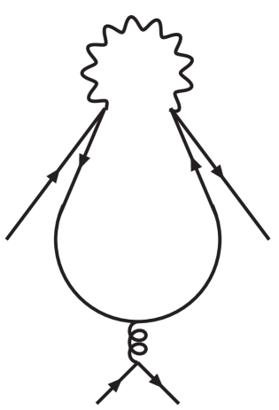
Figure 1: The comparison between a (Linux) Penguin and the Penguin diagram. (Linux Penguin from Neal Tucker, (http://www.isc.tamu.edu/$\sim$lewing/linux/).)

This talk could easily have had other titles, examples are “QCD and Weak Interactions of Light Quarks” or “Penguins and Other Graphs.” In fact I have left out many manifestations of Penguin diagrams. In particular I do not cover the importance in $B$ decays where Penguins were first experimentally verified via $B\to K^{(*)}\gamma$, but are at present more considered a nuisance and often referred to as “Penguin Pollution.” Penguins also play a major role in other Kaon decays, reviews of rare decays where pointers to the literature can be found are Refs [[2, 3, 4]].

In Sect. 2 I give a very short historical overview. Sects 3 and 4 discuss the main physics issues and present the relevant phenomenology of the $\Delta I=1/2$ rule and the $CP$-violating quantities $\varepsilon$ and $\varepsilon^{\prime}/\varepsilon$. The underlying Standard Model diagrams responsible for $CP$-violation are shown there as well. The more challenging part is to actually evaluate these diagrams in the presence of the strong interaction. We can distinguish several regimes of momenta which have to be treated using different methods. An overview is given in Sect. 5 where also the short-distance part is discussed. The more difficult long-distance part has a long history and some approaches are mentioned, but only my favourite method, the $X$-boson or fictitious Higgs exchange, is described in more detail in Sect. 6 where I also present results for the main quantities. For two particular matrix-elements, those of the electroweak Penguins $Q_{7}$ and $Q_{8}$, a dispersive analysis allows to evaluate these in the chiral limit from experimental data. This is discussed in Sect. 7. We summarise our results in the conclusions and compare with the original hopes from Arkady and his collaborators. This talk is to a large extent a shorter version of the review [[5]].

2 A short historical overview

The weak interaction was discovered in 1896 by Becquerel when he discovered spontaneous radioactivity. The next step towards a more fundamental study of the weak interaction was taken in the 1930s when the neutron was discovered and its $\beta$-decay studied in detail. The fact that the proton and electron energies did not add up to the total energy corresponding to the mass of the neutron, made Pauli suggest the neutrino as a solution. Fermi then incorporated it in the first full fledged theory of the weak interaction, the famous Fermi four-fermion [6] interaction.

$${\mathcal{L}}_{\mbox{Fermi}}=\frac{G_{F}}{\sqrt{2}}\;[\overline{p}\gamma_{\mu}\left(1-\gamma_{5}\right)n]\;[\overline{e}\gamma^{\mu}\left(1-\gamma_{5}\right)\nu]\,.$$ (1)

The first fully nonhadronic weak interaction came after world-war two with the muon discovery and the study of its $\beta$-decay. The analogous Lagrangian to Eq. (1) was soon written down. At that point T.D. Lee and C.N. Yang [7] realized that there was no evidence that parity was conserved in the weak interaction. This quickly led to a search for parity violation both in nuclear decays [8] and in the decay chain $\pi^{+}\to\mu^{+}\nu_{\mu}\to e^{+}\nu_{e}\bar{\nu}_{\mu}\nu_{\mu}$.[9] Parity violation was duly observed in both cases. These experiments and others led to the final form of the Fermi Lagrangian given in Eq. (1).[10, 11]

During the 1950s steadily more particles were discovered providing many puzzles. These were solved by the introduction of strangeness,[12, 13] of what is now known as the $K_{L}$ and the $K_{S}$ [14] and the “eightfold way” of classifying the hadrons into symmetry-multiplets.[15]

Subsequently Cabibbo realized that the weak interactions of the strange particles were very similar to those of the nonstrange particles.[16] He proposed that the weak interactions of hadrons occurred through a current which was a mixture of the strange and non-strange currents with a mixing angle now universally known as the Cabibbo angle. The hadron symmetry group led to the introduction of quarks [17] as a means of organising which $SU(3)_{V}$ multiplets were present in the spectrum.

In the same time period the Kaons provided another surprise. Measurements at Brookhaven [18] indicated that the long-lived state, the $K_{L}$, did occasionally decay to two pions in the final state as well, showing that $CP$ was violated. Since the $CP$-violation was small, explanations could be sought at many scales, an early phenomenological analysis can be found in Ref.  [[19]], but as the socalled superweak model [20] showed, the scale of the interaction involved in $CP$-violation could be much higher.

The standard model for the weak and electromagnetic interactions of leptons was introduced in the same period. The Fermi theory is nonrenormalisable. Alternatives based on Yang-Mills [21] theories had been proposed by Glashow [22] but struggled with the problem of having massless gauge bosons. This was solved by the introduction of the Higgs mechanism by Weinberg and Salam. The model could be extended to include the weak interactions of hadrons by adding quarks in doublets, similar to the way the leptons were included. One problem this produced was that loop-diagrams provided a much too high probability for the decay $K_{L}\to\mu^{+}\mu^{-}$ compared to the experimental limits. These socalled flavour changing neutral currents (FCNC) needed to be suppressed. The solution was found in the Glashow-Iliopoulos-Maiani mechanism.[23] A fourth quark, the charm quark, was introduced beyond the up, down and strange quarks. If all the quark masses were equal, the dangerous loop contributions to FCNC processes cancel, the socalled GIM mechanism. This allowed a prediction of the charm quark mass, [24] soon confirmed with the discovery of the $J/\psi$.

In the mean time, QCD was formulated.[25] The property of asymptotic freedom [26] was established which explained why quarks at short distances could behave as free particles and at the same time at large distances be confined inside hadrons.

The study of Kaon decays still went on, and an already old problem, the $\Delta I=1/2$ rule saw the first signs of a solution. It was shown [27, 28] that the short-distance QCD part of the nonleptonic weak decays provided already an enhancement of the $\Delta I=1/2$ weak $\Delta S=1$ transition over the $\Delta I=3/2$ one. The ITEP group extended first the Gaillard-Lee analysis for the charm mass,[29] but then realized that in addition to the effects that were included in Refs [[27, 28]], there was a new class of diagrams that only contributed to the $\Delta I=1/2$ transition.[30, 31] While, as we will discuss in more detail later, the general class of these contributions, the socalled Penguin-diagrams, is the most likely main cause of the $\Delta I=1/2$ rule, the short-distance part of them provide only a small enhancement contrary to the original hope. A description of the early history of Penguin diagrams, including the origin of the name, can be found in the 1999 Sakurai Prize lecture of Vainshtein.[1]

Penguin diagrams at short distances provide nevertheless a large amount of physics. The origin of $CP$-violation was (and partly is) still a mystery. The superweak model explained it, but introduced new physics that had no other predictions. Kobayashi and Maskawa [32] realized that the framework established by Ref. [[23]] could be extended to three generations. The really new aspect this brings in is that $CP$-violation could easily be produced at the weak scale and not at the much higher superweak scale. In this Cabibbo-Kobayashi-Maskawa (CKM) scenario, $CP$-violation comes from the mixed quark-Higgs sector, the Yukawa sector, and is linked with the masses and mixings of the quarks. Other mechanisms at the weak scale also exist, as e.g. an extended Higgs sector.[33]

The inclusion of the CKM mechanism into the calculations for weak decays was done by Gilman and Wise [34, 35] which provided the prediction that $\varepsilon^{\prime}/\varepsilon$ should be nonzero and of the order of $10^{-3}$. Guberina and Peccei [36] confirmed this. This prediction spurred on the experimentalists and after two generations of major experiments, NA48 at CERN and KTeV at Fermilab have now determined this quantity and the qualitative prediction that $CP$-violation at the weak scale exists is now confirmed. Much stricter tests of this picture will happen at other Kaon experiments as well as in $B$ meson studies.

The $K^{0}$-${\overline{K^{0}}}$ mixing has QCD corrections and $CP$-violating contributions as well. The calculations of these required a proper treatment of box diagrams and inclusions of the effects of the $\Delta S=1$ interaction squared. This was accomplished at one-loop by Gilman and Wise a few years later.[37, 38]

That Penguins had more surprises in store was shown some years later when it was realized that the enhancement originally expected on chiral grounds for the Penguin diagrams [30, 31] was present, not for the Penguin diagrams with gluonic intermediate states, but for those with a photon.[39] This contribution was also enhanced in its effects by the $\Delta I=1/2$ rule. This lowered the expectation for $\varepsilon^{\prime}/\varepsilon$, but it became significant after it was found that the top quark had a very large mass. Flynn and Randall [40] reanalysed the electromagnetic Penguin with a large top quark mass and included also $Z^{0}$ exchange. The final effect was that the now rebaptized electroweak Penguins could have a very large contribution that could even cancel the contribution to $\varepsilon^{\prime}/\varepsilon$ from gluonic Penguins. This story still continues at present and the cancellation, though not complete, is one of the major impediments to accurate theoretical predictions of $\varepsilon^{\prime}/\varepsilon$.

The first calculation of two-loop effects in the short-distance part was done in Rome [41] in 1981. The value of $\Lambda_{\mbox{QCD}}$ has risen from values of about 100 MeV to more than 300 MeV. A full calculation of all operators at two loops thus became necessary, taking into account all complexities of higher order QCD. This program was finally accomplished by two independent groups. One in Munich around A. Buras and one in Rome around G. Martinelli.

3 $K\to\pi\pi$ and the $\Delta I=1/2$ rule

The underlying qualitative difference we want to understand is the $\Delta I=1/2$ rule. We can try to calculate $K\to\pi\pi$ decays by simple $W^{+}$ exchange. For $K^{+}\to\pi^{+}\pi^{0}$ we can draw the two Feynman diagrams of Fig. 2(a).

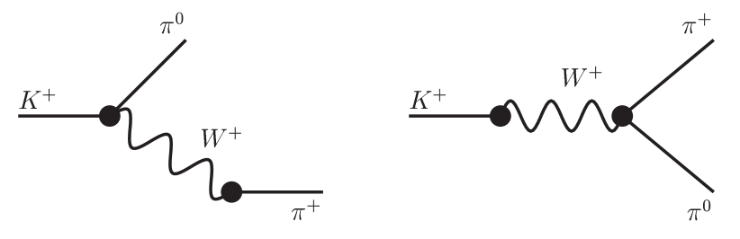
(a)

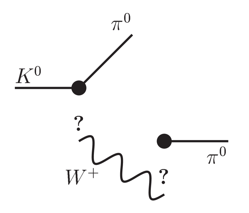
(b)

Figure 2: (a) The two naive $W^{+}$-exchange diagrams for $K^{+}\longrightarrow\pi^{+}\pi^{0}$. (b) No simple $W^{+}$-exchange diagram is possible for $K^{0}\longrightarrow\pi^{0}\pi^{0}$.

The $W^{+}$-hadron couplings are known from semi-leptonic decays. This approximation agrees with the measured decay within a factor of two.

A much worse result appears when we try the same for $K^{0}\to\pi^{0}\pi^{0}$. As shown in Fig. 2(b) there is no possibility to draw diagrams similar to those in Fig. 2(a). The needed vertices always violate charge-conservation. So we expect that the neutral decay should be small compared with the ones with charged pions. Well, if we look at the experimental results, we see

$$\Gamma(K^{0}\longrightarrow\pi^{0}\pi^{0})= \displaystyle\frac{1}{2}\Gamma(K_{S}\longrightarrow\pi^{0}\pi^{0}) =2.3\cdot 10^{-12}\mbox{ MeV}$$

$$\Gamma(K^{+}\longrightarrow\pi^{+}\pi^{0})= \displaystyle 1.1\cdot 10^{-14}\mbox{ MeV}$$ (2)

So the expected zero one is by far the largest !!!

The same conundrum can be expressed in terms of the isospin amplitudes: 

$$A[K^{0}\to\pi^{0}\pi^{0}] \equiv \sqrt{{1}/{3}}{A_{0}}-\sqrt{{2}/{3}}\,{A_{2}}$$

$$A[K^{0}\to\pi^{+}\pi^{-}] \equiv \sqrt{{1}/{3}}{A_{0}}+\sqrt{{1}/{6}}\,{A_{2}}$$

$$A[K^{+}\to\pi^{+}\pi^{0}] \equiv ({\sqrt{3}}/{2}){A_{2}}\,.$$ (3)

The above quoted experimental results can now be rewritten as

$$\left|{A_{0}}/{A_{2}}\right|_{\mbox{exp}}=22$$ (4)

while the naive $W^{+}$-exchange discussed would give

$$\left|{A_{0}}/{A_{2}}\right|_{\mbox{naive}}=\sqrt{2}\,.$$ (5)

This discrepancy is known as the problem of the $\Delta I=1/2$ rule.

Some enhancement comes from final state $\pi\pi$-rescattering. Removing these and higher order effects in the light quark masses one obtains [42, 43]

$$\left|{A_{0}}/{A_{2}}\right|_{\chi}=17.8\,.$$ (6)

This changes the discrepancy somewhat but is still different by an order of magnitude from the naive result (5). The difference will have to be explained by pure strong interaction effects and it is a qualitative change, not just a quantitative one.

We also use amplitudes without the final state interaction phase:

$$A_{I}=-ia_{I}e^{i\delta_{I}}$$ (7)

for $I=0,2$. $\delta_{I}$ is the angular momentum zero, isospin I scattering phase at the Kaon mass.

4 $K\to\pi\pi$, $\varepsilon$, $\varepsilon^{\prime}/\varepsilon$

The $K^{0}$, ${\overline{K^{0}}}$ states have $\bar{s}d$, $\bar{d}s$ quark content. $CP$ acts on these states as

$$CP|K^{0}\rangle=-|{\overline{K^{0}}}\rangle\,.$$ (8)

We can construct eigenstates with a definite $CP$ transformation:

$$K^{0}_{1(2)}=\frac{1}{\sqrt{2}}\left(K^{0}-(+){\overline{K^{0}}}\right),\quad\quad CP|K_{1(2)}=+(-)|K_{1(2)}\,.$$ (9)

The main decay mode of $K^{0}$-like states is $\pi\pi$. A two pion state with charge zero in spin zero is always CP even. Therefore the decay $K_{1}\to\pi\pi$ is possible but $K_{2}\to\pi\pi$ is impossible; $K_{2}\to\pi\pi\pi$ is possible. Phase-space for the $\pi\pi$ decay is much larger than for the three-pion final state. Therefore if we start out with a pure $K^{0}$ or ${\overline{K^{0}}}$ state, the $K_{2}$ component in its wave-function lives much longer than the $K_{1}$ component such that after a long time only the $K_{2}$ component survives.

In the early sixties, as you see it pays off to do precise experiments, one actually measured [18]

$$\frac{\Gamma(K_{L}\to\pi^{+}\pi^{-})}{\Gamma(K_{L}\to\mbox{all})}=(2\pm 0.4)\cdot 10^{-3}\neq 0\,,$$ (10)

showing that $CP$ is violated . This leaves us with the questions:

• Does $K_{1}$ turn in to $K_{2}$ (mixing or indirect $CP$ violation)?

• Does $K_{2}$ decay directly into $\pi\pi$ (direct $CP$ violation)?

In fact, the answer to both is YES  and is major qualitative test of the standard model Higgs-fermion sector and the $CKM$-picture of $CP$-violation.

The presence of $CP$-violation means that $K_{1}$ and $K_{2}$ are not the mass eigenstates, these are

$$K_{S(L)}=\frac{1}{\sqrt{1+|\tilde{\varepsilon}|^{2}}}\left(K_{1(2)}+\tilde{\varepsilon}K_{2(1)}\right)\,.$$ (11)

They are not orthogonal since the Hamiltonian is not hermitian.

We define the observables

$$\varepsilon \equiv \frac{A(K_{L}\to(\pi\pi)_{I=0})}{A(K_{S}\to(\pi\pi)_{I=0})}$$

$$\varepsilon^{\prime} = \frac{1}{\sqrt{2}}\left(\frac{A(K_{L}\to(\pi\pi)_{I=2})}{A(K_{S}\to(\pi\pi)_{I=0})}-\varepsilon\frac{A(K_{S}\to(\pi\pi)_{I=2})}{A(K_{S}\to(\pi\pi)_{I=0})}\right)\,.$$ (12)

The latter has been specifically constructed to remove the $K^{0}$-${\overline{K^{0}}}$ transition. $|\varepsilon|$ is a directly measurable as ratios of decay rates.

We now make a series of experimentally valid approximations,

$$|\mbox{Im}a_{0}|,|\mbox{Im}a_{2}|<<|\mbox{Re}a_{2}|<<|\mbox{Re}a_{0}|,\quad|\varepsilon|,|\tilde{\varepsilon}|<<1,\quad|\varepsilon^{\prime}|<<|\varepsilon|\,,$$ (13)

to obtain the usually quoted expression

$$\varepsilon^{\prime}=\frac{i}{\sqrt{2}}e^{i(\delta_{2}-\delta_{0})}\frac{\mbox{Re}a_{2}}{\mbox{Re}a_{0}}\left(\frac{\mbox{Im}a_{2}}{\mbox{Re}a_{2}}-\frac{\mbox{Im}a_{0}}{\mbox{Re}a_{0}}\right)\,.$$ (14)

Experimentally,[44]

$$|\varepsilon|=(2.271\pm 0.017)\cdot 10^{-3}\,.$$ (15)

The set of diagrams, depicted schematically in Fig. 3(a), responsible for $K^{0}{\overline{K^{0}}}$ mixing are known as box diagrams. It is the presence of the virtual intermediate quark lines of up, charm and top quarks that produces the $CP$-violation.

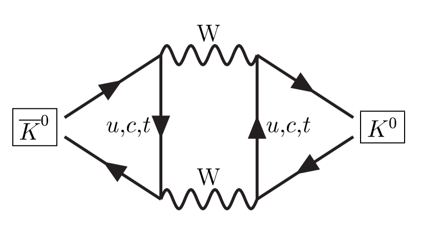
(a)

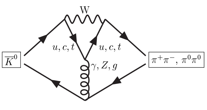
(b)

Figure 3: (a) The box diagram contribution to $K^{0}{\overline{K^{0}}}$ mixing. Crossed versions and diagrams with extra gluons etc. are not shown. (b) The Penguin diagram contribution to $K\to\pi\pi$. Extra gluons and crossed versions etc. are not shown.

The experimental situation on $\varepsilon^{\prime}/\varepsilon$ was unclear for a long time. Two large experiments, NA31 at CERN and E731 at FNAL, obtained conflicting results in the mid 1980’s. Both groups have since gone on and build improved versions of their detectors, NA48 at CERN and KTeV at FNAL. $\varepsilon^{\prime}/\varepsilon$ is measured via the double ratio

$$\mbox{Re}\left(\frac{\varepsilon^{\prime}}{\varepsilon}\right)=\frac{1}{6}\left\{1-\frac{\displaystyle\Gamma(K_{L}\to\pi^{+}\pi^{-})/\Gamma(K_{S}\to\pi^{+}\pi^{-})}{\displaystyle\Gamma(K_{L}\to\pi^{0}\pi^{0})/\Gamma(K_{S}\to\pi^{0}\pi^{0})}\right\}\,.$$ (16)

The two main experiments follow a somewhat different strategy in measuring this double ratio, mainly in the way the relative normalisation of $K_{L}$ and $K_{S}$ components is treated. After some initial disagreement with the first results, KTeV has reanalysed their systematic errors and the situation for $\varepsilon^{\prime}/\varepsilon$ is now quite clear. We show the recent results in Table 4. The data are taken from Ref. [[45]] and the recent reviews in the Lepton-Photon conference.[46, 47]

Recent results on $\varepsilon^{\prime}/\varepsilon$. The years refer to the data sets. NA31 $(23.0\pm 6.5)\times 10^{-4}$ E731 $(7.4\pm 5.9)\times 10^{-4}$ KTeV 96 $(23.2\pm 4.4)\times 10^{-4}$ KTeV 97 $(19.8\pm 2.9)\times 10^{-4}$ NA48 97 $(18.5\pm 7.3)\times 10^{-4}$ NA48 98+99 $(15.0\pm 2.7)\times 10^{-4}$ ALL $(17.2\pm 1.8)\times 10^{-4}$

The Penguin diagram shown in Fig. 3(b) contributes to the direct $CP$-violation as given by $\varepsilon^{\prime}$. Again, $W$-couplings to all three generations show up so $CP$-violation is possible in $K\to\pi\pi$. This is a qualitative prediction of the standard model and borne out by experiment. The main problem is now to embed these diagrams and the simple $W$-exchange in the full strong interaction. The $\Delta I=1/2$ rule shows that there will have to be large corrections to the naive picture.

5 From Quarks to Mesons: a Chain of Effective Field Theories

The full calculation in the presence of the strong interaction is quite difficult. Even at short distances, due to the presence of logarithms of large ratios of scales, a simple one-loop calculation gives very large effects. These need to be resummed which fortunately can be done using renormalisation group methods.

The three steps of the full calculation are depicted in Fig. 4.

ENERGY SCALE	FIELDS	Effective Theory
$M_{W}$	$W,Z,\gamma,g$; $\tau,\mu,e,\nu_{\ell}$; $t,b,c,s,u,d$	Standard Model
	$\Downarrow$ using OPE
$\lesssim m_{c}$	$\gamma,g$; $\mu,e,\nu_{\ell}$; $s,d,u$	QCD,QED, ${\mathcal{H}}_{\mbox{eff}}^{|\Delta S|=1,2}$
	$\Downarrow$ ???
$M_{K}$	$\gamma$; $\mu,e,\nu_{\ell}$; $\pi$, $K$, $\eta$	CHPT

Figure 4: A schematic exposition of the various steps in the calculation of nonleptonic matrix-elements.

First we integrated out the heaviest particles step by step using Operator Product Expansion methods. The steps OPE we describe in the next subsections while step ??? we will split up in more subparts later.

5.1 Step I: from SM to OPE

The first step concerns the standard model diagrams of Fig. 5(a).

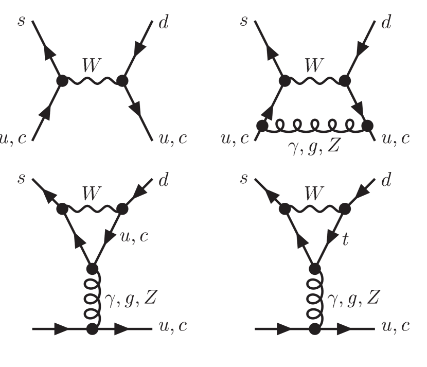
(a)

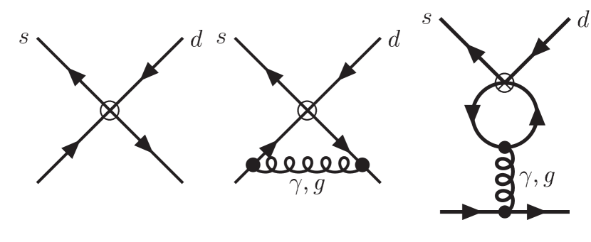
(b)

Figure 5: (a) The standard model diagrams to be calculated at a high scale. (b) The diagrams needed for the matrix-elements calculated at a scale $\mu_{H}\approx m_{W}$ using the effective Hamiltonian.

We replace their effect with a contribution of an effective Hamiltonian given by

$${\mathcal{H}}_{\mbox{eff}}=\sum_{i}C_{i}(\mu)Q_{i}(\mu)=\frac{G_{F}}{\sqrt{2}}V_{ud}V_{us}^{*}\sum_{i}\left(z_{i}-y_{i}\frac{V_{td}V_{ts}^{*}}{V_{ud}V_{us}^{*}}\right)Q_{i}\,.$$ (17)

In the last part we have real coefficients $z_{i}$ and $y_{i}$ and the CKM-matrix-elements occurring are shown explicitly. The four-quark operators $Q_{i}$ can be found in e.g. Ref. [[48]].

We calculate now matrix-elements between quarks and gluons in the standard model using the diagrams of Fig. 5(a) and equate those to the same matrix-elements calculated using the effective Hamiltonian of Eq. (17) and the diagrams of Fig. 5(b). This determines the value of the $z_{i}$ and $y_{i}$. The top quark and the $W$ and $Z$ bosons are integrated out all at the same time. There should be no large logarithms present due to that. The scale $\mu=\mu_{H}$ in the diagrams of Fig. 5(b) of the OPE expansion diagrams should be chosen of the order of the $W$ mass. The scale $\mu_{W}$ in the Standard Model diagrams of Fig. 5(a) should be chosen of the same order.

Notes:
$\bullet$ In the Penguin diagrams $CP$-violation shows up since all 3 generations are present.
$\bullet$ The equivalence is done by calculating matrix-elements between Quarks and Gluons
$\bullet$ The SM part is $\mu_{W}$-independent to $\alpha_{S}^{2}(\mu_{W})$.
$\bullet$ OPE part: The $\mu_{H}$ dependence of $C_{i}(\mu_{H})$ cancels the $\mu_{H}$ dependence of the diagrams to order $\alpha_{S}^{2}(\mu_{H})$.

This procedure gives at $\mu_{W}=\mu_{H}=M_{W}$ in the NDR-scheme  the numerical values given in Table 5.1.

The Wilson coefficients and their main source at the scale $\mu_{H}=m_{W}$ in the NDR-scheme. $z_{1}$ 0.053 $g,\gamma$-box $y_{6}$ $-$0.0019 $g$-Penguin $z_{2}$ 0.981 $W^{+}$-exchange $g,\gamma$-box $y_{7}$ 0.0009 $\gamma,Z$-Penguin $y_{3}$ 0.0014 $g,Z$-Penguin $WW$-box $y_{8}$ 0. $y_{4}$ $-$0.0019 $g$-Penguin $y_{9}$ $-$0.0074 $\gamma,Z$-Penguin $WW$-box $y_{5}$ 0.0006 $g$-Penguin $y_{10}$ 0.

In the same table I have given the main source of these numbers. Pure tree-level $W$-exchange would have only given $z_{2}=1$ and all others zero. Note that the coefficients from $\gamma,Z$ exchange are similar to the gluon exchange ones since $\alpha_{S}$ at this scale is not very big.

5.2 Step II

Now comes the main advantage of the OPE formalism. Using the renormalisation group equations we can calculate the change with $\mu$ of the $C_{i}$, thus resumming the $\log\left(m_{W}^{2}/\mu^{2}\right)$ effects. The renormalisation group equations (RGEs) for the strong coupling and the Wilson coefficients are

$$\mu\frac{d}{d\mu}g_{S}(\mu)=\beta(g_{S}(\mu)),\quad\mu\frac{d}{d\mu}C_{i}(\mu)=\gamma_{ji}(g_{S}(\mu),\alpha)C_{j}(\mu)\,.$$ (18)

$\beta$ is the QCD beta function for the running coupling. The coefficients $\gamma_{ij}$ are the elements of the anomalous dimension matrix $\hat{\gamma}$. They can be derived from the infinite parts of loop diagrams and this has been done to one [50] and two loops.[51] The series in $\alpha$ and $\alpha_{S}$ is known to

$$\hat{\gamma}=\hat{\gamma}^{0}_{S}\frac{\alpha_{S}}{4\pi}+\hat{\gamma}^{1}_{S}\left(\frac{\alpha_{S}}{4\pi}\right)^{2}+\hat{\gamma}_{e}\frac{\alpha}{4\pi}+\hat{\gamma}_{se}\frac{\alpha_{S}}{4\pi}\frac{\alpha}{4\pi}+\cdots$$ (19)

Many subtleties are involved in this calculation.[49, 51] They all are related to the fact that everything at higher loop orders need to be specified correctly, and many things which are equal at tree level are no longer so in $d\neq 4$ and at higher loops, see the lectures [[49]] or the review [[52]]. The numbers below are obtained by numerically integrating Eq. (18).[53, 54]

We perform the following steps to get down to a scale $\mu_{OPE}$ around 1 GeV. Starting from the $z_{i}$ and $y_{i}$ at the scale $\mu_{H}$:
(1) solve Eqs. (18); run from ${\mu_{H}}$ to ${\mu_{b}}$.
(2) At $\mu_{b}$$\approx m_{b}$ remove $b$-quark and match to the theory without $b$ by calculating matrix-elements of the effective Hamiltonian in the five and in the four-quark picture and putting them equal.
(3) Run from $\mu_{b}$ to $\mu_{c}$$\approx m_{c}$.
(4) At $\mu_{c}$ remove the $c$-quark and match to the theory without $c$.
(5) Run from $\mu_{c}$ to $\mu_{\mbox{OPE}}$.
Then all  large logarithms including $m_{W}$, $m_{Z}$, $m_{t}$, $m_{b}$ and $m_{c}$, are summed.

With the inputs $m_{t}(m_{t})=166~{}GeV$, $\alpha=1/137.0$, $\alpha_{S}(m_{Z})=0.1186$ which led to the initial conditions shown in Table 5.1, we can perform the above procedure down to $\mu_{OPE}$. Results for 900 MeV are shown in columns two and three of Table 5.2.

The Wilson coefficients $z_{i}$ and $y_{i}$ at a scale $\mu_{\mbox{OPE}}=$ 900 MeV in the NDR scheme and in the $X$-boson scheme at $\mu_{X}=$ 900 MeV. i         $z_{i}$         $y_{i}$         $z_{i}$         $y_{i}$ $\mu_{OPE}=0.9$ GeV $\mu_{X}=0.9$ GeV $z_{1}$ $-$0.490 0. $-$0.788 0. $z_{2}$ 1.266 0. 1.457 0. $z_{3}$ 0.0092 0.0287 0.0086 0.0399 $z_{4}$ $-$0.0265 $-$0.0532 $-$0.0101 $-$0.0572 $z_{5}$ 0.0065 0.0018 0.0029 0.0112 $z_{6}$ $-$0.0270 $-$0.0995 $-$0.0149 $-$0.1223 $z_{7}$ 2.6$~{}10^{-5}$ $-$0.9$~{}10^{-5}$ 0.0002 $-$0.00016 $z_{8}$ 5.3$~{}10^{-5}$ 0.0013 6.8$~{}10^{-5}$ 0.0018 $z_{9}$ 5.3$~{}10^{-5}$ $-$0.0105 0.0003 $-$0.0121 $z_{10}$ $-$3.6$~{}10^{-5}$ 0.0041 $-$8.7$~{}10^{-5}$ 0.0065

$z_{1}$ and $z_{2}$ have changed much from $0$ and $1$. This is the short-distance contribution to the $\Delta I=1/2$ rule. We also see a large enhancement of $y_{6}$ and $y_{8}$, which will lead to our value of $\varepsilon^{\prime}$.

5.3 Step III: Matrix-elements

Now remember that the $C_{i}$ depend on $\mu_{OPE}$ (scale dependence) and on the definition of the $Q_{i}$ (scheme dependence) and the numerical change in the coefficients due to the various choices for the $Q_{i}$ possible is not negligible. It is therefore important both from the phenomenological and fundamental point of view that this dependence is correctly accounted for in the evaluation of the matrix-elements. We can solve this in various ways.
$\bullet$ Stay in QCD $\Rightarrow$ Lattice calculations.[55]
$\bullet$ ITEP Sum Rules or QCD sum rules. [56]
$\bullet$ Give up $\Rightarrow$ Naive factorisation.
$\bullet$ Improved factorisation
$\bullet$ $X$-boson method (or fictitious Higgs method)
$\bullet$ Large $N_{c}$ (in combination with something like the $X$-boson method.) Here the difference is mainly in the treatment of the low-energy hadronic physics. Three main approaches exist of increasing sophistication.

$\circledast$ CHPT: As originally proposed by Bardeen-Buras-Gérard [57] and now pursued mainly by Hambye and collaborators.[58]

$\circledast$ ENJL (or extended Nambu-Jona-Lasinio model [59]): As mainly done by myself and J. Prades.[60, 48, 61, 53, 54]

$\circledast$ LMD or lowest meson dominance approach.[62] These papers stay with dimensional regularisation throughout. The $X$-boson corrections discussed below, show up here as part of the QCD corrections.

$\bullet$ Dispersive methods Some matrix-elements can in principle be deduced from experimental spectral functions.

Notice that there other approaches as well, e.g. the chiral quark model.[63] These have no underlying arguments why the $\mu$-dependence should cancel, but the importance of several effects was first discussed in this context. I will also not treat the calculations done using bag models and potential models which similarly do not address the $\mu$-dependence issue.

6 The $X$-boson Method and Results using ENJL for the Long Distance

We want to have a consistent calculational scheme that takes the scale and scheme dependence into account correctly. Let us therefore have a closer look at how we calculate the matrix-elements using naive factorisation. We start from the four-quark operator:
$\Rightarrow$ See it as a product of currents or densities.
$\Rightarrow$ Evaluate current matrix-elements in low energy theory or model or from experiment.
$\Rightarrow$ Neglect extra momentum transfer between the current matrix elements.
The main lesson here is that currents and densities are easier to deal with. We also need to go beyond the approximation in the last step. To obtain well defined currents, we replace the four-quark operators by exchanges of fictitious massive $X$-bosons coupling to two-quark currents or densities.

$${\mathcal{H}}=\sum_{i}C_{i}(\mu_{OPE})Q_{i}\quad\Longrightarrow\quad\sum_{i}g_{i}X_{i}J_{i}\,.$$ (20)

$\bullet$ This is a well defined scheme of nonlocal operators.
$\bullet$ The matching to obtain the coupling constants $g_{i}$ from the $C_{i}$ is done with matrix-elements of quarks and gluons.

A simple example is the one needed for the $B_{K}$ parameter. The four-quark operator is replaced by the exchange of one $X$-boson $X_{B}$:

$$C(\mu)\bar{d}\gamma_{\mu}(1-\gamma_{5})s\,\bar{d}\gamma_{\mu}(1-\gamma_{5})s\quad\Longrightarrow\quad g_{B}X_{B}^{\mu}\bar{d}\gamma_{\mu}(1-\gamma_{5})s\,.$$ (21)

Taking a matrix-element between quarks at next-to-leading order in $\alpha_{S}$ gives

$$C(\mu_{OPE})\left(1+r\alpha_{S}(\mu_{OPE})\right)=(g_{B}^{2}/M_{X_{B}}^{2})\left(1+r^{\prime}\alpha_{S}+r^{\prime\prime}\log\left(M_{X_{B}}^{2}/\mu^{2}\right)\right)\,.$$ (22)

The coefficients $r$ and $r^{\prime}$ take care of the scheme dependence. The l.h.s. is scale independent to the required order in $\alpha_{S}$. The effect of these coefficients surprisingly always went in the direction to improve agreement with experiment [48, 54] as can be seen from columns 4 and 5 in Table 5.2.

The final step is the matrix-element of $X_{B}$-boson exchange. For this we split the integral over the $X_{B}$ momentum $q_{X}$ in two parts

$$\int dq_{X}^{2}\Longrightarrow\int_{0}^{\mu^{2}}dq_{X}^{2}+\int_{\mu^{2}}^{\infty}dq_{X}^{2}\,.$$ (23)

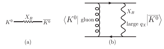
Figure 6: (a) The leading in $1/N_{c}$ contribution from $X_{B}$ exchange. (b) The large momentum part of the $X_{B}$ exchange matrix-element.

The leading in $N_{c}$ contribution is depicted in Fig. 6(a) and corresponds to the large $N_{c}$ factorisation. The large momentum regime is evaluated by the diagram in Fig. 6(b), since the large momentum must flow back through quarks and gluons. Hadronic exchanges are power suppressed because of the form factors involved. The $\alpha_{S}$ present already suppresses by $N_{c}$ so the matrix-element of this part can be evaluated using factorisation. This part cancels the $r^{\prime\prime}\log(M_{X_{B}}^{2}/\mu^{2})$ present in (22). The final part with small $q_{X}$ momentum in the integral then needs to be evaluated nonperturbatively. Here one can use Chiral Perturbation Theory, the ENJL model or meson exchange approximations with various short-distance constraints.

Let me now show some results from Refs [[48, 54]]. The chiral limit coupling $G_{8}$ responsible for the octet contribution, it is 1 in the naive approximation and about 6 when fitted to experiment,[42, 43] is shown in Fig. 7.

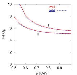
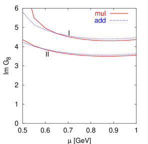
Figure 7: Left: the results for the real part of the octet $\mbox{Re}G_{8}$ as a function of $\mu$. Right: the same for the imaginary part.

As can be seen, the matching between the short and long distance is reasonable both for the real and imaginary parts. The value of $\mbox{Re}G_{8}$ is dominated by the matrix-element of $Q_{1}$ and $Q_{2}$ but about 30-60% comes from the long distance Penguin part of $Q_{2}$. The result for the $\mbox{Im}G_{8}$ corresponds to a value of the $Q_{6}$ matrix-element much larger than usually assumed. We obtained $B_{6}\approx 2$-2.5 while it is usually assumed to be less than 1.5.

Putting our results in (14) we obtain a chiral limit value for $(\varepsilon^{\prime}/\varepsilon)_{\chi}$ of about $6\cdot 10^{-3}$.

We now add the main isospin breaking component $\Omega$ [64] and the effect of final state interaction (FSI).[65] The latter in our case has mainly effect on the forefactor $\mbox{Re}a_{2}/\mbox{Re}a_{0}$ in (14) since the ratios of imaginary parts have been evaluated to the same order in $p^{2}$ in CHPT and thus receive no FSI corrections. The final result is [54] $\varepsilon^{\prime}/\varepsilon\approx 1.5\cdot 10^{-3}$ with an error $\gtrapprox$ 50%.

7 Dispersive Estimates for $\langle Q_{7}\rangle$ and $\langle Q_{8}\rangle$

Some of the matrix-elements we want can be extracted from experimental information in a different way. The canonical example is the mass difference between the charged and the neutral pion in the chiral limit which can be extracted from a dispersive integral over the difference of the vector and axial vector spectral functions.[66]

This idea has been pursued in the context of weak decay in a series of papers by Donoghue, Golowich and collaborators.[67] The matrix-element of $Q_{7}$ could be extracted directly from these data. To get at the matrix-element of $Q_{8}$ is somewhat more difficult. Ref. [[67]] extracted it first by requiring $\mu$-independence, this corresponds to extracting the matrix element of $Q_{8}$ from the spectral functions via the coefficient of the dimension 6 term in the operator product expansion of the underlying Green’s function. The most recent papers using this method are Refs. [[68, 69, 70]] and [[71]]. In the last two papers also some QCD corrections were included which had a substantial impact on the numerical results.

The results are given in Table. 7. The operator $O_{6}^{(1)}$ is related by a chiral transformation to $Q_{7}$ and $O_{6}^{(2)}$ to $Q_{8}$. The numbers are valid in the chiral limit.

The values of the VEVs in the NDR scheme at $\mu_{R}=2$ GeV. The most recent dispersive results are line 3 to 5. The other results are shown for comparison. Errors are those quoted in the papers. Adapted from Ref. [71]. Reference $\langle 0|O_{6}^{(1)}|0\rangle^{NDR}_{\chi}$ $\langle 0|O_{6}^{(2)}|0\rangle^{NDR}_{\chi}$ $B_{7}=B_{8}=1$ $-(5.4\pm 2.2)\cdot 10^{-5}$ GeV⁶ $(1.0\pm 0.4)\cdot 10^{-3}$ GeV⁶ Bijnens et al. [[71]] $-(4.0\pm 0.5)\cdot 10^{-5}$ GeV⁶ $(1.2\pm 0.5)\cdot 10^{-3}$ GeV⁶ Knecht et al. [[68]] $-(1.9\pm 0.6)\cdot 10^{-5}$ GeV⁶ $(2.3\pm 0.7)\cdot 10^{-3}$ GeV⁶ Cirigliano et al. [[70]] $-(2.7\pm 1.7)\cdot 10^{-5}$ GeV⁶ $(2.2\pm 0.7)\cdot 10^{-3}$ GeV⁶ Donoghue et al.[[67]] $-(4.3\pm 0.9)\cdot 10^{-5}$ GeV⁶ $(1.5\pm 0.4)\cdot 10^{-3}$ GeV⁶ Narison [[69]] $-(3.5\pm 1.0)\cdot 10^{-5}$ GeV⁶ $(1.5\pm 0.3)\cdot 10^{-3}$ GeV⁶ lattice [[72]] $-(2.6\pm 0.7)\cdot 10^{-5}$ GeV⁶ $(0.74\pm 0.15)\cdot 10^{-3}$ GeV⁶ ENJL [[54]] $-(4.3\pm 0.5)\cdot 10^{-5}$ GeV⁶ $(1.3\pm 0.2)\cdot 10^{-3}$ GeV⁶

The various results for the matrix-element of $O_{6}^{(1)}$ are in reasonable agreement with each other. The underlying spectral integral, evaluated directly from data in Refs. [[69]],[[70]] and [[71]], or via the minimal hadronic ansatz [[68]] are in better agreement. The largest source of the differences is the way the different results for the underlying evaluation of $O_{6}^{(2)}$ come back into $O_{6}^{(1)}$.

The results for $O_{6}^{(2)}$ are also in reasonable agreement. Ref. [[71]] uses two approaches. First, the matrix-element for $O_{6}^{(2)}$ can be extracted via a similar dispersive integral over the scalar and pseudoscalar spectral functions. The requirements of short-distance matching for this spectral function combined with a saturation with a few states imposes that the nonfactorisable part is suppressed and the number and error quoted follows from this. Extracting the coefficient of the dimension 6 operator in the expansion of the vector and axial-vector spectral functions yields a result comparable but with a larger error of about 0.9. Ref. [[68]] uses a derivation based on a single resonance plus continuum ansatz for the spectral functions and assumes a typical large $N_{c}$ error of 30%. This ansatz worked well for lower moments of the spectral functions which can be tested experimentally. Adding more resonances allows for a broader range of results.[71] Ref. [[70]] chose to enforce all the known constraints on the vector and axial-vector spectral functions to obtain a result. This resulted in rather large cancellations between the various contributions making an error analysis more difficult. A reasonable estimate lead to the value quoted.

The reason why the central value based on the same data can be so different is that the quantity in question is sensitive to the energy regime above 1.3 GeV where the accuracy of the data is rather low.

8 Conclusions

Penguins are alive and well, they provide a sizable part of the $\Delta I=1/2$ enhancement though mainly through long distance Penguin like topologies in the evaluation of the matrix-element of $Q_{2}$. They have found a much richer use in the $CP$ violation phenomenology. For the electroweak Penguins, calculations are in qualitative agreement but more work is still needed to get the errors down. For the strong Penguins, the work I have presented here shows a strong enhancement over factorisation with $B_{6}$ significantly larger than one. The latter conclusion is similar to the one derived from the older more phenomenological arguments where the coefficients were taken at a low scale and the matrix-elements for $Q_{6}$ taken from the the value of the $\Delta I=1/2$ rule. This also indicated a rather large enhancement of the matrix-element of $Q_{6}$ over the naive factorisation.

References

- [1] A. I. Vainshtein, the 1999 Sakurai Prize Lecture, Int. J. Mod. Phys. A14, 4705 (1999) [hep-ph/9906263].
- [2] G. Isidori, hep-ph/9908399, talk KAON99; G. Isidori, hep-ph/0110255; G. Buchalla, hep-ph/0110313.
- [3] L. Littenberg and G. Valencia, Ann. Rev. Nucl. Part. Sci. 43, 729 (1993) [hep-ph/9303225].
- [4] A. J. Buras, “CP violation and rare decays of K and B mesons,” hep-ph/9905437, Lake Louise lectures.
- [5] J. Bijnens, hep-ph/0204068, to be published in ’At the Frontier of Particle Physics/ Handbook of QCD’, edited by M. Shifman, Volume 4.
- [6] E. Fermi, Nuovo Cim. 11, 1 (1934); Z. Phys. 88, 161 (1934).
- [7] T. D. Lee and C. N. Yang, Phys. Rev. 104, 254 (1956).
- [8] C. S. Wu et al., Phys. Rev. 105, 1413 (1957).
- [9] J. I. Friedman and V. L. Telegdi, Phys. Rev. 105, 1681 (1957).
- [10] E. C. Sudarshan and R. E. Marshak, Phys. Rev. 109, 1860 (1958).
- [11] R. P. Feynman and M. Gell-Mann, Phys. Rev. 109, 193 (1958).
- [12] A. Pais,Phys. Rev. 86, 663 (1952).
- [13] M. Gell-Mann, Phys. Rev. 92, 833 (1953).
- [14] M. Gell-Mann and A. Pais,Phys. Rev. 97, 1387 (1955).
- [15] Y. Ne’eman, Nucl. Phys. 26, 222 (1961); M. Gell-Mann, Phys. Rev. 125, 1067 (1962).
- [16] N. Cabibbo, Phys. Rev. Lett. 10, 531 (1963).
- [17] M. Gell-Mann, Phys. Lett. 8, 214 (1964); G. Zweig, CERN report, unpublished.
- [18] J. H. Christenson et al, Phys. Rev. Lett. 13, 138 (1964).
- [19] T. T. Wu and C. N. Yang, Phys. Rev. Lett. 13, 380 (1964).
- [20] L. Wolfenstein, Phys. Rev. Lett. 13, 562 (1964).
- [21] C. N. Yang and R. L. Mills, Phys. Rev. 96, 191 (1954).
- [22] S. L. Glashow, Nucl. Phys. 22, 579 (1961).
- [23] S. L. Glashow, J. Iliopoulos and L. Maiani, Phys. Rev. D2, 1285 (1970).
- [24] M. K. Gaillard and B. W. Lee, Phys. Rev. D10, 897 (1974).
- [25] H. Fritzsch, M. Gell-Mann and H. Leutwyler, Phys. Lett. B47, 365 (1973).
- [26] D. J. Gross and F. Wilczek, Phys. Rev. Lett. 30, 1343 (1973); H. D. Politzer, Phys. Rev. Lett. 30, 1346 (1973).
- [27] M. K. Gaillard and B. W. Lee, Phys. Rev. Lett. 33, 108 (1974).
- [28] G. Altarelli and L. Maiani, Phys. Lett. B52, 351 (1974).
- [29] A. I. Vainshtein, V. I. Zakharov, V. A. Novikov and M. A. Shifman, Sov. J. Nucl. Phys. 23, 540 (1976) [Yad. Fiz. 23, 1024 (1976)].
- [30] A. I. Vainshtein, V. I. Zakharov and M. A. Shifman, JETP Lett. 22, 55 (1975) [Pisma Zh. Eksp. Teor. Fiz. 22, 123 (1975)]; M. A. Shifman, A. I. Vainshtein and V. I. Zakharov, Nucl. Phys. B120, 316 (1977).
- [31] M. A. Shifman, A. I. Vainshtein and V. I. Zakharov, Sov. Phys. JETP 45, 670 (1977) [Zh. Eksp. Teor. Fiz. 72, 1275 (1977)].
- [32] M. Kobayashi and T. Maskawa, Prog. Theor. Phys. 49, 652 (1973).
- [33] S. Weinberg, Phys. Rev. Lett. 37, 657 (1976).
- [34] F. J. Gilman and M. B. Wise, Phys. Lett. B83, 83 (1979).
- [35] F. J. Gilman and M. B. Wise, Phys. Rev. D20, 2392 (1979).
- [36] B. Guberina and R. D. Peccei, Nucl. Phys. B163, 289 (1980).
- [37] F. J. Gilman and M. B. Wise, Phys. Lett. B93, 129 (1980).
- [38] F. J. Gilman and M. B. Wise, Phys. Rev. D27, 1128 (1983).
- [39] J. Bijnens and M. B. Wise, Phys. Lett. B137, 245 (1984).
- [40] J. M. Flynn and L. Randall, Phys. Lett. B224, 221 (1989) [Phys. Lett. B235, 412 (1989)].
- [41] G. Altarelli et al., Phys. Lett. B99, 141 (1981); Nucl. Phys. B187, 461 (1981).
- [42] J. Kambor, J. Missimer and D. Wyler, Phys. Lett. B261, 496 (1991).
- [43] J. Bijnens, P. Dhonte and F. Persson, hep-ph/0205341.
- [44] D. E. Groom et al., Eur. Phys. J. C15, 1 (2000).
- [45] A. Alavi-Harati et al. (KTeV), Phys. Rev. Lett.83, 22 (1999); V. Fanti et al. (NA48), Phys. Lett. B465, 335 (1999); H. Burkhart et al. (NA31), Phys. Lett. B206, 169 (1988); G.D. Barr et al. (NA31), Phys. Lett. B317, 233 (1993); L.K. Gibbons et al. (E731), Phys. Rev. Lett. 70, 1203 (1993)
- [46] R. Kessler, “Recent KTeV results”, hep-ex/0110020 .
- [47] L. Iconomidou-Fayard, NA48 Collaboration, hep-ex/0110028.
- [48] J. Bijnens and J. Prades, J. High Energy Phys. 0001, 002 (2000) [hep-ph/9911392].
- [49] A. J. Buras, hep-ph/9806471, Les Houches lectures.
- [50] Refs. [[27, 28, 30, 34, 35, 36, 39, 40]] and M. Lusignoli, Nucl. Phys. B325, 33 (1989);
-
[51]
A. J. Buras and P. H. Weisz,
Nucl. Phys. B333, 66 (1990);
A. J. Buras et al.,
Nucl. Phys. B370, 69 (1992),
Addendum-ibid. B375, 501 (1992);
A. J. Buras, M. Jamin and M. E. Lautenbacher,
Nucl. Phys. B400, 75 (1993)
[hep-ph/9211321];
A. J. Buras et al.,
Nucl. Phys. B400, 37 (1993)
[hep-ph/9211304];
M. Ciuchini et al., Nucl. Phys. B415, 403 (1994) [hep-ph/9304257]. - [52] G. Buchalla, A. J. Buras and M. E. Lautenbacher, Rev. Mod. Phys. 68, 1125 (1996) [hep-ph/9512380].
- [53] J. Bijnens and J. Prades, J. High Energy Phys. 9901, 023 (1999) [hep-ph/9811472].
- [54] J. Bijnens and J. Prades, J. High Energy Phys. 0006, 035 (2000) [hep-ph/0005189].
- [55] C. T. Sachrajda, hep-ph/0110304; G. Martinelli, hep-ph/0110023.
- [56] M. A. Shifman, A. I. Vainshtein and V. I. Zakharov, Nucl. Phys. B147, 385 (1979); Nucl. Phys. B147, 448 (1979).
- [57] W. A. Bardeen, A. J. Buras and J.-M. Gérard, Phys. Lett. B192, 138 (1987); Nucl. Phys. B293, 787 (1987).
- [58] T. Hambye et al., Phys. Rev. D58, 014017 (1998) [hep-ph/9802300]; T. Hambye, G. O. Köhler and P. H. Soldan, Eur. Phys. J. C10, 271 (1999) [hep-ph/9902334]; T. Hambye et al., Nucl. Phys. B564, 391 (2000) [hep-ph/9906434].
- [59] J. Bijnens, C. Bruno and E. de Rafael, Nucl. Phys. B390, 501 (1993) [hep-ph/9206236]; J. Bijnens, Phys. Rept. 265, 369 (1996) [hep-ph/9502335] and references therein.
- [60] J. Bijnens and J. Prades, Phys. Lett. B342, 331 (1995) [hep-ph/9409255]; Nucl. Phys. B444, 523 (1995) [hep-ph/9502363].
- [61] J. Bijnens, E. Pallante and J. Prades, Nucl. Phys. B521, 305 (1998) [hep-ph/9801326].
- [62] M. Knecht, S. Peris and E. de Rafael, Phys. Lett. B457, 227 (1999) [hep-ph/9812471]; S. Peris and E. de Rafael, Phys. Lett. B490, 213 (2000) [hep-ph/0006146]. E. de Rafael, arXiv:hep-ph/0109280.
- [63] A. Pich and E. de Rafael, Nucl. Phys. B358, 311 (1991); V. Antonelli et al., Nucl. Phys. B469, 143 (1996) [hep-ph/9511255]; V. Antonelli et al., Nucl. Phys. B469, 181 (1996) [hep-ph/9511341]; S. Bertolini, J. O. Eeg and M. Fabbrichesi, Nucl. Phys. B476, 225 (1996) [hep-ph/9512356]; S. Bertolini et al., Nucl. Phys. B514, 93 (1998) [hep-ph/9706260]; S. Bertolini, J. O. Eeg and M. Fabbrichesi, Phys. Rev. D63, 056009 (2001) [hep-ph/0002234]; M. Franz, H. C. Kim and K. Goeke, Nucl. Phys. B562, 213 (1999) [hep-ph/9903275].
- [64] G. Ecker et al., Phys. Lett. B477, 88 (2000) [hep-ph/9912264].
- [65] E. Pallante and A. Pich, Phys. Rev. Lett. 84, 2568 (2000) [hep-ph/9911233]; Nucl. Phys. B592, 294 (2001) [hep-ph/0007208].
- [66] T. Das, G. S. Guralnik, V. S. Mathur, F. E. Low and J. E. Young, Phys. Rev. Lett. 18, 759 (1967).
-
[67]
J. F. Donoghue and E. Golowich,
Phys. Lett. B315, 406 (1993)
[hep-ph/9307263];
Phys. Lett. B478, 172 (2000)
[hep-ph/9911309];
V. Cirigliano and E. Golowich, Phys. Lett. B475, 351 (2000) [hep-ph/9912513];
V. Cirigliano, J. F. Donoghue and E. Golowich, J. High Energy Phys. 0010, 048 (2000) [hep-ph/0007196];
V. Cirigliano and E. Golowich, Phys. Rev. D65, 054014 (2002) [hep-ph/0109265]. - [68] M. Knecht, S. Peris and E. de Rafael, Phys. Lett. B508, 117 (2001) [hep-ph/0102017] and private communication.
- [69] S. Narison, Nucl. Phys. B593, 3 (2001) [hep-ph/0004247]; Nucl. Phys. Proc. Suppl. 96, 364 (2001) [hep-ph/0012019].
- [70] V. Cirigliano, J. F. Donoghue, E. Golowich and K. Maltman, Phys. Lett. B522, 245 (2001) [hep-ph/0109113].
- [71] J. Bijnens, E. Gamiz and J. Prades, J. High Energy Phys. 0110, 009 (2001) [hep-ph/0108240].
- [72] A. Donini et al., Phys. Lett. B470, 233 (1999)