Pion dispersion relation at finite density and temperature

Abstract

We study the behavior of the pion dispersion relation in a pion medium at finite density and temperature. We introduce a pion chemical potential to describe the finite pion number density and argue that such description is valid during the hadronic phase of a relativistic heavy-ion collision between chemical and thermal freeze-out. We make use of an effective Lagrangian that explicitly respects chiral symmetry through the enforcement of the chiral Ward identities. The pion dispersion relation is computed through the computation of the pion self-energy in a non-perturbative fashion by giving an approximate solution to the Schwinger-Dyson equation for this self-energy. The dispersion relation is described in terms of a density and temperature dependent mass and an index of refraction which is also temperature, density as well as momentum dependent. The index of refraction is larger than unity for all values of the momentum for finite $\mu$ and $T$. We conclude by exploring some of the possible consequences for the propagation of pions through the boundary between the medium and vacuum.

I Introduction

The phase structure of hadronic matter at high density and temperature has become a subject of increasing attention in recent years, both from the theoretical and experimental points of view. This attention is driven mainly by the possibility to produce a locally thermalized, deconfined state, whose degrees of freedom are the quarks and gluons of quantum chromodynamics (QCD), the so called quark-gluon plasma (QGP), in high-energy heavy-ion collisions QM01 .

If the QGP is produced in these kind of reactions, the prevailing view portraits the evolution of such a system traversing a series of stages, the last of which consists of a large amount of hadrons strongly interacting in a finite volume, until a final freeze-out.

For not too high temperatures, hadronic matter consists mainly of pions, therefore, the study of the propagation properties of pions within the above described environment represents an important ingredient for the understanding of the properties of the hadronic system at and just before freeze-out. For instance, it has been speculated that the pion interactions within a dense hadronic environment can give rise to interesting collective surface phenomena Shuryak . Moreover, it is also well known that the pion group velocity is an important piece of information necessary to properly account for the dilepton spectrum coming from the hadronic phase Gale-Liu .

The hadronic degrees of freedom are customarily accounted for by means of effective chiral theories that incorporate the Goldstone boson nature of pions. One of such theories is chiral perturbation theory (ChPT) which has been employed to show the well known result that at leading perturbative order and at low momentum, the modification of the pion dispersion curve in a pion medium at finite temperature is just a constant, temperature dependent, increase of the pion mass Gasser . ChPT has also been used in a two-loop computation of the pion self-energy Schenk and decay constant Toublan . A striking result obtained from such computations is that at second order, the shift in the temperature dependence of the pion mass is opposite in sign and about three times larger in magnitude than the first order shift, already at temperatures close to $150$ MeV. This result might signal either the breakdown of the perturbative expansion at these temperatures or the need to perform such calculations using schemes other than perturbation theory.

However, a missing ingredient in the calculations of the pion dispersion curve is the treatment of the medium’s finite density. The conceptual difficulty is related to the fact that, though it is possible to assume that the system is in (at least local) thermal equilibrium, strictly speaking the only conserved charge that can be associated to the pion system is the electric charge and thus, for an electrically neutral pion system the corresponding chemical potential vanishes. The behavior of the pion mass in the presence of an isospin chemical potential has been recently studied in Ref. Loewe . But in order to describe a situation in which the number of pions in thermal equilibrium is finite, we need to consider a chemical potential associated with the pion number, instead of its charge.

Recall that the pion number is not a conserved quantity due to either strong, weak or electromagnetic processes. Nevertheless, the characteristic time for electromagnetic and weak pion number-changing processes, is very large compared to the lifetime of the system created in relativistic heavy-ion collisions and therefore, these processes are of no relevance for the propagation properties of pions within the hadronic phase of the collision. As for the case of strong processes, it is by now accepted that they drive pion number toward chemical freeze-out at a temperature considerably higher than the thermal freeze-out temperature and therefore, that from chemical to thermal freeze-out, the pion system evolves with the pion abundance held fixed Bebie ; Braun-Munzinger . Under these circumstances, it is possible to ascribe to the pion density a chemical potential and consider the pion number as conserved Hung ; Chungsik . In this context, the role of a finite pion chemical potential into a hadronic equation of state has been recently investigated in Ref. Teaney .

Furthermore, another important ingredient in the analysis is the well know fact that in finite temperature field theories with either massless degrees of freedom or that exhibit spontaneous symmetry breaking Dolan , the perturbative expansion breaks down and thus the necessity to implement resummation techniques.

In this paper we explore the effects introduced by a finite pion density on the dispersion curve of pions at finite temperature. Starting from the linear sigma model, we use an effective Lagrangian Ayala obtained by integrating out the heavy sigma modes and compute, in a non perturbative fashion, the pion self-energy. We find that the dispersion curve is modified with respect to the vacuum in a way described by the introduction of an index of refraction larger than one, in addition to the thermal and density increase of the pion mass. We discuss possible implications of such behavior of the pion dispersion curve.

The work is organized as follows: In section II, we recall how for temperatures and momenta smaller than the mass of the sigma, it is possible to integrate out the heavy sigma modes to construct an effective Lagrangian that reproduces the two-loop pion self-energy at finite temperature. In section III, we use this effective Lagrangian to compute non-perturbatively the pion self-energy and from it, the pion dispersion curve at finite density and temperature. Finally, in section IV, we summarize and discuss our results, emphasizing some of the possible consequences of the behavior of the dispersion curve thus found for the propagation pions that approach the boundary between the hadronic medium and vacuum in a relativistic heavy-ion collision.

II Effective Lagrangian

The Lagrangian for the linear sigma model, including only meson degrees of freedom and with an explicit chiral symmetry breaking term, can be written as Lee

$${\mathcal{L}} = \frac{1}{2}\left[(\partial{\mathbf{\pi}})^{2}+(\partial\sigma)^{2}-m_{\pi}^{2}{\mathbf{\pi}}^{2}-m_{\sigma}^{2}\sigma^{2}\right]$$ (1)

$$- \lambda^{2}f_{\pi}\sigma(\sigma^{2}+{\mathbf{\pi}}^{2})-\frac{\lambda^{2}}{4}(\sigma^{2}+{\mathbf{\pi}}^{2})^{2}\,,$$

where $\mathbf{\pi}$ and $\sigma$ are the pion and sigma fields, respectively, and the coupling $\lambda^{2}$ is given by

$$\lambda^{2}=\frac{m_{\sigma}^{2}-m_{\pi}^{2}}{2f_{\pi}^{2}}\,.$$ (2)

From the above Lagrangian one obtains the Green’s functions and Feynman rules to be used in perturbative calculations, in the usual manner. For instance, the bare pion and sigma propagators $\Delta_{\pi}(P)$, $\Delta_{\sigma}(Q)$ and the bare one-sigma two-pion and four-pion vertices $\Gamma_{12}^{ij}$, $\Gamma_{04}^{ijkl}$ are given by (hereafter, capital Roman letters are used to denote four momenta)

$$i\Delta_{\pi}(P)\delta^{ij} = \frac{i}{P^{2}-m_{\pi}^{2}}\delta^{ij}$$

$$i\Delta_{\sigma}(Q) = \frac{i}{Q^{2}-m_{\sigma}^{2}}$$

$$i\Gamma_{12}^{ij} = -2i\lambda^{2}f_{\pi}\delta^{ij}$$

$$i\Gamma_{04}^{ijkl} = -2i\lambda^{2}(\delta^{ij}\delta^{kl}+\delta^{ik}\delta^{jl}+\delta^{il}\delta^{jk})\,.$$ (3)

These Green’s functions are sufficient to obtain the modification to the pion propagator, both at zero and finite temperature, at any given perturbative order.

Figure 1: Diagramatic representation of the self-consistent pion self-energy. The double lines represent the full pion propagator.

When interested in a given approximation scheme to build such Green’s functions, it is possible to exploit the relations that chiral symmetry imposes among them. These relations, better known as chiral Ward identities (ChWI), are a direct consequence of the fact that the divergence of the axial current may be used as an interpolating field for the pion Lee . Thus, one can construct the modification to one of the above Green’s functions at a given perturbative order and for a given approximation. In order to make sure that the approximation respects chiral symmetry, one needs to check that the modification of other Green’s functions respect the corresponding ChWI. For example, two of the ChWI satisfied –order by order in perturbation theory– by the functions $\Delta_{\pi}(P)$, $\Delta_{\sigma}(Q)$, $\Gamma_{12}^{ij}$ and $\Gamma_{04}^{ijkl}$ are

$$f_{\pi}\Gamma_{04}^{ijkl}(;0,P_{1},P_{2},P_{3}) = \Gamma_{12}^{kl}(P_{1};P_{2},P_{3})\delta^{ij}$$

$$+ \Gamma_{12}^{lj}(P_{2};P_{3},P_{1})\delta^{ik}$$

$$+ \Gamma_{12}^{jk}(P_{3};P_{1},P_{2})\delta^{il}$$

$$f_{\pi}\Gamma_{12}^{ij}(Q;0,P) = \left[\Delta_{\sigma}^{-1}(Q)-\Delta_{\pi}^{-1}(P)\right]\delta^{ij}$$ (4)

where momentum conservation at the vertices is implied, that is $P_{1}+P_{2}+P_{3}=0$ and $Q+P=0$. The notation for the functional dependence of the vertices in Eqs. (4) is such that the variables before and after the semicolon refer to the four-momenta of the sigma and pion fields, respectively Lee .

In Refs. Ayala it has been shown that in the kinematical regime where the pion momentum, the pion mass and the temperature are small compared to the sigma mass, the effective one-loop sigma propagator and one-sigma two-pion and four-pion vertices are given by

$$i\Delta_{\sigma}^{\star}(Q) = \frac{i}{Q^{2}-m_{\sigma}^{2}+6\lambda^{4}f_{\pi}^{2}{\mathcal{I}}^{t}(Q)}\,.$$ (5)

$$i\Gamma_{12}^{\star\,ij}(Q;P_{1},P_{2})=-2i\lambda^{2}f_{\pi}\delta^{ij}\left[1-3\lambda^{2}{\mathcal{I}}^{t}(Q)\right]\,,$$ (6)

$$i\Gamma_{04}^{\star\ ijkl}(;P_{1},P_{2},P_{3},P_{4})\!\! = \!\!2i\lambda^{2}\left\{\right.$$

$$\times \!\!\left.\left[1-3\lambda^{2}{\mathcal{I}}^{t}(P_{1}+P_{2})\right]\delta^{ij}\delta^{kl}\right.$$

$$+ \!\!\left[1-3\lambda^{2}{\mathcal{I}}^{t}(P_{1}+P_{3})\right]\delta^{ik}\delta^{jl}$$

$$+ \!\!\left.\left[1-3\lambda^{2}{\mathcal{I}}^{t}(P_{1}+P_{4})\right]\delta^{il}\delta^{jk}\right\},$$

where in the imaginary-time formalism of thermal field theory (TFT), the function ${\mathcal{I}}^{t}$ is obtained as the time-ordered analytical continuation to real energies of the function ${\mathcal{I}}$ defined by

$${\mathcal{I}}(Q) \equiv T\sum_{n}\int\frac{d^{3}k}{(2\pi)^{3}}$$ (8)

$$\times \frac{1}{K^{2}+m_{\pi}^{2}}\,\frac{1}{(K-Q)^{2}+m_{\pi}^{2}}\,.$$

Here $Q=(\omega,{\mathbf{q}}),\,K=(\omega_{n},{\mathbf{k}})$, $Q^{2}=\omega^{2}+q^{2}$, $K^{2}=\omega_{n}^{2}+k^{2}$ with $\omega=2m\pi T$ and $\omega_{n}=2n\pi T$ ($m$, $n$ integers) being discrete boson frequencies, $T$ is the temperature and $q=|{\mathbf{q}}|,\,k=|{\mathbf{k}}|$.

It is easy to check that Eqs. (5), (6) and (LABEL:vert4tot) satisfy the Ward identities in Eq. (4), this ensures that the approximation scheme adopted respects chiral symmetry.

By using the above effective vertices and propagator, it is possible to construct the two-loop modification to the pion self-energy in the same kinematical regime with the result Ayala

$$\Pi_{2}(P) = \left(\frac{m_{\pi}^{2}}{2f_{\pi}^{2}}\right)T\sum_{n}\int\frac{d^{3}k}{(2\pi)^{3}}\frac{1}{K^{2}+m_{\pi}^{2}}$$ (9)

$$\times \left\{3-\left(\frac{m_{\pi}^{2}}{2f_{\pi}^{2}}\right)\left[9{\mathcal{I}}^{t}(0)+6{\mathcal{I}}^{t}(P+K)\right]\right\}.$$

Equation (9) reproduces the leading order result obtained from ChPT Gasser . Furthermore, we observe that Eq. (9) can be formally obtained by means of the effective Lagrangian

$${\mathcal{L}}=\frac{1}{2}\left(\partial_{\mu}{\mathbf{\phi}}\right)^{2}-\frac{1}{2}m_{\pi}^{2}{\mathbf{\phi}}^{2}-\frac{\alpha}{4!}\left({\mathbf{\phi}}^{2}\right)^{2}\,,$$ (10)

where $\alpha=6(m_{\pi}^{2}/2f_{\pi}^{2})$ and the factor $6$ comes from considering the interaction of like-isospin pions in the vertex

$$i\Gamma_{4}^{ijkl}=-2i\left(\frac{m_{\pi}^{2}}{2f_{\pi}^{2}}\right)\left(\delta^{ij}\delta^{kl}+\delta^{ik}\delta^{jl}+\delta^{il}\delta^{jk}\right)\,.$$ (11)

Eqs. (9) and (10) mean that in the kinematical regime where the sigma mass is large compared to the pion mass, the momentum and the temperature, the linear sigma model Lagrangian reduces to a $\phi^{4}$ Lagrangian for effective like-isospin pions with an effective coupling given by $\alpha$. By restricting ourselves to the above kinematical regime, we will proceed on working with the Lagrangian given by Eq. (10).

III Non-perturbative pion self-energy

It is well know that quantum field theories at finite temperature present certain subtleties such as the breakdown of the perturbative expansion Kapusta . This breakdown becomes manifest in two important cases: the appearance of infrared divergences in theories with massless degrees of freedom, and the compensation of powers of the coupling constant with powers of $T$ for large temperatures. In both situations, the resummation of certain classes of diagrams represents an important improvement for the study of the physical properties of such theories. Even for cases where neither there is a massless degree of freedom, nor the temperature is extremely large, it is important to consider a resummation scheme, particularly for the case of theories with spontaneous symmetry breaking near critical behavior.

In order to consider the above mentioned general situation and with the purpose of studying the pion dispersion curve at finite density and temperature, let us formally consider the Schwinger-Dyson equation for the pion self-energy depicted in Fig. 1, whose analytic expression is given by

$$\Pi(P) = \frac{\alpha}{2}T\sum_{n}\int\frac{d^{3}k}{(2\pi)^{3}}\frac{1}{K^{2}+m_{\pi}^{2}+\Pi}$$

$$- \frac{\alpha^{2}}{6}T^{2}\sum_{n_{1},n_{2}}\int\frac{d^{3}k_{1}}{(2\pi)^{3}}\frac{d^{3}k_{2}}{(2\pi)^{3}}\frac{1}{K_{1}^{2}+m_{\pi}^{2}+\Pi}$$

$$\times \frac{1}{K_{2}^{2}+m_{\pi}^{2}+\Pi}\frac{1}{(K_{1}+K_{2}-P)^{2}+m_{\pi}^{2}+\Pi}\,,$$

where for internal lines, we make the substitution $i\omega\rightarrow i\omega+\mu$. Notice that since the interaction Lagrangian contains only a quartic term, there is no need to dress the vertices in the above equation.

Equation (LABEL:SD) represents an integral equation for the function $\Pi(P)$, which, needless to say, is very difficult to be solved exactly. In order to find an approximate solution let us write

$$\Pi(P)\simeq\Pi_{0}+\tilde{\Pi}(P)$$ (13)

and consider $\tilde{\Pi}(P)\ll\Pi_{0}$. As we will see, such assumption is justified given that in our approximation, $\tilde{\Pi}\sim{\mathcal{O}}(\alpha^{2})$. Keeping only the lowest order contribution in $\tilde{\Pi}$, Eq. (LABEL:SD) becomes

$$\Pi(P) \equiv \Pi_{0}+\tilde{\Pi}(P)$$

$$= \frac{\alpha}{2}T\sum_{n}\int\frac{d^{3}k}{(2\pi)^{3}}\frac{1}{K^{2}+m_{\pi}^{2}+\Pi_{0}}$$

$$- \frac{\alpha^{2}}{6}T^{2}\sum_{n_{1},n_{2}}\int\frac{d^{3}k_{1}}{(2\pi)^{3}}\frac{d^{3}k_{2}}{(2\pi)^{3}}\frac{1}{K_{1}^{2}+m_{\pi}^{2}+\Pi_{0}}$$

$$\times \frac{1}{K_{2}^{2}+m_{\pi}^{2}+\Pi_{0}}\frac{1}{(K_{1}+K_{2}-P)^{2}+m_{\pi}^{2}+\Pi_{0}}\,,$$

which in turn, serves as the definition of the functions $\Pi_{0}$ and $\tilde{\Pi}(P)$, given by

$$\Pi_{0}\equiv\frac{\alpha}{2}T\sum_{n}\int\frac{d^{3}k}{(2\pi)^{3}}\frac{1}{K^{2}+m_{\pi}^{2}+\Pi_{0}}\,,$$ (15)

$$\tilde{\Pi}(P) \equiv -\frac{\alpha^{2}}{6}T^{2}\sum_{n_{1},n_{2}}\int\frac{d^{3}k_{1}}{(2\pi)^{3}}\frac{d^{3}k_{2}}{(2\pi)^{3}}\frac{1}{K_{1}^{2}+m_{\pi}^{2}+\Pi_{0}}$$

$$\times \frac{1}{K_{2}^{2}+m_{\pi}^{2}+\Pi_{0}}\frac{1}{(K_{1}+K_{2}-P)^{2}+m_{\pi}^{2}+\Pi_{0}}\,.$$

Equation (15) represents a self consistent equation for the (momentum independent) constant $\Pi_{0}$. This is the well known resummation for the superdaisy diagrams which constitute the dominant contribution in the large-$N$ expansion Dolan of the Lagrangian in Eq. (10). On the other hand, Eq. (LABEL:pitilde) represents a first approximation to the momentum dependent piece of $\Pi(P)$.

The solution to Eq. (15) is given by the transcendental equation

$$\Pi_{0} = \left(\frac{\alpha T}{4\pi}\right)\sqrt{m_{\pi}^{2}+\Pi_{0}}$$ (17)

$$\times \sum_{n=1}^{\infty}K_{1}\left(\frac{n\sqrt{m_{\pi}^{2}+\Pi_{0}}}{T}\right)\frac{\cosh(n\mu/T)}{n}\,.$$

Figure 2 shows the behavior of the quantity $\sqrt{m_{\pi}^{2}+\Pi_{0}}$ as a function of $(a)$ the temperature $T$ for different values of the chemical potential $\mu$ and $(b)$ as a function of $\mu$ for different values of $T$. In both cases, $\sqrt{m_{\pi}^{2}+\Pi_{0}}$ grows monotonically with both $T$ and $\mu$.

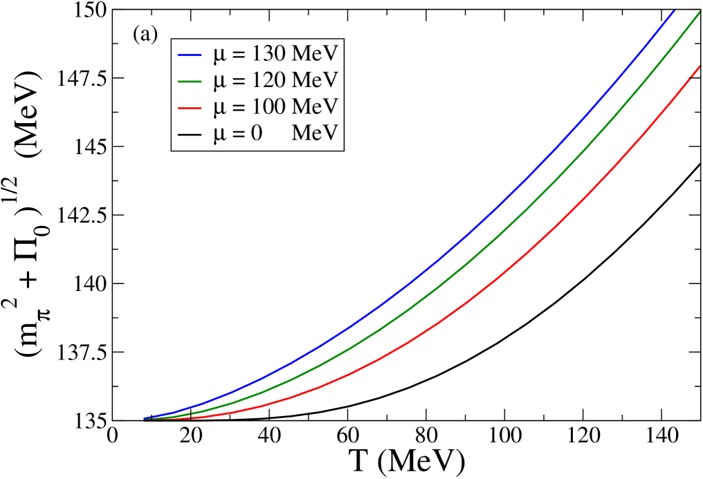
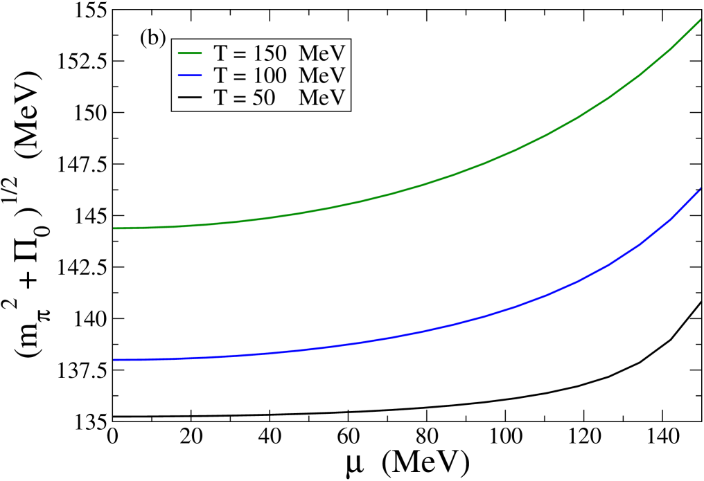
Figure 2: $\sqrt{m_{\pi}^{2}+\Pi_{0}}$ as a function of $(a)$ the temperature $T$ for different values of the chemical potential ranging from $\mu=0$ to $\mu=130$ MeV and as a function of $(b)$ the chemical potential $\mu$ for different values of the temperature ranging from $T=50$ to $T=150$ MeV.

The calculation of the function $\tilde{\Pi}(P)$ involves that of the function

$${\mathcal{S}}(P)\equiv T\sum_{n}\int\frac{d^{3}k}{(2\pi)^{3}}\frac{{\mathcal{I}}(K;\sqrt{m_{\pi}^{2}+\Pi_{0}})}{(K-P)^{2}+m_{\pi}^{2}+\Pi_{0}}\,,$$ (18)

where ${\mathcal{I}}(K;\sqrt{m_{\pi}^{2}+\Pi_{0}})$ is the function defined in Eq. (8), with the replacement $m_{\pi}\rightarrow\sqrt{m_{\pi}^{2}+\Pi_{0}}$. The calculation of the dispersion relation requires knowledge of the real part of the retarded version of the function ${\mathcal{S}}(P)$, which, after analytical continuation to real frequencies, is given by LeBellac

$${\mbox{R}}{\mbox{e}}{\mathcal{S}}^{r}(p_{0},p)\!\!\! \equiv \!\!\!\frac{1}{2}\left[{\mathcal{S}}(i\omega\rightarrow p_{0}+i\epsilon,p)\right.$$

$$+ \!\!\!\left.{\mathcal{S}}(i\omega\rightarrow p_{0}-i\epsilon,p)\right]$$

$$= \!\!\!\ -\ {\mathcal{P}}\int\frac{d^{3}k}{(2\pi)^{3}}\int_{-\infty}^{\infty}\frac{dk_{0}}{2\pi}\int_{-\infty}^{\infty}\frac{dk_{0}^{\prime}}{2\pi}$$

$$\!\!\!\left[1+f(k_{0}+\mu)+f(k_{0}^{\prime}-\mu)\right]2\ {\mbox{I}}{\mbox{m}}{\mathcal{I}}^{t}(k_{0},k)$$

$$\!\!\!\frac{2\pi\ \varepsilon(k_{0}^{\prime})\ \delta[{k_{0}^{\prime}}^{2}-({\mathbf{k}}-{\mathbf{p}})^{2}-m_{\pi}^{2}-\Pi_{0}]}{p_{0}-k_{0}-k_{0}^{\prime}},$$

where ${\mathcal{P}}$ stands for the principal part of the integral, $\varepsilon$ is the sign function and

$$f(x)=\frac{1}{e^{x/T}-1}$$ (20)

is the Bose-Einstein distribution.

From Eq. (LABEL:reS) we see that we require only knowledge of the imaginary part of ${\mathcal{I}}^{t}(k_{0},k)$. It is a lengthy, though straightforward exercise to show that

$${\mbox{I}}{\mbox{m}}{\mathcal{I}}^{t}(k_{0},k)\!\!\! = \!\!\!-\frac{1}{16\pi}\Theta[K^{2}-4(m_{\pi}^{2}+\Pi_{0})]$$ (21)

$$\times \!\!\!\{[a(K^{2})+\frac{2T}{k}\ln\left(\frac{1-e^{-[\omega_{+}(k_{0},k)+\mu]/T}}{1-e^{-[\omega_{-}(k_{0},k)+\mu]/T}}\right)]$$

$$\times \!\!\!\Theta(k_{0})$$

$$+ \!\!\![a(K^{2})+\frac{2T}{k}\ln\left(\frac{1-e^{-[\omega_{+}(k_{0},k)-\mu]/T}}{1-e^{-[\omega_{-}(k_{0},k)-\mu]/T}}\right)]$$

$$\times \!\!\!\Theta(-k_{0})\}\,,$$

where $K^{2}=k_{0}^{2}-k^{2}$, $\Theta$ is the step function and the functions $a$ and $\omega_{\pm}$ are

$$a(K^{2}) = \sqrt{1-\frac{4(m_{\pi}^{2}+\Pi_{0})}{K^{2}}}$$

$$\omega_{\pm}(k_{0},k) = \frac{|k_{0}|\pm a(K^{2})k}{2}\,.$$ (22)

It can also be checked that for $\mu=0$, Eqs. (21) and (22) reduce to the corresponding expressions found in Refs. Ayala .

Figure 3: $p_{0}$ as a function of $p$ for $\mu=0,120,130$ MeV and $T=120$ MeV.

Notice that Eq. (LABEL:reS) contains temperature-dependent infinities coming from the terms involving the function ${\mathcal{I}}^{t}$, as well as vacuum infinities. This is an usual feature of multi-loop calculations at finite temperature where one always encounters temperature-dependent infinities in integrals involving only the bare terms of the original Lagrangian. However, as it turns out, these infinities are exactly canceled by the contribution from the integrals computed by using the counterterms that are necessary to introduce at the previous order of the loop expansion to carry the (vacuum) renormalization. This renormalization method has been developed in Refs. Caldas for the resummation method employed here and has been given the name Modified Self-Consistent Resummation. For the purposes of this work, we concentrate on the finite, temperature-dependent terms and refer the reader to the above cited works for a detailed treatment of the renormalization procedure.

According to Eqs. (LABEL:pitilde) and (18)

$${\mbox{R}}{\mbox{e}}\tilde{\Pi}^{r}(p_{0},p)=-\frac{\alpha^{2}}{6}{\mbox{R}}{\mbox{e}}{\mathcal{S}}^{r}(p_{0},p)\,,$$ (23)

therefore, the pion dispersion relation is given as the solution to

$$p_{0}^{2}-\left[p^{2}+m_{\pi}^{2}+\Pi_{0}-\frac{\alpha^{2}}{6}{\mbox{R}}{\mbox{e}}{\mathcal{S}}^{r}(p_{0},p)\right]=0$$ (24)

for positive $p_{0}$. Figure 3 shows plots of $p_{0}$ as a function of $p$ for different values of $\mu$ and a temperature $T=120$ MeV. As can be seen from this figure, $\Pi(p_{0},p=0)$ contributes to the increase of the pion mass. Also, for large $p$, the dispersion curves approach the light cone, always from within the causal region $p_{0}^{2}>p^{2}$.

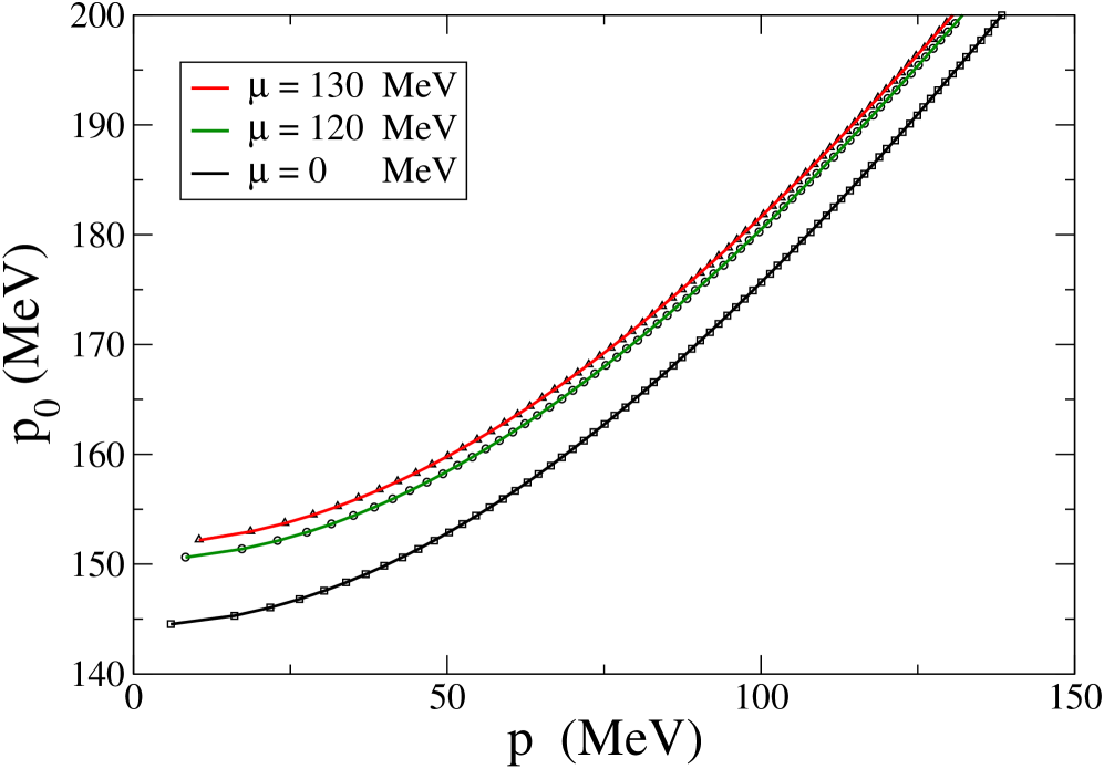
Figure 4: Fit of the dispersion curve to the functional form $p_{0}=\sqrt{n^{-1}(T,\mu)p^{2}+M^{2}(T,\mu)}$ for $\mu=0,120,130$ MeV and $T=120$ MeV. The dots are the computed values of the dispersion relation.

We also notice that the dispersion curves can be parametrized by a function of the form

$$p_{0}=\sqrt{n^{-1}(T,\mu)p^{2}+M^{2}(T,\mu)}\,.$$ (25)

This is shown in Fig. 4 where the dots represent the computed values of the dispersion relation and the continuous curves the fits. Table 1 shows the values of the parameters $n(T,\mu)$ and $M(T,\mu)$ for the different values of $\mu$ and the temperature considered. From this table we observe that the presence of a finite chemical potential has two dramatic effects on the behavior of the pion dispersion curve compared to the case where only the temperature is considered: first, there is a significant increase in the pion mass and second, the index of refraction parameter $n$ becomes larger than unity.

Recall that the magnitude of the pion group velocity $v_{g}$ is given as the derivative of the pion energy $p_{0}$ with respect to the momentum $p$. From Eq. (25) we see that

$$v_{g} \equiv \frac{dp_{0}}{dp}$$ (26)

$$= n^{-1}\left(\frac{p}{p_{0}}\right)$$

$$= n^{-1}\left(\frac{p}{p_{0}^{\mbox{\tiny vac}}}\right)\left(\frac{p_{0}^{\mbox{\tiny vac}}}{p_{0}}\right)$$

$$= v_{g}^{\mbox{\tiny vac}}/\tilde{n}(p)\,,$$

where we have defined the (momentum dependent) index of refraction $\tilde{n}(p)$ as

$$\tilde{n}(p)=n\left(\frac{p_{0}}{p_{0}^{\mbox{\tiny vac}}}\right)\,,$$ (27)

and the vacuum pion group velocity $v_{g}^{\mbox{\tiny vac}}$ as

$$v_{g}^{\mbox{\tiny vac}}=\left(\frac{p}{p_{0}^{\mbox{\tiny vac}}}\right)\,.$$ (28)

Equation (27) can be interpreted as a temperature, density, and momentum-dependent pion index of refraction. Since for finite $T$ and $\mu$, we always have both $n>1$ and $p_{0}/p_{0}^{\mbox{\tiny vac}}>1$, for all values of $p$, the index of refraction developed by the pion medium at finite density and temperature is always larger than unity.

$\mu$ (MeV)	$n$	$M$ (MeV)
0	1	144.411
120	1.004	150.388
130	1.006	151.826

Table 1: Values of the parameters $n(T,\mu)$ and $M(T,\mu)$, for three values of the chemical potential, $\mu=0,120,130$ MeV and for a temperature $T=120$ MeV.

IV Summary and conclusions

In this paper we have considered the effects of a finite pion density on the pion dispersion curve at finite temperature. The finite density is described in terms of a finite pion chemical potential. We have argued that such description is valid during the hadronic phase of a collision of heavy nuclei at high energies between chemical and thermal freeze-out when the strong pion-number changing processes have driven the pion number to a fixed value.

In order to consider a general scenario that takes into account resummation effects, we have presented an approximate solution to the Schwinger-Dyson equation for the momentum-dependent pion self-energy, writing this as $\Pi(P)\simeq\Pi_{0}+\tilde{\Pi}(P)$ and considering $\tilde{\Pi}(P)\ll\Pi_{0}$, which is justified given that in our approximation, $\tilde{\Pi}\sim{\mathcal{O}}(\alpha^{2})$, whereas the perturbative expansion of $\Pi_{0}$ starts at ${\mathcal{O}}(\alpha)$.

The pion dispersion relation thus obtained at finite density and temperature deviates from the vacuum dispersion relation and can be described in terms of a density and temperature dependent mass and an index of refraction, also temperature, density as well as momentum dependent. This index of refraction is larger than unity for all values of the momentum. Similar results have been obtained in Ref. Pisarski using also a linear sigma model without the introduction of a finite chemical potential but rather as a consequence of the loss of Lorentz invariance when a particle travels in a medium at finite temperature. We note however that our result is more general than that of the former reference where the computation of the pion dispersion relation was carried from the onset in the weak coupling regime, that is to say, $\lambda^{2}\ll 1$, whereas our approach is valid for arbitrary values of $\lambda^{2}$ Ayala .

A very interesting consequence of the development of such index of refraction happens when considering pions that approach the boundary between the strongly interacting hadronic region of the collision and vacuum. Propagation through the boundary wall can be described in three different regimes, depending on whether the wall’s width $d$ is much smaller, on the order of, or much larger than the pion’s wave length $\lambda$. In the first situation (thin wall regime), it is possible to treat the propagation of the pions through the boundary in terms of transmission and reflection coefficients. In the second case, diffusion effects have to be properly taken into account. However, in the third case ($d\ll\lambda$), which we choose here as an illustrative scenario, it is possible to consider the motion of pions through the wall as that of classical particles climbing out of a potential well and the interaction of the wall on the pions as that of a classical force that causes the momentum component normal to the boundary, $p_{t}$, to change, while the momentum component parallel to the boundary, $p_{l}$, is left unchanged Shuryak . The change is found by imposing energy conservation for the waves on both sides of he wall

$$\sqrt{n^{-1}(T,\mu)p_{\mbox{\tiny in}}^{2}+M^{2}(T,\mu)}=\sqrt{p_{\mbox{\tiny out}}^{2}+m_{\pi}^{2}}$$ (29)

which in turn implies

$$(p_{t}^{2})_{\mbox{\tiny out}}=n^{-1}(p_{t}^{2})_{\mbox{\tiny in}}-p_{l}^{2}[1-n^{-1}]+[M^{2}-m_{\pi}^{2}]\,.$$ (30)

Notice that when $n=1$, Eq. (30) means that the momentum component normal to the boundary in vacuum grows when compared to the same component inside the pion medium. However, in the general case of finite $T$ and $\mu$, $n^{-1}<1$ so, from Eq. (30) we see that it is possible that for certain values of $p_{l}$, $p_{l}^{2}[1-n^{-1}]\geq n^{-1}(p_{t}^{2})_{\mbox{\tiny in}}+[M^{2}-m_{\pi}^{2}]$ and thus that $(p_{t})_{\mbox{\tiny out}}$ be zero or purely imaginary, meaning that the pion is reflected back.

These phenomena might have a word on the behavior of the transverse pion spectra measured from SIS (Heavy Ion Synchrotron) to RHIC energies, but clearly a more detailed study of the propagation properties of pions through the boundary between the hadronic phase and vacuum in relativistic heavy-ion collisions is called for. This will be the subject of a future work progress .

References

- (1) For a recent review see Quark Matter ’01, Proceedings of the 15th International Conference on Ultra-Relativistic Nucleus-Nucleus Collisions, Nucl. Phys. A698, 1 (2002).
- (2) E. V. Shuryak, Phys. Rev. D 42, 1764 (1990).
- (3) C. Gale and J. Kapusta, Phys. Rev. C 35, 2107 (1987); L. C. Liu and W.-H. Ma, ibid 43, R935 (1991).
- (4) J. Gasser and H. Leutwyler, Phys. Lett. B 184, 83 (1987).
- (5) A. Schenk, Phys. Rev. D 47, 5138 (1993).
- (6) D. Toublan, Phys. Rev. D 56, 5629 (1997).
- (7) M. Loewe and C. Villavicencio, Thermal pions at finite density, hep-ph/0206294, (2002).
- (8) H. Bebie, P. Gerber, J.L. Goity and H. Leutwyler, Nucl. Phys. B 378, 95 (1992).
- (9) P. Braun-Munzinger, J. Stachel, J. Wessels, and N. Xu, Phys. Lett. B 344, 43 (1995), ibid 365, 1 (1996).
- (10) C.M. Hung and E. Shuryak, Phys. Rev. C 57, 1891 (1998).
- (11) C. Song and V. Koch, Phys. Rev. C 55, 3026 (1997).
- (12) D. Teaney, Chemical freezeout in heavy ion collisions, nucl-th/0204023 (2002).
- (13) L. Dolan and R. Jackiw, Phys. Rev. D 9, 3320 (1974); S. Weinberg, ibid 9, 3357 (1974).
- (14) A. Ayala, S. Sahu and M. Napsuciale, Phys. Lett. B 479, 156 (2000); A. Ayala and S. Sahu, Phys. Rev. D 62, 056007 (2000).
- (15) B. W. Lee, Chiral Dynamics (Gordon and Breach, New York, 1972).
- (16) J.I. Kapusta, Finite Temperature Field Theory (Cambridge University Press, Cambridge, 1989).
- (17) M. Le Bellac, Thermal Field Theory (Cambridge University Press, Cambridge, 1996).
- (18) H.C.G. Caldas, A.L. Mota and M.C. Nemes, Phys. Rev. D 63, 056011 (2001); H.C.G. Caldas, ibid 65, 065005 (2002).
- (19) R.D. Pisarski and M. Tytgat, Phys. Rev. D 64, R2989 (1996).
- (20) A. Ayala, work in progress.