MPI-PhT 2002-25

hep-ph/0206201

June 2002

Reshuffling the OPE:
Delocalized Operator Expansion

A. H. Hoang and R. Hofmann

Max-Planck-Institut für Physik
Werner-Heisenberg-Institut
Föhringer Ring 6, 80805 München
Germany

A prescription for the short-distance expansion of Euclidean current correlators based on a delocalized modification of the multipole expansion of perturbative short-distance coefficient functions is proposed that appreciates the presence of nonlocal physics in the nonperturbative QCD vacuum. This expansion converges better than the local Wilson OPE, which is recovered in the limit of infinite resolution. As a consequence, the usual local condensates in the Wilson OPE become condensates that depend on a resolution parameter and that can be expressed as an infinite series of local condensates with increasing dimension. In a calculation of the nonperturbative correction to the ground state energy level of heavy quarkonia the improved convergence properties of the delocalized expansion are demonstrated. Phenomenological evidence is gathered that the gluon condensate, often being the leading nonperturbative parameter of the Wilson OPE, is indeed a function of resolution. The delocalized expansion is applied to derive a leading order scaling relation for $f_{D}/f_{B}$ in the heavy mass expansion.

1 Introduction

Establishing a connection between universal parameters of the nonperturbative QCD vacuum in Euclidean space-time on the one hand and an integral over weighted hadronic cross sections on the other hand has proven to be a very fruitful idea. [1] The three underlying assumptions of this approach are the analyticity of correlators of gauge invariant currents, the existence of a meaningful (asymptotic) large-momentum expansion of these correlators in the Euclidean region and the possibility of a dual description for hadron dynamics in terms of the dynamics of quarks and gluons. One may wonder whether these assumptions really are all independent. Given our poor analytic understanding of the nonperturbative quantum dynamics of quarks and gluons at present, we are not in a position to prove the analyticity assumption in QCD from first principles. On the other hand, one may, on general grounds and with the help of results from lattice gauge theory, try to connect the issue of a meaningful large-momentum expansion with that of quark-hadron duality.

The conventional approach to the large-momentum expansion of the correlator of a gauge invariant QCD current $j(x)$ is Wilson’s operator product expansion (OPE),

$$i\int d^{4}x\,\mbox{e}^{iqx}\left\langle\,Tj(x)j^{\dagger}(0)\,\right\rangle\,=\,Q^{2}\sum_{N=0}\sum_{l=1}^{l_{N}}\,c_{Nl}(Q^{2})\,\left\langle O_{Nl}(0)\right\rangle\ ,\ \ (Q^{2}=-q^{2}>0)\ .$$ (1)

In Eq. (1) the contribution with $N=0$ is solely due to perturbation theory, whereas $N>0$ runs over the dimension of the local and gauge invariant composite operators $O_{Nl}(0)$, and $l$ labels operators of the same dimension. Operators $O_{N_{1}l_{1}}(0)$ and $O_{N_{2}l_{2}}(0)$ with $N_{1}<N_{2}$ need not be unrelated. Rather, $O_{N_{2}l_{2}}(0)$ may be the result of gauge-covariant differentiations of the gauge invariant $k$-point function corresponding to the content of fundamental fields in the local operator $O_{N_{1}l_{1}}(0)$. [1] In this sense $O_{N_{2}l_{2}}(0)$ is a reducible operator. It is the purpose of this paper to exploit the relation of a chain of reducible local operators with nonlocal vacuum averages for constructing a modified version of the OPE.

According to the standard interpretation [1], the physics of low-momentum, nonperturbative vacuum fluctuations resides in the vacuum averages $\left\langle O_{Nl}(0)\right\rangle$, whereas high-momentum, perturbative propagation is contained in the Wilson coefficients $c_{Nl}(Q^{2})$. If $\left\langle O_{Nl}(0)\right\rangle\sim\Lambda^{N}$ then, apart from logarithmic factors arising from anomalous, perturbative operator scaling, we have $c_{Nl}(Q^{2})\sim Q^{-N}$. Here it is assumed that $Q$ is the only relevant short-distance scale. Nonperturbative corrections to the $N=0$ contribution are counted in powers of $\Lambda/Q$ and are small if $\Lambda\ll Q$, and if $l_{N}$ is sufficiently small. It is expected that the OPE is asymptotic at best, i.e.  convergence is only apparent up to some critical value of $N$.

The expansion into vacuum averages of local operators assumes correlations in the vacuum to be rigid, or in other words, it is assumed that the lower bound on the correlation lengths of the corresponding nonlocal gauge invariant $k$-point functions is considerably larger than the short-distance scale $Q^{-1}$. More specifically, one likes to think of correlation lengths being of the order $\Lambda^{-1}\sim\Lambda_{\rm QCD}^{-1}$, where $\Lambda_{\rm QCD}$ is the typical hadronization scale, i.e. it is commonly assumed that there is no hierarchy in nonperturbative scales.

Given the exact knowledge of all gauge invariant QCD vacuum correlators and maintaining the possibility to factorize perturbative propagation from nonperturbative background fluctuations for each operator structure, one may view the OPE (1) as a degenerate multipole expansion of the perturbative part. To see this, we consider the simplified case of a nonperturbative and nonlocal dimension-4 structure corresponding to a slowly varying 2-point correlator $g(x)$ falling off at distance $\Delta_{g}\sim\Lambda^{-1}$ in its Euclidean space-time argument $x$. It is straightforward to generalize the subsequent considerations to arbitrary $n$-point correlators. In addition, we consider a short-distance function $f(x)$, calculable in perturbation theory, that probes the vacuum at distance $x\sim\Delta_{f}\sim Q^{-1}$. Since the function $f(x)$ describes short-distance physics at the scale $Q\gg\Lambda$ it is strongly peaked compared to $g(x)$ (see Fig. 1). For demonstration purposes it suffices to consider an effectively one-dimensional problem in which the chain of local power corrections to the purely perturbative result reads

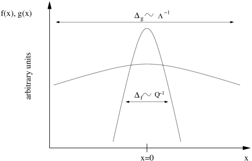
Figure 1: Schematic drawing of the short-distance function $f(x)$ and the 2-point-correlator $g(x)$ illustrating the scale hierarchy $\Delta_{f}/\Delta_{g}\sim\Lambda/Q\ll 1$.

$$\int_{-\infty}^{\infty}dx\,f(x)\,g(x) = \int dx\,dy\,f(y)\,\delta(x-y)\,g(x)$$ (2)

$$= \int dx\,dy\,f(y)\,\bigg{[}\,\sum_{n=0}^{\infty}\frac{(-1)^{n}}{n!}\,y^{n}\delta^{(n)}(x)\,\bigg{]}\,g(x)$$

$$= \sum_{n=0}^{\infty}\bigg{[}\,\int dy\,f(y)\,y^{n}\,\bigg{]}\,\left[\int dx\,\frac{(-1)^{n}}{n!}\delta^{(n)}(x)\,g(x)\right]$$

$$= \sum_{n=0}^{\infty}\,\bigg{[}\left.\,\bigg{(}i\frac{d}{dk}\bigg{)}^{n}\,\tilde{f}(k)\right|_{k=0}\,\bigg{]}\,\bigg{[}\,\int\frac{dk}{2\pi}\,\frac{(ik)^{n}}{n!}\,\tilde{g}(k)\,\bigg{]}\,.\quad$$

The functions $\tilde{f}$ and $\tilde{g}$ are the Fourier transforms of $f$ and $g$, respectively. From Eq. (2) it follows that

$$f(x) = \sum_{n=0}^{\infty}\,\bigg{[}\,\int dy\,f(y)\,y^{n}\,\bigg{]}\,\frac{(-1)^{n}}{n!}\,\delta^{(n)}(x)\,,$$ (3)

which is an expansion into degenerated multipoles. In electrodynamics the 3-dimensional generalization of Eq. (3) is used to determine the potential of a localized and static charge distribution $\rho(x)$ at distances much larger than its spatial extension (see e.g. Ref. [2]). The first term on the RHS of Eq. (3) corresponds to the total charge times the delta function located at the center of the charge distribution, the second term corresponds to the dipole moment times the derivative of the delta function, etc.. In the chain of local power corrections the derivatives of $\delta$-functions generate higher-dimensional operators that are obtained by covariant differentiations of the correlator $g(x)$ at the origin $x=0$. We note that without specifying a regularization scheme the terms in the series of Eq. (2) do only exist, if the functions $f$ and $g$ fall off sufficiently fast in the infrared and the ultraviolet, respectively. For $g$ this statement translates to the property that the local operators, which are contained in the corresponding chain, do not have anomalous dimensions. The presence of anomalous dimensions implies a regularization scheme, which we will ignore in this introduction and in Secs. 2–5.

Briefly switching to 4 dimensions, we now give an example for gauge invariant two-point correlations leading to the function $g(x)$. The field strength correlator [3]

$$g_{\mu\nu\kappa\lambda}(x)\,\equiv\,\mbox{Tr}\,\left\langle g^{2}\,G_{\mu\nu}(x)\,S(x,0)\,G_{\kappa\lambda}(0)\,S(0,x)\,\right\rangle\,,$$ (4)

where

$$S(x,y)\,=\,{\cal P}\,\mbox{e}^{ig\int_{0}^{x}dz_{\mu}A_{\mu}(z)}\,,$$ (5)

generates the following chain of vacuum expectation values (VEV’s) involving local operators of increasing dimension

$$\mbox{Tr}\,\left\langle g^{2}\,G_{\mu\nu}(0)\,G_{\kappa\lambda}(0)\right\rangle,\$$ (7)

$$\mbox{Tr}\,\left\langle g^{2}\,G_{\mu\nu}(0)\,D_{\rho}\,G_{\kappa\lambda}(0)\right\rangle,\ \mbox{Tr}\,\left\langle g^{2}\,G_{\mu\nu}(0)\,D_{\tau}D_{\rho}\,G_{\kappa\lambda}(0)\right\rangle,\ \ldots\ ,$$

This can most easily be seen in Schwinger’s fixed point gauge $x_{\mu}A_{\mu}(x)=0$ [4] if one assumes that the integration path in Eq. (5) is a straight line. In the limit, where $R\equiv\Delta g/\Delta f\to\infty$, the lowest power correction dominates, and operators such as in Eq. (7) are irrelevant in the OPE. The correlator of Eq. (4) depends on the closed path containing the points $0$ and $x$. For the purpose of lattice evaluations a straight line is always assumed. This may be adequate for the extraction of the highest mass nonperturbative scale being present in the corresponding gauge invariant correlations.

The first VEV in Eq. (7) is called the gluon condensate and VEV’s with odd numbers of covariant derivatives do not contribute due to the experimentally well justified parity and time-reversal invariance of the QCD Lagrangian. Perturbatively, one can define the gluon condensate in such a way that its anomalous dimension vanishes to all orders in $\alpha_{s}$. [5] For the channels, which we will consider later, the anomalous dimension of the dimension six condensates are small. [1] We will therefore ignore the problem of anomalous dimensions in these applications. We will come back to this issue in Sec. 6.

Let us carry on assuming a one-dimensional world. Retaining only the lowest power correction at $R<\infty$ corresponds to a saddle point approximation of the $x$-integral in (2). Expressed somewhat loosely in mathematical terms, the strongly peaked function $f$ and the slowly varying function $g$ lie in a dual space defined with respect to the bilinear form

$$(f,g)\,\equiv\,\int dx\,f(x)\,g(x)\,.$$ (8)

Formally, the set of functions

$$e_{n}(x)\,\equiv\,\frac{(-1)^{n}}{n!}\,\delta^{(n)}(x)\qquad\mbox{and}\qquad\tilde{e}_{n}(x)\,\equiv\,x^{n}\,,$$ (9)

which are used to construct the multipole expansion in Eq. (3), span a basis of the dual space, with the orthonormality relation

$$\left(\,e_{n}\,,\,\tilde{e}_{m}\,\right)\,=\,\delta_{nm}\,.$$ (10)

The series of corrections to the saddle-point approximation, which involve the covariant derivatives of $g(x)$ at $x=0$, is in general only asymptotic, and it is intuitively clear that the convergence properties worsen for $R$ approaching unity. Much better convergence properties may be achieved by utilizing a multipole expansion of $f(x)$ which starts out with a saddle point approximation based on an function of width $\Delta_{f}\approx Q^{-1}$ instead of the infinitely narrow $\delta$-function. In this paper we present an explicit construction of such an expansion and apply it to determine a modified version of the local OPE in Eq. (1). We refer to this expansion as “delocalized operator expansion” (DOE).

The observation that the local expansion from Eq. (1) breaks down for $R$ approaching unity and that the corrections to the saddle-point approximation can be substantial is well known and has led in the past to a number of phenomenological studies considering directly the non-local form in the first line of Eq. (2) without any expansion. [6, 7, 8, 9] In these studies the importance of including non-local effects has been demonstrated in a number of cases. In this approach the short-distance function $f(x)$ has to be computed for arbitrary values of $x$ and a specific ansatz for the form of the non-perturbative correlator $g(x)$ has to be adopted. This leads to the unpleasant features that the determination of the perturbative short-distance function is considerably more complicated than for the Wilson coefficients of the local expansion, particularly a higher loop level, and that it necessarily involves some model-dependence which makes the estimates of theoretical errors difficult. The DOE has been constructed with the aim to provide an alternative formalism for non-local effects. The DOE can be applied with a definite power counting like the local OPE and keeps the computational advantages of the local expansion in the determination of the short-distance coefficients. The new feature of the DOE is that it relies on a generalization of the multipole expansion of the short-distance function $f(x)$ based on functions having a width that can be adjusted to the short-distance scale $Q$. This leads to an improved convergence of the expansion for the price of having to introduce an additional parameter $\Omega$ which we call “resolution scale”. The condensates in the DOE depend on $\Omega$ and this dependence accounts for non-local effects. The DOE can be used to extract model-independent information on the non-local structure of the non-perturbative QCD vacuum with a well defined power counting (Sec. 5), but also to simplify the determination of numerical predictions in a given model for the form of non-perturbative correlation functions $g(x)$ (Secs. 4 and 6).

The outline of the paper is as follows. In Sec. 2 we introduce the framework of the DOE assuming that the factorization of long- and short-distance fluctuations can be carried out without ambiguities. The delocalized expansion is associated with a resolution parameter $\Omega$ and, for $\Omega\sim Q$, can lead to a series that has better convergence properties than the local OPE. Matrix elements in the DOE systematically sum an infinite series of local operators at each order in $\Lambda/Q$. At lowest order in $\Lambda/Q$ the DOE implies an $\Omega$-dependent running gluon condensate. In Sec. 3 we review what is known about the gauge invariant gluonic field strength correlator from lattice simulations. In Sec. 4 the nonperturbative corrections to the ground state energy of a heavy quarkonium system are calculated in the local and the delocalized expansion in $\Lambda/mv^{2}$. Using a lattice-inspired model for the gluon field strength correlator, we show that the DOE has better asymptotic convergence than the local OPE. Section 5 contains an extraction of the gluon condensate from experimental data using charmonium sum rules and the Adler function in the $V+A$ channel of light quark pair production. We find evidence that the gluon condensate is indeed running. We show that our results are consistent with the lattice measurements of the gluonic field strength correlator. In Sec. 6 we show how the DOE is constructed for the more general case that the factorization of long- and short-distance fluctuations is ambiguous and needs to be carried out in a regularization scheme. We then apply the DOE to derive a scaling relation for the ratio of meson decay constants $f_{D}/f_{B}$ at leading order in the heavy mass expansion. A summary and an outlook are given in Sec. 7. Finally, in App. A we show that the gluon field strength correlator has approximately the same tensor structure as the local gluon condensate, which simplifies computations in the investigations in the main body of the paper. Appendix B contains analytical formulae for the local short-distance coefficients needed for the examination of quarkonium energy levels in Sec. 4.

2 Delocalized operator expansion: framework,
evolutions equations and power counting

To construct a modified version of the multipole expansion used in Eq. (3) we need to find a generalization of the basis functions in Eq. (9) satisfying an orthonormality relation in analogy to Eq. (10). In Ref. [10] a lowest-order analysis based on a 4-dimensional spherical well was performed. Here, we construct a basis of the dual space by appealing to the orthonormality properties of the Hermite polynomials and their duals. For a treatment in Cartesian coordinates the following basis is well suited:

$$e_{n}^{\Omega}(x) \equiv \frac{\Omega^{n+1}}{\sqrt{\pi}\,n!}\,H_{n}(\Omega x)\,\mbox{e}^{-\Omega^{2}x^{2}}\,,$$

$$\tilde{e}_{n}^{\Omega}(x) \equiv \frac{H_{n}(\Omega x)}{(2\,\Omega)^{n}}\,.$$ (11)

For even values of $n$ the first three Hermite polynomials read

$$H_{0}(x)\,=\,1\,,\qquad H_{2}(x)\,=\,4x^{2}-2\,,\qquad H_{4}(x)\,=\,16x^{4}-48x^{2}+12\,.$$ (12)

The width of the basis functions $e_{n}^{\Omega}$ is of order $\Omega^{-1}$, and one recovers the basis of the local expansion in the limit $\Omega\to\infty$:

$$e_{n}^{\Omega}\,\stackrel{{\scriptstyle\Omega\to\infty}}{{\longrightarrow}}\,e_{n}\qquad\mbox{and}\qquad\tilde{e}_{n}^{\Omega}\,\stackrel{{\scriptstyle\Omega\to\infty}}{{\longrightarrow}}\,\tilde{e}_{n}\,.$$ (13)

An expansion of $f(x)g(x)$ using the resolution dependent basis $\{e_{n}^{\Omega},\tilde{e}_{n}^{\Omega}\}$ generates the following representation of the $x$-integral in Eq. (2)

$$\int_{-\infty}^{\infty}dx\,f(x)\,g(x) = \sum_{n=0}^{\infty}f_{n}(\Omega)\,g_{n}(\Omega)\,,$$ (14)

where

$$f_{n}(\Omega)\,\equiv\,(\,f\,,\,\tilde{e}^{\Omega}_{n}\,) = \int dx\,f(x)\,\frac{H_{n}(\Omega x)}{(2\,\Omega)^{n}}$$ (15)

$$= \left.\frac{1}{(2\,\Omega)^{n}}\,H_{n}\bigg{(}\Omega\bigg{(}i\frac{d}{dk}\bigg{)}\bigg{)}\,\tilde{f}(k)\right|_{k=0}\,,$$

$$g_{n}(\Omega)\,\equiv\,(\,e^{\Omega}_{n}\,,\,g\,) = \int dx\,\frac{\Omega^{n+1}}{\sqrt{\pi}\,n!}\,H_{n}(\Omega x)\,\mbox{e}^{-\Omega^{2}x^{2}}\,g(x)$$ (16)

$$= \int\frac{dk}{2\pi}\,\frac{(ik)^{n}}{n!}\,\mbox{e}^{-\frac{k^{2}}{4\Omega^{2}}}\,\tilde{g}(k)\,.$$

We call $\Omega$ the “resolution parameter”. It is intuitively clear that the series in Eq. (14) has better convergence properties, if $\Omega$ is of order $Q$, because in this case the term $(f,\tilde{e}_{0}^{\Omega})e_{0}^{\Omega}(x)$ accounts much better for the form of $f(x)$ than for $\Omega=\infty$. The terms $f_{n}(\Omega)$ are the resolution-dependent short-distance coefficients, and the $g_{n}(\Omega)$ are the resolution-dependent condensates. Note that, if $f(x)$ is positive definite within its main support $|x|\,<\,Q^{-1}$, then $f_{n}(\infty)>0$ for $n$ not too large. On the other hand, if $g(x)$ is positive definite and monotonic decreasing for $x>0$, then $g_{n}(\Omega)<g_{n}(\Omega^{\prime})$ for $\Omega<\Omega^{\prime}$.

The relation between basis functions for different resolution parameters $\Omega$ and $\Omega^{\prime}$ can be obtained from the properties of the Hermite polynomials and reads

$$\tilde{e}_{n}^{\Omega}(x) = \sum_{m=0}^{\infty}a_{nm}(\Omega,\Omega^{\prime})\,\tilde{e}_{m}^{\Omega^{\prime}}(x)$$

$$e_{n}^{\Omega}(x) = \sum_{m=0}^{\infty}a_{mn}(\Omega^{\prime},\Omega)\,e_{m}^{\Omega^{\prime}}(x)\,,$$ (17)

where

$$a_{nm}(\Omega,\Omega^{\prime})\,=\,\left\{\begin{array}[]{ll}\frac{\displaystyle n!}{{\displaystyle m!}\,\big{(}\mbox{$\frac{n-m}{2}$}\big{)}!}\,\bigg{(}{\displaystyle\frac{\Omega^{2}-\Omega^{\prime\,2}}{4\,\Omega^{2}\,\Omega^{\prime\,2}}}\bigg{)}^{\big{(}\mbox{$\frac{n-m}{2}$}\big{)}}\,,&n-m\geq 0\,\,\mbox{and even}\,,\\[17.07164pt] 0\,,&\mbox{otherwise}\,.\end{array}\right.$$ (18)

Equation (18) leads to the following relations between the short-distance coefficients $f_{n}$ and the corresponding condensates $g_{n}$ for different resolutions $\Omega$ and $\Omega^{\prime}$:

$$f_{n}(\Omega) = \sum_{m=0}^{\infty}a_{nm}(\Omega,\Omega^{\prime})\,f_{m}(\Omega^{\prime})$$ (19)

$$g_{n}(\Omega) = \sum_{m=0}^{\infty}a_{mn}(\Omega^{\prime},\Omega)\,g_{m}(\Omega^{\prime})\,.$$ (20)

The coefficients $a_{nm}(\Omega,\Omega^{\prime})$ satisfy the composition property

$$\sum_{i=0}^{\infty}a_{ni}(\Omega,\Omega^{\prime})\,a_{im}(\Omega^{\prime},\Omega^{\prime\prime})\,=\,a_{nm}(\Omega,\Omega^{\prime\prime})\,,$$ (21)

and for equal resolution we have

$$a_{nm}(\Omega,\Omega)\,=\,\delta_{nm}\,.$$ (22)

Obviously, the transformations $a_{nm}(\Omega,\Omega^{\prime})$ form a group. It is instructive to specify the relations in Eqs. (19) and (20) for $\Omega^{\prime}=\infty$,

$$f_{0}(\Omega) = f_{0}(\infty)\,,$$

$$f_{2}(\Omega) = f_{2}(\infty)\,-\,\frac{1}{2\,\Omega^{2}}f_{0}(\infty)\,,$$

$$f_{4}(\Omega) = f_{4}(\infty)\,-\,\frac{3}{\Omega^{2}}f_{2}(\infty)\,+\,\frac{3}{4\,\Omega^{4}}\,f_{0}(\infty)\,,$$

$$\vdots$$

$$f_{n}(\Omega) = \sum_{i=0}^{[n/2]}\frac{n!}{(n-2i)!\,i!}\left(-\frac{1}{4\Omega^{2}}\right)^{i}\,f_{n-2i}(\infty)\,,$$

$$g_{n}(\Omega) = \sum_{i=n}^{\infty}\,\frac{(n+2i)!}{n!\,i!}\,\Big{(}\frac{1}{4\,\Omega^{2}}\Big{)}^{i}\,g_{n+2i}(\infty)\,,$$ (23)

where the explicit expressions for $f_{n}(\infty)$ and $g_{n}(\infty)$ can be read off Eq. (2). We see that each short-distance coefficient $f_{n}(\Omega)$ can be expressed in terms of a finite linear combination of the local Wilson coefficients $f_{i}(\infty)$ for $i\leq n$. In particular, the short-distance coefficient $f_{0}(\Omega)$ and the Wilson coefficient of the first term in the local expansion coincide since $H_{0}(\Omega x)=1$, i.e. the short-distance coefficient in the saddle-point approximation is $\Omega$-independent. On the other hand, the resolution-dependent condensates $g_{n}(\Omega)$ are related to an infinite sum of local condensates with additional covariant derivatives multiplied by $\Omega$-dependent coefficients. From now on we adopt the language saying that resolution-dependent condensates of a given dimension can be expressed as an infinite sum of local condensates of equal and higher dimension. And similarly we say that each resolution-dependent short-distance coefficient associated with a condensate of a certain dimension can be expressed as a finite sum of local short-distance coefficients associated with condensates of equal or smaller dimensions.

Note that in Eq. (14) the term $f_{0}(\infty)g_{2}(\infty)/(2\Omega^{2})$ contained in $f_{0}(\Omega)g_{0}(\Omega)$ is cancelled by the term $-f_{0}(\infty)g_{2}(\infty)/(2\Omega^{2})$ in $f_{2}(\Omega)g_{2}(\Omega)$ which exemplarily shows the reshuffling of the OPE. As we have argued above, the Wilson coefficients $f_{n}(\infty)$ have equal sign for $n$ not too large and therefore the short-distance coefficient $f_{2}(\Omega)$ can be much smaller than $f_{2}(\infty)$ for $\Omega\sim Q$. This feature and the fact that $g_{n}(\Omega)<g_{n}(\infty)$ under the conditions mentioned above can, at least for small $n$, severely suppress higher order contributions. The DOE of the current correlator in Eq. (1) has the same parametric counting in powers of $\Lambda/Q$ as the OPE, as long as $\Omega$ is not chosen parametrically smaller than $Q$. Taking into account that $g_{n}\sim\Lambda^{n}$ and $f_{n}\sim Q^{-n}$ in the local expansion, we also have

$$g_{n}(\Omega)\sim\Lambda^{n}\sum_{i}\Big{(}\frac{\Lambda}{\Omega}\Big{)}^{i}\sim\Lambda^{n}\,,\qquad f_{n}(\Omega)\sim Q^{-n}\sum_{i}\Big{(}\frac{Q}{\Omega}\Big{)}^{i}\sim Q^{-n}\quad\mbox{}$$ (24)

in the DOE as long as $\Omega\gg Q$. At finite resolution, however, one obtains additional summations of powers of $Q/\Omega$ and $\Lambda/\Omega$ in the short-distance coefficients and the condensates, respectively. Adopting a lattice-inspired model, we will see in Sec. 4 that for $\Omega\sim Q$ the expansion in powers of $\Lambda/Q$ has an additional suppression by powers of a small number as compared to the expansion for $\Omega=\infty$.

It is straightforward to extend the previous results to an arbitrary number of dimensions by applying the resolution-dependent expansion independently to each coordinate. This also accounts for the treatment of arbitrary $n$-point correlations in an arbitrary number of dimensions. For convenience we consider here the same resolution parameter $\Omega$ for each coordinate. It is straightforward to derive the resolution-dependent expansion for a more general situation.

If $f=f(x_{1},\ldots,x_{d})$ is a strongly peaked short-distance function in $d$ dimensional Euclidean space-time the analogous expansion to Eq. (14) reads

$$\int_{-\infty}^{\infty}d^{d}x\,f(x_{1},\ldots,x_{d})\,g(x_{1},\ldots,x_{d}) = \sum_{n_{1},\ldots,n_{d}=0}^{\infty}f_{n_{1},\ldots,n_{d}}(\Omega)\,g_{n_{1},\ldots,n_{d}}(\Omega)\,,\quad$$ (25)

where

$$f_{n_{1},\ldots,n_{d}}(\Omega) \equiv \int d^{d}x\,f(x_{1},\ldots,x_{d})\,\bigg{[}\,\prod_{i=1}^{d}\frac{H_{n_{i}}(\Omega x_{i})}{(2\,\Omega)^{n_{i}}}\,\bigg{]}$$ (26)

$$= \left.\bigg{[}\,\prod_{i=1}^{d}\,\frac{1}{(2\,\Omega)^{n_{i}}}\,H_{n_{i}}\bigg{(}\Omega\bigg{(}i\frac{d}{dk_{i}}\bigg{)}\bigg{)}\,\bigg{]}\,\tilde{f}(k_{i},\ldots,k_{d})\right|_{k_{1},\ldots,k_{d}=0}\,,$$

$$g_{n_{1},\ldots,n_{d}}(\Omega) \equiv \int d^{d}x\,\bigg{[}\,\prod_{i=1}^{d}\frac{\Omega^{n_{i}+1}}{\sqrt{\pi}\,n_{i}!}\,H_{n_{i}}(\Omega x_{i})\,\bigg{]}\,\mbox{e}^{-\Omega^{2}x^{2}}\,g(x_{1},\ldots,x_{d})$$ (27)

$$= \int\frac{d^{d}k}{(2\pi)^{d}}\,\bigg{[}\,\prod_{i=1}^{d}\,\frac{(ik_{n_{i}})^{n_{i}}}{n_{i}!}\,\bigg{]}\,\mbox{e}^{-\frac{k^{2}}{4\Omega^{2}}}\,\tilde{g}(k_{1},\ldots,k_{d})\,.$$

The relation between the short-distance coefficients and the condensates in Eqs. (26) and (27) for different resolution parameters is derived from Eqs. (17) for each index $n_{i}$ in analogy to the expressions in Eqs. (19) and (20). As in the one-dimensional case each short-distance coefficient $f_{n_{1},\ldots,n_{d}}(\Omega)$ can be expressed in terms of a finite linear combination of the local Wilson coefficients $f_{i_{1}\ldots,i_{d}}(\infty)$ for $i_{k}\leq n_{k}$, and the short-distance coefficient $f_{0,\ldots,0}(\Omega)$ is resolution-independent. The resolution-dependent condensates $g_{n_{1},\ldots,n_{d}}(\Omega)$ are related to an infinite sum of local condensates $g_{i_{1},\ldots,i_{d}}(\infty)$ for $i_{k}\geq n_{k}$. For example, assuming that $g$ is a function of the distance $|x|=(x_{1}^{2}+\ldots+x_{d}^{2})^{1/2}$ only, one finds

$$g_{0,\ldots,0}(\Omega) = g_{0,\ldots,0}(\infty)+\frac{1}{2Q^{2}}\,\Big{(}\,g_{2,\ldots,0}(\infty)+\ldots+g_{0,\ldots,2}(\infty)\,\Big{)}+\ldots$$ (28)

$$= g(0)+\frac{1}{4Q^{2}}\partial_{\rho}\partial_{\rho}g(0)+\ldots\,.$$

It is an easy exercise to derive evolution equations for the resolution-dependent short-distance coefficients and the condensates. In the one-dimensional case the evolution equations are obtained directly from Eqs. (19) and (20) and read

$$\frac{d}{d\,\Omega}\,f_{n}(\Omega) = \frac{(n-1)\,n}{2\,\Omega^{3}}\,f_{n-2}(\Omega)\,,$$

$$\frac{d}{d\,\Omega}\,g_{n}(\Omega) = -\,\frac{(n+1)(n+2)}{2\,\Omega^{3}}\,g_{n+2}(\Omega)\,.$$ (29)

Equations (29) imply that there is only mixing between terms that differ by two mass dimensions. This is a consequence of the specific choice of the basis functions in Eqs. (11), which are constructed from the Hermite polynomials and the Gaussian function. For the short-distance coefficients lower dimensional terms always mix into higher dimensional ones. Prescribing short-distance coefficients at $\Omega=\infty$, the solutions are given by Eqs. (23). For the condensates higher dimensional terms always mix into lower dimensional ones. Their evolution equations are much more interesting because they show that knowing the leading condensate $g_{0}(\Omega)$ implies that all subleading condensates of higher dimensions are obtained by differentiations with respect to $\Omega$. The analogous features also exist for the $d$-dimensional generalization of the evolution equations, which have the form

$$\frac{d}{d\,\Omega}\,f_{n_{1},\ldots,n_{d}}(\Omega) = \frac{(n_{1}-1)\,n_{1}}{2\,\Omega^{3}}\,f_{n_{1}-2,\ldots,n_{d}}(\Omega)+\ldots+\frac{(n_{d}-1)\,n_{d}}{2\,\Omega^{3}}\,f_{n_{1},\ldots,n_{d}-2}(\Omega)\,,$$

$$\frac{d}{d\,\Omega}\,g_{n_{1},\ldots,n_{d}}(\Omega) = -\,\frac{(n_{1}+1)(n_{1}+2)}{2\,\Omega^{3}}\,g_{n_{1}+2,\ldots,n_{d}}(\Omega)-$$ (30)

$$\hskip 28.45274pt\ldots-\frac{(n_{d}+1)(n_{d}+2)}{2\,\Omega^{3}}\,g_{n_{1},\ldots,n_{d}+2}(\Omega)\,.$$

3 The gluonic field strength correlator

Since it is the most important 2-point function, which hence we will heavily draw upon in subsequent sections, we review here what is known from lattice calculations about the gauge invariant, gluonic field strength correlator (4). Without constraining generality the following parametrization of this function in Euclidean space-time was introduced in Ref. [3]:

$$g_{\mu\nu\kappa\lambda}(x) = (\,\delta_{\mu\kappa}\delta_{\nu\lambda}-\delta_{\mu\lambda}\delta_{\nu\kappa}\,)\,\Big{[}\,D(x^{2})+D_{1}(x^{2})\,\Big{]}$$ (31)

$$+\,(\,x_{\mu}x_{\kappa}\delta_{\nu\lambda}-x_{\mu}x_{\lambda}\delta_{\nu\kappa}+x_{\nu}x_{\lambda}\delta_{\mu\kappa}-x_{\nu}x_{\kappa}\delta_{\mu\lambda}\,)\,\frac{\partial D_{1}(x^{2})}{\partial x^{2}}\,.$$

To separate perturbative from nonperturbative contributions the scalar functions $D$ and $D_{1}$ are usually fitted as

$$D(x^{2}) = A_{0}\,\exp\bigg{(}\!-\frac{|x|}{\lambda_{A}}\bigg{)}+\frac{a_{0}}{|x|^{4}}\,\exp\bigg{(}\!-\frac{|x|}{\lambda_{a}}\bigg{)}\,,$$

$$D_{1}(x^{2}) = A_{1}\,\exp\bigg{(}\!-\frac{|x|}{\lambda_{A}}\bigg{)}+\frac{a_{1}}{|x|^{4}}\,\exp\bigg{(}\!-\frac{|x|}{\lambda_{a}}\bigg{)}\,.$$ (32)

The power-like behavior in Eqs. (32) at small $|x|$ is believed to catch most of the perturbative physics, although it is known that partially summed perturbation theory may generate ultraviolet-finite contributions for $|x|=0$ as well. However, magnitude estimates are difficult because the integration over the corresponding poles in the Borel plane is known to be ambiguous. [11] We ignore this subtlety and assume that the purely exponential terms in Eqs. (32) exclusively carry nonperturbative information. In a recent unquenched lattice simulation [12] (see also Ref. [13]) where the gluon field strength correlator was measured with a resolution of $a^{-1}\approx(0.1\,\mbox{fm})^{-1}\approx 2$ GeV between $3$ and $8$ lattice spacings it was found that

$$\frac{A_{0}}{A_{1}}\,\approx\,9\qquad\mbox{and}\qquad\lambda_{A}^{-1}\,\approx\,0.7\,\mbox{GeV}\,.$$ (33)

It is conspicuous that the inverse correlation length is somewhat larger than the typical hadronization scale $\Lambda_{\rm QCD}$. Whereas the actual size of $A_{0}$ and $A_{1}$ depend quite strongly on whether quenched or unquenched simulations are carried out and which values for the light quark masses were assumed, the ratio $A_{0}/A_{1}$ and the correlation length $\lambda_{A}$ were found to be quite stable. [12]

Because $A_{0}\gg A_{1}$ we may neglect the $D_{1}$ contribution in Eq. (31) at the level of precision intended in our subsequent analyses and write

$$g_{\mu\nu\kappa\lambda}^{\rm non-pert}(x)\,=\,\frac{1}{12}\,(\,\delta_{\mu\kappa}\delta_{\nu\lambda}-\delta_{\mu\lambda}\delta_{\nu\kappa}\,)\,g(|x|)\,.$$ (34)

This simplifies the computations involved in the DOE since in this approximation the gluon field strength correlator has the same $x$-independent tensor structure as the local gluon condensate

$$g_{\mu\nu\kappa\lambda}^{\rm non-pert}(0)\,=\,(\,\delta_{\mu\kappa}\delta_{\nu\lambda}-\delta_{\mu\lambda}\delta_{\nu\kappa}\,)\,\frac{\pi^{2}}{6}\,\Big{\langle}0\Big{|}\,\frac{\alpha_{s}}{\pi}\,G^{a}_{\rho\sigma}(0)G^{a}_{\rho\sigma}(0)\,\Big{|}0\Big{\rangle}\,.$$ (35)

It is shown in App. A that the lattice-implied dominance of the tensor structure in Eq. (34) is consistent with a determination of

$$\mbox{Tr}\,\Big{\langle}\,g^{2}G_{\mu\nu}(0)\,D_{\alpha}D_{\beta}\,G_{\kappa\lambda}(0)\,\Big{\rangle}$$ (36)

using equations of motion, Biancchi identities, and phenomenologically obtained values for the VEV’s $\left\langle g^{2}j_{\mu}^{a}j_{\mu}^{a}\right\rangle$ and $\left\langle gf_{abc}G^{a}_{\mu\nu}G^{b}_{\nu\lambda}G^{c}_{\lambda\mu}\right\rangle$.

We note that due to the cusp of the exponential ansatz in Eq. (32), higher derivatives at $x=0$ have nonlogarithmic UV-singularities that can only be defined in a regularization scheme. So assuming an exponential behavior down to arbitrary small distances would cause inconsistencies in the Wilson OPE for operators containing covariant derivatives, which are known to have logarithmic anomalous dimensions. Since unquenched lattice simulations have not been carried out for distances below $3$ lattice spacings, the simple exponential ansatz is invalid for some region around $x=0$ with $|x|<\lambda_{A}$.

4 Nonperturbative corrections to the heavy
quarkonium ground state level

Among the early applications of the OPE in QCD was the analysis of nonperturbative effects in heavy quarkonium systems. [14, 15, 16] Heavy quarkonium systems are nonrelativistic quark-antiquark bound states for which there is the following hierarchy of the relevant physical scales $m$ (heavy quark mass), $mv$ (relative momentum), $mv^{2}$ (kinetic energy) and $\Lambda_{\rm QCD}$:

$$m\,\gg\,mv\,\gg\,mv^{2}\,\gg\,\Lambda_{\rm QCD}\,.$$ (37)

Thus the spatial size of the quarkonium system $\sim(mv)^{-1}$ is much smaller than the typical dynamical time scale $\sim(mv^{2})^{-1}$. We note that in practice the last of the conditions in Eq. (37), which relates the vacuum correlation length with the quarkonium energy scale, is probably not satisfied for any known quarkonium state, not even for $\Upsilon$ mesons [6]. Only for top-antitop quark threshold production condition (37) is believed to be a viable assumption. [17]

In this section we demonstrate the DOE for the nonperturbative corrections to the $n^{\,2s+1}L_{j}=1^{\,3}S_{1}$ ground state for different values of $m$ in the model defined in Eq. (42). We adopt the local version of the multipole expansion (OPE) for the expansion in the ratios of the scales $m$, $mv$ and $mv^{2}$. The resolution dependent expansion (DOE) is applied with respect to the ratio of the scales $mv^{2}$ and $\Lambda_{\rm QCD}$. The former expansion amounts to the usual treatment of the dominant perturbative dynamics by means of a nonrelativistic two-body Schrödinger equation. The interaction with the nonperturbative vacuum is accounted for by two insertions of the local $\mathbf{x}\mathbf{E}$ dipole operator, $\mathbf{E}$ being the chromoelectric field. [14] The chain of VEV’s of the two gluon operator with increasing numbers of covariant derivatives times powers of quark-antiquark octet propagators [14], i.e. the expansion in $\Lambda/mv^{2}$, is treated in the DOE. Our examination is not intended to represent a phenomenological study of non-perturbative effects in heavy quarkonium energy levels, but to demonstrate the result of the DOE for a natural choice of the resolution scale in comparison to the local expansion and the exact result in a given model.

At leading order in the local multipole expansion with respect to the scales $m$, $mv$, and $mv^{2}$ the expression for the nonperturbative corrections to the ground state energy in a form analogous to Eqs. (2) and (14) reads

$$E^{np}\,=\,\int_{-\infty}^{\infty}\!dt\,f(t)\,g(t)\,,$$ (38)

where

$$f(t)\,=\,\frac{1}{36}\,\int\frac{dq_{0}}{2\pi}\,\mbox{e}^{iq_{0}(it)}\,\int\!d^{3}\mathbf{x}\int\!d^{3}\mathbf{y}\,\phi(x)\,(\mathbf{x}\mathbf{y})\,G_{O}\bigg{(}\mathbf{x},\mathbf{y},-\frac{k^{2}}{m}-q_{0}\bigg{)}\,\phi(y)\,,$$ (39)

with

$$G_{O}\bigg{(}\mathbf{x},\mathbf{y},-\frac{k^{2}}{m}\bigg{)} = \sum_{l=0}^{\infty}\,(2l+1)\,P_{l}\bigg{(}\frac{\mathbf{x}\mathbf{y}}{xy}\bigg{)}\,G_{l}\bigg{(}x,y,-\frac{k^{2}}{m}\bigg{)}\,,$$

$$G_{l}\bigg{(}x,y,-\frac{k^{2}}{m}\bigg{)} = \frac{mk}{2\pi}\,(2kx)^{l}\,(2ky)^{l}\,\mbox{e}^{-k(x+y)}\,\sum_{s=0}^{\infty}\,\frac{L_{s}^{2l+1}(2kx)\,L_{s}^{2l+1}(2ky)\,s!}{(s+l+1-\frac{m\,\alpha_{s}}{12\,k})\,(s+2l+1)!}\,,$$

$$\phi(x) = \frac{k^{3/2}}{\sqrt{\pi}}\,\mbox{e}^{-kx}\,,\qquad$$

$$k = \frac{2}{3}\,m\alpha_{s}$$ (40)

The term $G_{O}$ is the quark-antiquark octet Green-function [16], and $\phi$ denotes the ground state wave function. The functions $P_{n}$ and $L_{n}^{k}$ are the Legendre and Laguerre polynomials, respectively. Since we neglect the spatial extension of the quarkonium system with respect to the interaction with the nonperturbative vacuum, the insertions of the $\mathbf{x}\mathbf{E}$ operator probe only the temporal correlations in the vacuum, which effectively renders the problem one-dimensional. We note that $t$ is the Euclidean time. This is the origin of the term $it$ in the exponent appearing in the definition of the function $f$. For $f$ it is implied that possible odd components are removed through the operation $f(t)\to(f(t)+f(-t))/2$ because $g$ is an even function.

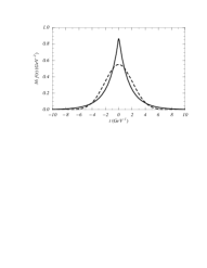
Figure 2: The perturbative short-distance function $f(t)$ for $m=5$ GeV and $\alpha_{s}=0.39$ (solid line) and the leading term in the delocalized multipole expansion of $f(t)$ for $\Omega=k^{2}/m$ (dashed line).

In Fig. 2 the function $f(t)$ (solid line) is displayed for $m=5$ GeV and $\alpha_{s}=0.39$. Since the spatial extension of the quarkonium system is neglected and the average time between interactions with the vacuum is of the order of the inverse kinetic energy, the characteristic width of $f$ is of order $(mv^{2})^{-1}\sim(m\alpha_{s}^{2})^{-1}$. As a comparison we have also displayed the function $[\int dt^{\prime}f(t^{\prime})\tilde{e}_{0}^{\Omega}(t^{\prime})]e_{0}^{\Omega}(t)$ for $\Omega=k^{2}/m$ (dashed line), which is the leading term in the delocalized multipole expansion of $f$. The values of the first few local multipole moments $f_{n}(\infty)$, which correspond to the local Wilson coefficients, read

$$\begin{array}[]{ll}f_{0}(\infty)\,=\,1.6518\,\frac{m}{36\,k^{4}}\,,&f_{2}(\infty)\,=\,1.3130\,\frac{m^{3}}{36\,k^{8}}\,,\\[8.53581pt] f_{4}(\infty)\,=\,7.7570\,\frac{m^{5}}{36\,k^{12}}\,,&f_{6}(\infty)\,=\,130.492\,\frac{m^{7}}{36\,k^{16}}\,,\\[8.53581pt] f_{8}(\infty)\,=\,4474.1\,\frac{m^{9}}{36\,k^{20}}\,,&f_{10}(\infty)\,=\,262709.3\,\frac{m^{11}}{36\,k^{24}}\,,\ldots\,.\end{array}$$ (41)

The term $f_{0}(\infty)$ agrees with Ref. [15, 16] and $f_{2}(\infty)$ with Ref. [18]. The results for $f_{n>2}(\infty)$ are new. Analytical expressions for the numbers shown in Eqs. (41) are given in App. B.

Let us compare the local expansion of $E^{np}$ with the resolution-dependent expansion using the basis functions of Eq. (11). For the nonperturbative gluonic field strength correlator we use a lattice inspired model of the form

$$g(t) = 12\,A_{0}\,\exp\Big{(}-\sqrt{t^{2}+\lambda_{A}^{2}}/\lambda_{A}+1\Big{)}\,,$$

$$A_{0} = 0.04~{}\mbox{GeV}^{4}\,,\qquad\lambda_{A}^{-1}\,=\,0.7~{}\mbox{GeV}\,,$$ (42)

This model has an exponential large-time behavior according to Eq. (32) and a smooth behavior for small $t$. The local dimension $4$ gluon condensate in this model is

$$\Big{\langle}\frac{\alpha_{s}}{\pi}\,G_{\mu\nu}^{a}G_{\mu\nu}^{a}\Big{\rangle}\,=\,\frac{6\,A_{0}}{\pi^{2}}\,=\,0.024\,\,\mbox{GeV}^{4}\,.$$ (43)

We note that for the purpose of this examination the exact form of the model for the nonperturbative gluonic field strength correlator is not an important issue as long as the derivatives of $g(t)$ at $t=0$ are well defined, see e.g. Refs. [6, 19] for different choices of models.

In Tab. 1 we have displayed the exact result in the model (42) and the first four terms of the resolution-dependent expansion of $E^{np}$ for the quark masses $m=5,25,45,90,175$ GeV and for $\Omega=\infty$ and $\Omega=k^{2}/m$. For each value of the quark mass the strong coupling has been fixed by the relation $\alpha_{s}=\alpha_{s}(k)$.

					$\Omega=\infty$		$\Omega=k^{2}/m$
$m$		$k^{2}/m$	$E^{np}$		$f_{n}g_{n}$	$\sum^{n}_{i=0}f_{i}g_{i}$	$f_{n}g_{n}$	$\sum^{n}_{i=0}f_{i}g_{i}$
(GeV)	$\alpha_{s}$	(MeV)	(MeV)	$n$	(MeV)	(MeV)	(MeV)	(MeV)
$5$	$0.39$	$0.338$	$24.8$	0	$38.6$	$38.6$	$24.2$	$24.2$
				2	$-65.7$	$-27.2$	$-3.9$	$20.3$
				4	$832.7$	$805.5$	$12.1$	$32.4$
				6	$-35048.0$	$-34242.4$	$-43.1$	$-10.8$
$25$	$0.23$	$0.588$	$12.6$	0	$16.0$	$16.0$	$12.8$	$12.8$
				2	$-9.0$	$7.0$	$-1.2$	$11.5$
				4	$37.8$	$44.8$	$2.6$	$14.1$
				6	$-526.6$	$-481.8$	$-6.7$	$7.4$
$45$	$0.19$	$0.722$	$4.9$	0	$5.9$	$5.9$	$5.0$	$5.0$
				2	$-2.2$	$3.7$	$-0.4$	$4.6$
				4	$6.1$	$9.8$	$0.7$	$5.3$
				6	$-56.4$	$-46.6$	$-1.4$	$3.8$
$90$	$0.17$	$1.156$	$1.05$	0	$1.15$	$1.15$	$1.07$	$1.07$
				2	$-0.17$	$0.98$	$-0.04$	$1.02$
				4	$0.18$	$1.16$	$0.04$	$1.07$
				6	$-0.65$	$0.51$	$-0.07$	$1.00$
$175$	$0.15$	$1.750$	$0.245$	0	$0.258$	$0.258$	$0.249$	$0.249$
				2	$-0.016$	$0.242$	$-0.005$	$0.244$
				4	$0.008$	$0.250$	$0.003$	$0.247$
				6	$-0.012$	$0.237$	$-0.003$	$0.244$

Table 1: Nonperturbative corrections to the heavy quarkonium ground state level at leading order in the multipole expansion with respect to the scales $m$, $mv$ and $mv^{2}$ for various quark masses $m$ based on the model in Eq. (42). Displayed are the exact result and the first few orders in the DOE for $\Omega=\infty$ and $\Omega=k^{2}/m$. The numbers are rounded off to units of $0.1$, $0.01$ or $0.001$ MeV.

We note that the series are all asymptotic, i.e.  they are not convergent for any resolution. The local expansion ($\Omega=\infty$) is quite badly behaved for smaller quark masses because for $k^{2}/m\mathrel{\raise 1.29167pt\hbox{$<$\kern-7.5pt\lower 4.30554pt\hbox{$\sim$}}}\lambda_{A}^{-1}$ any local expansion is meaningless. In particular, for $m=5$ GeV the subleading dimension $6$ term is already larger than the parametrically leading dimension $4$ term. This is consistent with the size of the dimension $6$ term based on a phenomenological estimate of the local dimension $6$ condensate in Eq. (36), see App. A. For quark masses, where $k^{2}/m\mathrel{\raise 1.29167pt\hbox{$>$\kern-7.5pt\lower 4.30554pt\hbox{$\sim$}}}\lambda_{A}^{-1}$, the local expansion is reasonably good. However, for finite resolution $\Omega=k^{2}/m$, the size of higher order terms is considerably smaller than in the local expansion for all quark masses, and the series appears to be much better behaved. The size of the order $n$ term is suppressed by approximately a factor $2^{-n}$ as compared to the order $n$ term in the local expansion. We find explicitly that terms in the series with larger $n$ decrease more quickly for finite resolution scale as compared to the local expansion. One also observes that even in the case $k^{2}/m<\lambda_{A}^{-1}$, where the leading term of the local expansion overestimates the exact result, the leading term in the delocalized expansion for $\Omega=k^{2}/m$ agrees with the exact result within a few percent. It is intuitively clear that this feature is a general property of the delocalized expansion, and we believe that it should apply to any problem for which the local expansion in the ratio of two scales breaks down because the ratio is not sufficiently small.

We would like to emphasize again that the previous analysis is not intended to provide a phenomenological determination of nonperturbative corrections to the heavy quarkonium ground state energy level, but rather to demonstrate the DOE within a specific model. For a realistic treatment of the nonperturbative contributions in the heavy quarkonium spectrum a model-independent analysis should be carried out. In addition, also higher orders in the local multipole expansion with respect to the ratios of scales $m$, $mv$ and $mv^{2}$ should be taken into account, which have been neglected here. These corrections might be substantial, in particular for smaller quark masses. However, having in mind an application to the bottomonium spectrum, we believe that our results for the expansion in $\Lambda/mv^{2}$ indicate that going beyond the leading term in the OPE for the bottomonium ground state is probably meaningless and that calculations based on the DOE with a suitable choice of resolution should be more reliable.

5 Extraction of the running gluon condensate

The resolution-dependent condensates are either determined phenomenologically from experimental data or from lattice measurements. It is the purpose of this section to extract the resolution-dependent dimension $4$ condensate from an analysis of moment ratios for the charmonium system and a sum rule for the Adler function using the $V+A$ spectral function measured at LEP in hadronic tau decays. In contrast to the demonstration in the previous section, where within our approximation, the vacuum was probed only by the temporal dynamics of the heavy quarkonium system, the charmonium moments and the $V+A$ sum rules probe the full four-dimensional space-time structure of the vacuum. We use the $4$-dimensional version of the DOE with a common resolution scale for each coordinate as given in Eqs. (25)–(28). For convenience we define

$$\Big{\langle}\frac{\alpha_{s}}{\pi}\,G^{2}\Big{\rangle}(\Omega)\,\equiv\,\frac{1}{2\pi^{2}}\,g_{0000}(\Omega)\,,$$ (44)

and in the following we will refer to it as the “running gluon condensate”. For $\Omega=\infty$ the running gluon condensate coincides with the local gluon condensate $\langle(\alpha_{s}/\pi)G^{a}_{\rho\sigma}(0)G^{a}_{\rho\sigma}(0)\rangle$.

5.1 Charmonium sum rules

The determination of the local gluon condensate $\Big{\langle}\frac{\alpha_{s}}{\pi}\,G^{2}\Big{\rangle}(\infty)$ from charmonium sum rules was pioneered in Refs. [20]. By now there is a vast literature on computations of Wilson coefficients to various loop-orders and various dimensions of the power corrections in the correlator of two heavy quark currents including updated analyses of the corresponding sum rules (see e.g. Refs. [21, 22]). Because the short-distance coefficient of the running gluon condensate is $\Omega$-independent, we can use the same strategy as in previous analyses, where the local condensate was determined. The only difference is that we have to keep track of its dependence on the characteristic short-distance scale.

The relevant correlator is

$$(q_{\mu}q_{\nu}-q^{2}\,g_{\mu\nu})\,\Pi^{c}(Q^{2})\,=\,i\int d^{4}x\,\mbox{e}^{iqx}\left\langle Tj^{c}_{\mu}(x)j^{c}_{\nu}(0)\right\rangle\,,\qquad Q^{2}=-q^{2}\,,$$ (45)

where $j_{\mu}\equiv\bar{c}\gamma_{\mu}c$, and the $n$-th moment is defined as

$${\cal M}_{n}\,=\,\frac{1}{n!}\,\left.\Big{(}\!-\frac{d}{dQ^{2}}\Big{)}^{n}\,\Pi^{c}(Q^{2})\,\right|_{Q^{2}=0}\,.$$ (46)

Assuming analyticity of $\Pi^{c}$ in $Q^{2}$ away from the negative, real axis and employing the optical theorem, the $n$th moment can be expressed as a dispersion integral over the charm pair cross section in $e^{+}e^{-}$ annihilation,

$${\cal M}_{n}\,=\,\frac{1}{12\pi^{2}\,Q_{c}^{2}}\,\int\frac{ds}{s^{n+1}}\,\frac{\sigma_{e^{+}e^{-}\to c\bar{c}+X}(s)}{\sigma_{e^{+}e^{-}\to\mu^{+}\mu^{-}}(s)}\,,$$ (47)

where $s$ is the square of the c.m. energy and $Q_{c}=2/3$. We consider the ratio [20]

$$r_{n}\,\equiv\,\frac{{\cal M}_{n}}{{\cal M}_{n-1}}$$ (48)

and extract the running gluon condensate as a function of $n$ from the equality of the theoretical ratio using Eq. (46) and the ratio based on Eq. (47) determined from experimental data.

The analytic form of the $n$-th moment in the local OPE up to terms with dimension $6$ reads [21]

$${\cal M}_{n} = \frac{3}{4\pi^{2}}\frac{2^{n}(n+1)(n-1)!}{(2n+3)!!}\,\frac{1}{(4m_{c}^{2})^{n}}\,\bigg{\{}\,1\,+\,\mbox{[pert. corrections]}$$

$$\hskip 28.45274pt\,+\,\delta^{(4)}_{n}\,\langle g^{2}G^{2}\rangle\,+\,\Big{[}\,\delta^{(6)}_{G,n}\,\langle g^{3}fG^{3}\rangle\,+\,\delta^{(6)}_{j,n}\,\langle g^{4}j^{2}\rangle\,\Big{]}\,+\,\ldots\,\bigg{\}}\,,$$

$$\delta^{(4)}_{n} = -\frac{(n+3)!}{(n-1)!\,(2n+5)}\,\frac{1}{9\,(4m_{c}^{2})^{2}}\,,$$

$$\delta^{(6)}_{G,n} = \frac{2}{45}\frac{(n+4)!\,(3n^{2}+8n-5)}{(n-1)!\,(2n+5)\,(2n+7)}\,\frac{1}{9\,(4m_{c}^{2})^{3}}\,,$$

$$\delta^{(6)}_{j,n} = -\frac{8}{135}\,\frac{(n+2)!\,(n+4)\,(3n^{3}+47n^{2}+244n+405)}{(n-1)!\,(2n+5)\,(2n+7)}\,\frac{1}{9\,(4m_{c}^{2})^{3}}\,,$$ (49)

where $\langle g^{3}fG^{3}\rangle\equiv\langle g^{3}f^{abc}G^{a}_{\mu\nu}G^{b}_{\nu\lambda}G^{c}_{\lambda\mu}\rangle$ and $\langle g^{4}j^{2}\rangle\equiv\langle g^{4}j^{a}_{\mu}j^{a}_{\mu}\rangle$, $j^{a}_{\mu}$ being the light flavor singlet current.

In contrast to the calculation of the quarkonium energy level in Sec. 4, where we had a nonrelativistic powercounting argument allowing for consistently considering only two gluons interacting with the vacuum, the local OPE of the charmonium moments is inconsistent if only the interaction of two gluons with the vacuum is accounted for. This is because the Wilson coefficients for condensates of dimension $6$ and higher are only gauge-invariant if the interaction of any number of gluons that can contribute at a certain dimension is taken into account. [21] Therefore, a reliable extraction of the running gluon condensate is only possible if the higher dimensional local terms summed in $\delta^{(4)}_{n}\langle g^{2}G^{2}\rangle(\Omega)$ represent a reasonably good approximation to the full set of terms with the corresponding dimensions in the local OPE. The most important subleading contributions in the local OPE are the dimension $6$ terms shown in Eq. (49). Using relation (65), one can derive that

$$\langle g^{2}GD^{2}G\rangle\,\equiv\,\langle g^{2}G_{\mu\nu}(0)\,D_{\rho}D_{\rho}\,G_{\mu\nu}(0)\rangle\,=\,2\,\langle g^{4}j^{2}\rangle\,-\,2\,\langle g^{3}fG^{3}\rangle\,.$$ (50)

Assuming further Eq. (34), then the local dimension $6$ contribution contained in $\delta^{(4)}\langle g^{2}G^{2}\rangle(\Omega)$ reads

$$\frac{1}{4\Omega^{2}}\,\delta^{(4)}_{n}\,\langle g^{2}GD^{2}G\rangle$$ (51)

In Tab. 2 we have displayed, for $\Omega=2m_{c}/n$, the ratio of the sum of local dimension $6$ contributions in the running gluon condensate correction according to Eq. (51) and the sum of the local dimension $6$ term in Eq. (49) for $r_{n}$. We have used the standard values $\langle g^{3}fG^{2}\rangle=0.045\,\,\mbox{GeV}^{6}$ obtained from the instanton gas approximation [1] and $\langle g^{4}j^{2}\rangle=-\rho\,4/3(4\pi)^{2}\alpha_{s}^{2}\langle\bar{q}q\rangle^{2}$ with $\alpha_{s}=0.7$ ($\mu\approx 0.7$ GeV) and $\langle\bar{q}q\rangle=-(0.24\,\,\mbox{GeV})^{3}$. The choice $\rho=1$ corresponds to exact vacuum saturation. As explained later we believe that $\Omega=2m_{c}/n$ is an appropriate choice for the resolution scale.

$n$	1	2	3	4	5	6	7	8
$\rho=1$	0.13	0.36	0.56	0.73	0.87	0.99	1.08	1.16
$\rho=2$	0.09	0.25	0.42	0.57	0.69	0.80	0.89	0.97

Table 2: Ratio of the local dimension-$6$ contributions contained in the running gluon condensate and in the full OPE for $r_{n}$ as a function of $n$.

Indeed, one finds for the relevant ratios $r_{n}$ ($2<n\mathrel{\raise 1.29167pt\hbox{$<$\kern-7.5pt\lower 4.30554pt\hbox{$\sim$}}}7$) that the local dimension $6$ contribution contained in the running gluon condensate has the same sign and roughly the same size as the dimension $6$ power correction in the full OPE for larger $n$, where higher dimensional contributions are more important.

For the experimental moments we use the compilation presented in Ref. [23], where the spectral function is split into contributions from the charmonium resonances, the charm threshold region, and the continuum. For the latter the authors of Ref. [23] used perturbation theory since no experimental data are available for the continuum region. We have assigned a 10% error for the spectral function in the continuum region. We believe that this is sufficiently conservative since a large part of the error drops out in the ratio $r_{n}$. For the purely perturbative contribution of the theoretical moments we used the compilation of analytic ${\cal O}(\alpha_{s}^{2})$ results from Ref. [23] and adopted the $\overline{\mbox{MS}}$ mass definition $\overline{m}_{c}(\overline{m}_{c})$ (for any renormalization scale $\mu$). For the Wilson coefficient of the gluon condensate we have used the expression given in Eqs. (49). We have checked that for $n\leq 8$ the perturbative ${\cal O}(\alpha_{s}^{2})$ corrections do not exceed 50% of the ${\cal O}(\alpha_{s})$ corrections for $\mu$ between $1$ and $4$ GeV.

Our result for the running gluon condensate as a function of $n$ is shown in Fig. 3 for $n\leq 8$ and $\overline{m}_{c}(\overline{m}_{c})=1.23$ (white triangles), $1.24$ (black stars), $1.25$ (white squares) and $1.26$ GeV (black triangles). For each value of $\overline{m}_{c}(\overline{m}_{c})$ and $n$ the area between the upper and lower symbols represents the uncertainty due to the experimental errors of the moments and variations of $\alpha_{s}(M_{Z})$ between $0.116$ and $0.120$ and of $\mu$ between $1$ and $3$ GeV.

Figure 3: The running gluon condensate as a function of $n$ when extracted from the ratio of moments $r_{n}$ for $\overline{m}_{c}(\overline{m}_{c})=1.23$ (white triangles), $1.24$ (black stars), $1.25$ (white squares) and $1.26$ GeV (black triangles). The area between the upper and lower symbols represents the uncertainties. The thick solid line indicates the running gluon condensate as it is obtained from the lattice-inspired ansatz in Eqs. (32)

We see that the running gluon condensate appears to be a decreasing function of $n$. Let us compare this behavior of the running gluon condensate with the one obtained from the lattice-inspired exponential ansatz for $g(x)$ in Eq. (32) using the definition of Eq. (16),

$$\Big{\langle}\frac{\alpha_{s}}{\pi}G^{2}\Big{\rangle}_{\rm lat}(\Omega)\,=\,\frac{6\,A_{0}}{\pi^{2}}\,\bigg{\{}\,1\,+\,\frac{1}{4\,\Omega^{2}\,\lambda_{A}^{2}}$$ (52)

$$\qquad-\,\frac{3\,\sqrt{\pi}}{4\,\Omega\,\lambda_{A}}\,\bigg{(}1+\frac{1}{6\,\Omega^{2}\,\lambda_{A}^{2}}\bigg{)}\,\mbox{e}^{1/(4\,\Omega^{2}\,\lambda_{A}^{2})}\,\bigg{(}\,1-{\rm erf}\Big{(}\frac{1}{2\,\Omega\,\lambda_{A}}\Big{)}\,\bigg{)}\,\bigg{\}}\,.\qquad$$

Here, ${\rm erf}$ is the error function. Due to the exponential behavior of the lattice-inspired ansatz for $g(x)$ the expression in Eq. (52) is a monotonic increasing function of $\Omega$. Since the exact width of the short-distance function $f$ for the moments is unknown we estimate it using physical arguments. For large $n$, i.e.  in the nonrelativistic regime, the width is of the order of the quark c.m. kinetic energy $mv^{2}$, which scales like $m/n$ because the average quark velocity in the $n$-th moment scales like $1/\sqrt{n}$. [24] For small $n$, on the other hand, the relevant short-distance scale is just the quark mass. Therefore, we take $\Omega=2m_{c}/n$ as the most appropriate choice of the resolution scale. In Fig. 3 the running gluon condensate from Eq. (52) is displayed for $\lambda_{A}^{-1}=0.7$ GeV and, exemplarily, $A_{0}=0.04$ (i.e. $\langle(\alpha_{s}/\pi)G^{2}\rangle_{\rm lat}(\infty)=0.024\,\,\mbox{GeV}^{4}$) and for $\Omega=(2.5\,\,\mbox{GeV})/n$ as the thick solid line. We find that the $n$-dependence of the lattice inspired running gluon condensate and our fit result from the charmonium sum rules are consistent. This appears to confirm the lattice result for the correlation length $\lambda_{A}$. However, the uncertainties of our extraction are still quite large, particularly for $n=2$, where the sensitivity to the error in the continuum region is enhanced. We also note that the values for the running gluon condensate tend to decrease with increasing charm quark mass. For $\overline{m}_{c}(\overline{m}_{c})=1.27$ GeV we find that $\langle(\alpha_{s}/\pi)G^{2}\rangle$ ranges from $-0.01\,\,\mbox{GeV}^{4}$ to $+0.01\,\,\mbox{GeV}^{4}$ and shifts further towards negative values for $\overline{m}_{c}(\overline{m}_{c})\mathrel{\raise 1.29167pt\hbox{$>$\kern-7.5pt\lower 4.30554pt\hbox{$\sim$}}}1.28$ GeV for all $n>2$. Assuming the reliability of the DOE as well as the local OPE in describing the nonperturbative effects in the charmonium sum rules and that the Euclidean scalar functions $D(x)$ and $D_{1}(x)$ in Eqs. (31)) are positive definite, our result disfavors $\overline{m}_{c}(\overline{m}_{c})\mathrel{\raise 1.29167pt\hbox{$>$\kern-7.5pt\lower 4.30554pt\hbox{$\sim$}}}1.28$ GeV.

5.2 $V+A$ sum rule

Recently, the spectral function for light quark production in the $V+A$ channel has been remeasured by the Aleph [25] and Opal [26] collaborations from hadronic $\tau$ decays for $q^{2}\leq m_{\tau}^{2}$. In the OPE the associated current correlator is dominated by the gluon condensate, and the dimension $6$ power corrections that are not due to a double covariant derivative in the local gluon condensate are suppressed. The corresponding currents are $j_{\mu}^{L/R}=\bar{u}\gamma_{\mu}(1\pm\gamma_{5})d$ and the relevant correlator in the chiral limit reads

$$i\int d^{4}\!x\,\mbox{e}^{iqx}\left\langle Tj_{\mu}^{L}(x)j_{\nu}^{R}(0)\right\rangle\,=\,(q_{\mu}q_{\nu}-q^{2}g_{\mu\nu})\,\Pi^{\rm V+A}(Q^{2})\,,\qquad Q^{2}=-q^{2}\,.$$ (53)

Up to ${\cal O}(\alpha_{s}^{3})$ the perturbative spectral function is given as [27]

$$\mbox{Im}\,\Pi^{\rm V+A}_{\rm pert}(-q^{2}-i\epsilon) = \frac{1}{2\pi}\,\bigg{(}\,1\,+\,\frac{\alpha_{s}(q^{2})}{\pi}\,+\,F_{3}\,\Big{(}\frac{\alpha_{s}(q^{2})}{\pi}\Big{)}^{2}\,+\,F_{4}\,\Big{(}\frac{\alpha_{s}(q^{2})}{\pi}\Big{)}^{3}+\ldots\bigg{)}\,,$$

$$F_{3} = 1.9857-0.1153\,n_{\ell}\,,$$

$$F_{4} = -6.6368-1.2001\,n_{\ell}-0.0052\,n^{2}_{\ell}\,,$$ (54)

where $n_{\ell}=3$ is the number of light quark flavors. The Wilson coefficient of the dimension-$4$ gluon condensate correction is known to order $\alpha_{s}$,

$$\Pi^{\rm V+A}_{\rm np}(Q^{2})\,=\,\frac{1}{6\,Q^{4}}\,\bigg{(}\,1-\frac{11}{18}\frac{\alpha_{s}}{\pi}\,\bigg{)}\,\Big{\langle}\frac{\alpha_{s}}{\pi}G^{2}\Big{\rangle}\,+\,\ldots\,.$$ (55)

Since the correlator $\Pi(Q^{2})^{\rm V+A}$ is cutoff-dependent itself, we investigate the Adler function

$$D(Q^{2})\,\equiv\,-Q^{2}\,\frac{\partial\,\Pi^{\rm V+A}(Q^{2})}{\partial\,Q^{2}}\,=\,\frac{Q^{2}}{\pi}\,\int_{0}^{\infty}ds\,\frac{\mbox{Im}\,\Pi^{\rm V+A}(s)}{(s+Q^{2})^{2}}\,.$$ (56)

For the corresponding experimental V+A spectral function we have used the Aleph measurement [25] in the resonance region up to $2.2$ GeV². For the continuum region above $2.2$ GeV² we used 3-loop perturbation theory for $\alpha_{s}(M_{Z})=0.118$, and we have set the renormalization scale $\mu$ to $Q$. We note that the pion pole of the axial vector contribution has to be taken into account in order to yield a consistent description in terms of the OPE for asymptotically large $Q$. [28] We have checked that the known perturbative contributions to the Adler function show good convergence properties. For $Q$ between $1.0$ and $2.0$ GeV and setting $\mu=Q$, the 3-loop (two-loop) corrections amount to $5\%$ ($7\%$) and $0.5\%$ ($1.4\%$), respectively. On the other hand, the ${\cal O}(\alpha_{s})$ correction to the Wilson coefficient of the gluon condensate are between $-16\%$ and $-6\%$ for $\mu$ between $0.8$ and $2.0$ GeV. In analogy to the analysis for charmonium sum rules and setting $\Omega=Q$ we have compared the local dimension $6$ contributions contained in the running gluon condensate in Eq. (55) with the sum of all dimension $6$ terms in the OPE as they were determined in Ref. [28]. The latter consist of local four-quark condensates, which we have estimated by assuming vacuum saturation at the scale $\mu\approx 0.7$ and using the parameters employed for the charmonium sum rules. We again found that the corresponding dimension $6$ contributions have equal sign and roughly the same size.

Our result for the running gluon condensate as a function of $Q$ is shown in Fig. 4.

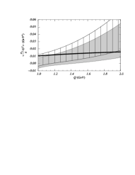
Figure 4: The running gluon condensate as a function of $Q$ when extracted from the Adler function. The grey area represents the allowed region using perturbation theory at ${\cal O}(\alpha_{s}^{3})$ and the striped region using perturbation theory at ${\cal O}(\alpha_{s}^{2})$. The thick solid line denotes the running gluon condensate from the lattice-inspired ansatz in Eqs. (32) for $\Omega=Q$.

for $1$ GeV$\leq Q\leq 2$ GeV. The shaded region represents the allowed range obtained from an analysis employing the full ${\cal O}(\alpha_{s}^{3})$ perturbative contribution and the striped region is obtained at ${\cal O}(\alpha_{s}^{2})$. The uncertainties are due to the experimental errors in the spectral function and a variation of the renormalization scale $\mu$ in the range $Q\pm 0.25$ GeV. The strong coupling has been fixed at $\alpha_{s}(M_{Z})=0.118$. We have restricted our analysis to the range $1\,\,\mbox{GeV}<Q<2\,\,\mbox{GeV}$ because for $Q\mathrel{\raise 1.29167pt\hbox{$<$\kern-7.5pt\lower 4.30554pt\hbox{$\sim$}}}1$ GeV perturbation theory becomes unreliable and for $Q\mathrel{\raise 1.29167pt\hbox{$>$\kern-7.5pt\lower 4.30554pt\hbox{$\sim$}}}2$ GeV the experimentally unknown part of the spectral function at $s\geq 2.2$ GeV² is being probed. The thick black line in Fig. 4 shows the lattice-inspired running gluon condensate of Eq. (52) for $\Omega=Q$ using the parameters from Sec. 5.1. We find that our result for the running gluon condensate as a function of $Q$ is consistent with a function that increases with $Q$. The result is also consistent with the lattice-inspired expression for the running gluon condensate, but the uncertainties of our extraction are too large and the running of the lattice-inspired condensate in the range between $1$ and $2$ GeV is too small to draw a more definite conclusion.

6 Anomalous dimensions

In the previous sections we have presented the formalism for the DOE assuming that the separation of fluctuations at different length scales can be carried out without ambiguities and that there is no need to introduce a regularization scheme. We have applied the DOE for QCD quantities, where nonperturbative effects are dominated by the gluon condensate, which can be defined such that its anomalous dimension vanishes to all orders. This allowed us to ignore anomalous dimensions at the level of precision intended in our investigations in Sec. 5.

However, in general, the separation of fluctuations at different length scales is ambiguous and a regularization scheme is required to carry out the separation systematically. In this general case, the delocalized condensates cannot be defined through the integrals in Eqs. (16) or (27) because the resolution scale $\Omega$ would itself serve as a UV-regulator and, therefore, interfere with the regularization scheme. Since the regularization of the short-distance coefficients in the DOE remains unaffected, this would lead to inconsistencies in the DOE. Thus, in the general case, the delocalized condensates are defined through the sum over local condensates given in Eq. (20) (and its $d$-dimensional generalization), which should be considered more fundamental than Eqs. (16) and (27). We emphasize that with this definition there is, by construction, no interference between the DOE and the regularization scheme. Having in mind perturbative computations in quantum field theories in general, this means in particular that the delocalized expansion does – up to the summations that define the short-distance coefficients and the matrix elements – not affect renormalization, i.e.  the structure of anomalous dimensions, the running of coefficients and matrix elements, etc..

Coming back to the lattice-inspired expression for the running gluon condensate in Eq. (52) it is now clear that it was determined in the exponential cutoff scheme defined through Eq. (27). However, because the $\Omega$-dependence of the running gluon condensate is mainly due to the exponential behavior of $g(x)$ and because the actual renormalization-scale-dependence of the running gluon condensate is small (due to the fact that it is generated by local condensates of dimension $6$ and higher) the use of expression (52) for the comparisons in Sec. 5, where the perturbative contributions were determined in the $\overline{\mbox{MS}}$ scheme, are justified.

It is obvious that the delocalized expansion can in principle be applied to any quantum field theoretical computation, where a local expansion can be carried out. In particular, it can be applied in effective theories, and it allows for the systematic summation of matrix elements of operators with additional covariant derivatives in addition to the summation of large logarithmic perturbative corrections obtained from solving the renormalization group equations for the short-distance coefficients. In the following we briefly demonstrate the delocalized expansion in the presence of a regularization scheme – dimensional regularization to be specific – for $f_{D}/f_{B}$ at leading order in the heavy quark mass expansion.

The meson decay constants are an important parameter in computations of mixing and lifetime-differences. They can be computed in heavy quark effective theory (HQET) in an expansion in $\Lambda_{\rm QCD}/m_{Q}$, where $m_{Q}$ is the respective heavy quark mass. To be definite, we consider the decay constant of a pseudoscalar meson, which is defined as

$$\langle 0|\bar{q}\,\gamma^{\mu}\,\gamma^{5}\,Q|P(v)\rangle\,=\,i\,f_{P}\,\sqrt{M_{P}}\,v^{\mu}\,,$$ (57)

where $q$ and $Q$ are the light and heavy quark fields in full QCD, $P(v)$ is the meson state with velocity $v$ in full QCD, and $M_{P}$ is the mesons mass. In the (local) $1/m_{Q}$-expansion the current $\bar{q}\gamma^{\mu}\gamma^{5}Q$ is written as a series of HQET currents of increasing dimension each of which is multiplied by a Wilson coefficient:

$$\bar{q}\gamma^{\mu}\gamma^{5}Q\,\to\,-\,C_{0}(m_{Q},\mu)\,\bar{q}\gamma^{5}\gamma^{\mu}h_{Q}\,-\,C_{1}(m_{Q},\mu)\,\bar{q}\gamma^{5}v^{\mu}h_{Q}\,+\,\ldots\,.$$ (58)

Here, $h_{Q}$ denotes the heavy quark field in HQET and the ellipses represent contributions from currents with higher dimensions. The leading logarithmic expressions for the Wilson coefficients read [29]

$$C_{0}(m_{Q},\mu)\,=\,\bigg{(}\frac{\alpha_{s}(m_{Q})}{\alpha_{s}(\mu)}\bigg{)}^{-\frac{2}{\beta_{0}}}\,,\qquad C_{1}(m_{Q},\mu)\,=\,0\,,$$ (59)

where $\beta_{0}$ is the one-loop beta-function. Since the vacuum-to-meson matrix element of the current $\bar{q}\gamma^{5}\gamma^{\mu}h_{Q}$ is equal for $B$ and $D$ mesons at leading order in $1/m_{Q}$, this leads to the leading order relation

$$\frac{f_{D}}{f_{B}}\,=\,\sqrt{\frac{M_{B}}{M_{D}}}\,\bigg{(}\frac{\alpha_{s}(m_{b})}{\alpha_{s}(m_{c})}\bigg{)}^{\frac{6}{25}}$$ (60)

for $4$ active light flavors. Recent lattice measurements [30] indicate that

$$\frac{f_{D}}{f_{B}}\,\simeq\,\mbox{1.0 -- 1.3}\,,$$ (61)

but the RHS of Eq. (60) gives $f_{D}/f_{B}\approx 1.5$. It was found in Ref. [31] that the discrepancy cannot be accounted for quantitatively by subleading $1/m_{Q}$ contributions, because the corresponding corrections are simply too large to allow for a quantitative improvement of the leading order relation in Eq. (60). In particular, for the $D$ meson the local $1/m_{Q}$ expansion seems to break down, and it appears that going beyond the leading order approximation for $f_{D}/f_{B}$ is meaningless.

We suspect that the same statement might also apply to the delocalized version of the $1/m_{Q}$ expansion, but from the examinations in the previous parts of this paper one can expect that the delocalized expansion might provide a better leading order approximation for an appropriate choice of resolution scales. In the delocalized $1/m_{Q}$ expansion the leading order short-distance coefficients are equivalent to the local ones shown in Eq. (59). However, the vacuum-to-meson matrix element of the current $\bar{q}\gamma^{5}\gamma^{\mu}h_{Q}$ becomes a resolution-scale-dependent quantity because it sums matrix elements of local currents of the generic form $D^{2n}\bar{q}\gamma^{5}\gamma^{\mu}h_{Q}$ ($n\geq 0$). Evidently, the proper choice of the resolution scale is $\Omega\sim m_{Q}$. Thus the leading order expression for $f_{D}/f_{B}$ in the delocalized expansion can be written as

$$\frac{f_{D}}{f_{B}}\,=\,\sqrt{\frac{M_{B}}{M_{D}}}\,\bigg{(}\frac{\alpha_{s}(m_{b})}{\alpha_{s}(m_{c})}\bigg{)}^{\frac{6}{25}}\,\rho\,,$$ (62)

where

$$\rho\,=\,\frac{\langle 0|\bar{q}\,\gamma^{5}\gamma^{\mu}\,h_{c}|D(v)\rangle(\mu,\Omega=m_{c})}{\langle 0|\bar{q}\,\gamma^{5}\gamma^{\mu}\,h_{b}|B(v)\rangle(\mu,\Omega=m_{b})}\,.$$ (63)

The common renormalization scale $\mu$ in the $\Omega$-dependent matrix elements is set below the charm quark mass, but not fixed otherwise. Comparing expression (62) with the lattice result one finds $\rho\simeq\mbox{0.6--0.8}$. (Neglecting the anomalous dimension of the current $\bar{q}\gamma^{5}\gamma^{\mu}h_{Q}$ gives essentially the same result due to the large uncertainty of the lattice measurements.) We are not aware of any other independent determination of the ratio $\rho$, but this scaling relation has an interesting physical interpretation in the framework of a model, where one assumes that the $B$ and the $D$ meson wave functions have approximately the same size and that the vacuum-to-meson matrix elements of the local currents $D^{2n}\bar{q}\gamma^{5}\gamma^{\mu}h_{Q}$ scale like inverse powers of the meson size. Assuming exemplarily that the meson wave functions have a Gaussian drop-off behavior (see e.g. Ref. [33]) $\langle 0|\bar{q}(-\mathbf{x}/2)\gamma^{5}\gamma^{\mu}\,S(-\mathbf{x}/2,\mathbf{x}/2)\,h_{Q}(\mathbf{x}/2)|P\rangle\sim\exp(-|\mathbf{x}|^{2}/\lambda^{2})$ one finds, using the $3$-dimensional version of Eq. (27),

$$\rho\,\simeq\,\left(\,\frac{1+\frac{1}{\lambda^{2}m_{b}^{2}}}{1+\frac{1}{\lambda^{2}m_{c}^{2}}}\,\right)^{\frac{3}{2}}\,.$$ (64)

One can then derive that $\lambda^{-1}\simeq\mbox{0.5--0.8}$ GeV, which gives an estimate for the meson size. On the other hand, for an exponential drop-off behavior $\sim\exp(-|\mathbf{x}|/\lambda)$ one obtains $\lambda^{-1}\simeq\mbox{0.3--0.7}$ GeV.

7 Summary and outlook

In this paper we have proposed a new type of short-distance expansion of correlators of gauge invariant currents in QCD, which we name delocalized operator expansion (DOE). This expansion originates from nonlocal projections of gauge invariant correlation functions based on a delocalized version of the multipole expansion for the perturbatively calculable coefficient functions. Whereas the usual (local) OPE is based on a multipole expansion where the short-distance process in configuration space is written as the sum of delta-functions and derivatives of delta-functions, the DOE is based on a delocalized version of the multipole expansion using functions that have the width $\Omega^{-1}$. We call $\Omega$ the resolution parameter. In this paper we have constructed such a delocalized multipole expansion based on the Gaussian function and using the orthonormality and completeness properties of the Hermite polynomials. We emphasize that other, similar constructions are possible which have properties that are comparable to the one presented here and that they might be even better suited to certain problems than the one we have used here.

In the DOE the condensates become quantities that are dependent on the resolution parameter $\Omega$ and are related to an infinite sum of VEV’s of local operators with equal and larger number of covariant derivatives. The short-distance coefficients also become dependent on the resolution parameter $\Omega$ and are related to a finite sum of short-distance coefficients to local operators with equal and fewer number of covariant derivatives. The relative weight of the local terms in these sums is governed by the resolution parameter $\Omega$. For $\Omega\to\infty$ the DOE reduces to the usual local OPE. As is the local OPE, the DOE is parametrically an expansion in powers of $\Lambda/Q$, where $\Lambda$ denotes the highest nonperturbative scale occurring in the corresponding gauge invariant correlation function and $Q$ is the external short-distance scale at which the vacuum is being probed. If the resolution scale is chosen to be of order $Q$, there is an additional suppression of higher orders in the expansion by powers of a small number. This can be understood intuitively, because for $\Omega\sim Q$ the leading term in the delocalized multipole expansion represents a better approximation of the short-distance process than the delta-function. In this way the DOE can account for non-local effects.

Calculating the nonperturbative correction to the perturbatively determined ground state energy of a heavy quarkonium system, we have demonstrated the improved convergence properties of the delocalized expansion using a lattice-inspired toy model for the gluonic $2$-point field strength correlator. Reversing the situation, we have extracted the running gluon condensate $\langle(\alpha_{s}/\pi)G^{2}\rangle(\Omega)$ from experimental data using charmonium sum rules and the Adler function in the $V+A$ channel of light quark pair production. We found strong evidence that the gluon condensate is indeed a resolution-dependent quantity and our results are consistent with recent lattice measurements of the correlation length of the gluon field strength correlator.

The DOE can be applied in the framework of effective theories. By construction, the DOE does not interfere with the regularization scheme since the resolution-dependent short-distance coefficients and matrix elements are defined as sums of local short-distance coefficients and matrix elements, respectively. Thus, the DOE does not affect the renormalization properties of a theory. In the DOE we have derived the leading order expression for $f_{D}/f_{B}$ in the heavy quark mass expansion.

Further investigations and more detailed applications of the DOE are planned in forthcoming work.

Appendix A Tensor structure of $\langle g^{2}GD^{2}G\rangle$

Here we show that the lattice-implied dominance of the tensor structure in Eq. (34) for the gluon field strength correlator is consistent with a phenomenological determination of the dimension 6 condensate $\langle g^{2}G_{\mu\nu}(0)D_{\alpha}D_{\beta}G_{\kappa\lambda}(0)\rangle$. When evaluated in Schwinger gauge $x_{\mu}A_{\mu}=0$ [4] we are, according to Eq. (28), concerned with the quantity $\left\langle g^{2}G^{a}_{\mu\nu}\partial_{\rho}\partial_{\rho}G^{a}_{\alpha\beta}\right\rangle$ taken at $x=0$. Following Ref. [21] it can be parametrized in Euclidean space-time as

$$-\left\langle g^{2}G^{a}_{\mu\nu}\partial_{\rho}\partial_{\rho}G^{a}_{\alpha\beta}\right\rangle = 8\,O^{-}\left(\delta_{\mu\beta}\delta_{\alpha\nu}-\delta_{\mu\alpha}\delta_{\nu\beta}\right)$$ (65)

$$+\,O^{-}\left(\delta_{\mu\beta}\delta_{\alpha\nu}+\delta_{\alpha\nu}\delta_{\mu\beta}-\delta_{\alpha\mu}\delta_{\nu\beta}-\delta_{\beta\nu}\delta_{\mu\alpha}\right)$$

$$+\,O^{+}\left(\delta_{\mu\beta}\delta_{\alpha\nu}+\delta_{\mu\beta}\delta_{\alpha\nu}-\delta_{\mu\alpha}\delta_{\nu\beta}-\delta_{\nu\beta}\delta_{\mu\alpha}\right)\,,$$

where

$$O^{\pm}\,\equiv\,\frac{1}{72}\left\langle g^{4}j^{a}_{\mu}j^{a}_{\mu}\right\rangle\pm\frac{1}{48}\left\langle g^{3}f_{abc}G^{a}_{\mu\nu}G^{b}_{\nu\lambda}G^{c}_{\lambda_{\mu}}\right\rangle\,,$$ (66)

and $j^{a}_{\mu}$ denotes a light flavor-singlet current. In Eq. (65) the tensor structure multiplying $8\,O^{-}$ is the same as the one resulting from an omission of the terms involving $D_{1}$ in the parametrization of Eq. (31). Now, we consider

$$\left\langle g^{2}G^{a}_{\mu\nu}\partial_{\rho}\partial_{\rho}G^{a}_{\mu\nu}\right\rangle\,=\,96\,Q^{-}+24\,(O^{-}+O^{+})\,,$$ (67)

and we have to show that, phenomenologically, the contribution $96\,Q^{-}$ is the dominant one, that is

$$R_{O}\,\equiv\,\frac{96\,Q^{-}}{24\,(O^{-}+O^{+})}\,\gg\,1\,.$$ (68)

Assuming exact vacuum saturation to express $\left\langle g^{4}j^{2}\right\rangle$ in terms of a square of the quark condensate and using $\alpha_{s}=0.7$ ($\mu=0.7$ GeV), $\left\langle g^{3}f_{abc}G^{a}_{\mu\nu}G^{b}_{\nu\lambda}G^{c}_{\lambda\mu}\right\rangle=0.045$ GeV⁶, and $\langle\bar{q}q\rangle=-(0.24\,\,\mbox{GeV})^{3}$ as in Sec. 5.1, we obtain

$$\frac{\left\langle g^{3}f_{abc}G^{a}_{\mu\nu}G^{b}_{\nu\lambda}G^{c}_{\lambda\mu}\right\rangle}{\left\langle g^{4}j^{a}_{\mu}j^{a}_{\mu}\right\rangle}\,\sim\,-2.3\,.$$ (69)

For the ratio $R_{O}$ of Eq. (68) this implies

$$R_{O}\,\sim\,8.8\,,$$ (70)

which justifies the omission of the terms in the second and third line of Eq. (65).

Appendix B Short-distance coefficients for quarkonium ground states energy levels

$$f_{0}(\infty) = \frac{702}{425}\,\frac{m}{36\,k^{4}}\,,$$ (71)

$$f_{2}(\infty) = \frac{1108687904}{844421875}\,\frac{m^{3}}{36\,k^{8}}\,,$$ (72)

$$f_{4}(\infty) = \frac{17608502062304825344}{2270010244541015625}\,\frac{m^{5}}{36\,k^{12}}\,,$$ (73)

$$f_{6}(\infty) = \frac{45707850430207738594209974779904}{350274120613508115758056640625}\,\frac{m^{7}}{36\,k^{16}}\,,$$ (74)

$$f_{8}(\infty) = \frac{3377025742042031485195560438171693564080529866752}{754795366909616960779550333930811309814453125}\,\frac{m^{9}}{36\,k^{20}}\,.\quad\mbox{}$$ (75)

References

- [1] M. A. Shifman, A. I. Vainshtein and V. I. Zakharov, Nucl. Phys. B 147, 385 (1979). Nucl. Phys. B 147, 448 (1979).
- [2] P. M. Morse and H. Feshbach, Methods of Theoretical Physics, Part II, (McGraw-Hill Book Company, Inc., New York, 1953).
- [3] H. G. Dosch and Y. A. Simonov, Phys. Lett. B 205, 339 (1988).
- [4] J. Schwinger, Particles, Sources and Fields, Vol. I, Sec. 3.11, (Addison-Wesley Publishing Company, Inc., New York, 1970); A. V. Smilga, Sov. J. Nucl. Phys. 35, 271 (1982) [Yad. Fiz. 35, 473 (1982)].
- [5] K. G. Chetyrkin, V. P. Spiridonov and S. G. Gorishnii, Phys. Lett. B 160, 149 (1985); G. T. Loladze, L. R. Surguladze and F. V. Tkachov, Phys. Lett. B 162, 363 (1985).
- [6] D. Gromes, Phys. Lett. B 115, 482 (1982).
- [7] S. V. Mikhailov and A. V. Radyushkin, Sov. J. Nucl. Phys. 49, 494 (1989) [Yad. Fiz. 49, 794 (1988)]; Phys. Rev. D 45, 1754 (1992); A. P. Bakulev and S. V. Mikhailov, Phys. Rev. D 65, 114511 (2002) [arXiv:hep-ph/0203046].
- [8] A. V. Radyushkin, Phys. Lett. B 271, 218 (1991).
- [9] P. Ball, V. M. Braun and H. G. Dosch, Phys. Rev. D 44, 3567 (1991).
- [10] R. Hofmann, Phys. Lett. B 520, 257 (2001) [arXiv:hep-ph/0109007].
- [11] A. H. Mueller, Nucl. Phys. B 250, 327 (1985).
- [12] M. D’Elia, A. Di Giacomo and E. Meggiolaro, Phys. Lett. B 408, 315 (1997) [arXiv:hep-lat/9705032].
- [13] G. S. Bali, N. Brambilla and A. Vairo, Phys. Lett. B 421, 265 (1998) [arXiv:hep-lat/9709079].
- [14] M. B. Voloshin, Nucl. Phys. B 154, 365 (1979).
- [15] H. Leutwyler, Phys. Lett. B 98, 447 (1981).
- [16] M. B. Voloshin, Sov. J. Nucl. Phys. 35, 592 (1982) [Yad. Fiz. 35, 1016 (1982)]; Sov. J. Nucl. Phys. 36, 143 (1982) [Yad. Fiz. 36, 247 (1982)].
- [17] A. H. Hoang et al., Eur. Phys. J. directC 3, 1 (2000) [arXiv:hep-ph/0001286].
- [18] A. Pineda, Nucl. Phys. B 494, 213 (1997) [arXiv:hep-ph/9611388].
- [19] I. I. Balitsky, Nucl. Phys. B 254, 166 (1985).
- [20] V. A. Novikov, L. B. Okun, M. A. Shifman, A. I. Vainshtein, M. B. Voloshin and V. I. Zakharov, Phys. Rev. Lett. 38, 626 (1977) [Erratum-ibid. 38, 791 (1977)]; Phys. Lett. B 67, 409 (1977).
- [21] S. N. Nikolaev and A. V. Radyushkin, Nucl. Phys. B 213, 285 (1983).
- [22] S. N. Nikolaev and A. V. Radyushkin, Phys. Lett. B 124, 243 (1983).
- [23] J. H. Kuhn and M. Steinhauser, Nucl. Phys. B 619, 588 (2001) [arXiv:hep-ph/0109084].
- [24] A. H. Hoang, Phys. Rev. D 59, 014039 (1999) [arXiv:hep-ph/9803454].
- [25] R. Barate et al. [ALEPH Collaboration], Eur. Phys. J. C 4, 409 (1998).
- [26] K. Ackerstaff et al. [OPAL Collaboration], Eur. Phys. J. C 7, 571 (1999) [arXiv:hep-ex/9808019].
- [27] L. R. Surguladze and M. A. Samuel, Phys. Rev. Lett. 66, 560 (1991) [Erratum-ibid. 66, 2416 (1991)]; S. G. Gorishnii, A. L. Kataev and S. A. Larin, JETP Lett. 53, 127 (1991) [Pisma Zh. Eksp. Teor. Fiz. 53, 121 (1991)].
- [28] E. Braaten, S. Narison and A. Pich, Nucl. Phys. B 373, 581 (1992).
- [29] M. A. Shifman and M. B. Voloshin, Sov. J. Nucl. Phys. 45, 292 (1987) [Yad. Fiz. 45, 463 (1987)]; H. D. Politzer and M. B. Wise, Phys. Lett. B 206, 681 (1988).
- [30] S. M. Ryan, Nucl. Phys. Proc. Suppl. 106, 86 (2002) [arXiv:hep-lat/0111010].
- [31] M. Neubert, Phys. Rev. D 46, 1076 (1992).
- [32] T. A. DeGrand and R. D. Loft, Phys. Rev. D 38, 954 (1988).
- [33] D. S. Hwang and G. H. Kim, Phys. Rev. D 55, 6944 (1997) [arXiv:hep-ph/9601209].