QCD at non-zero chemical potential and temperature from the lattice

Abstract

A study of QCD at non-zero chemical potential, $\mu$, and temperature, $T$, is performed using the lattice technique. The transition temperature (between the confined and deconfined phases) is determined as a function of $\mu$ and is found to be in agreement with other work. In addition the variation of the pressure and energy density with $\mu$ is obtained for $\mu\,\hbox to0.0pt{\lower 3.5pt\hbox{$\mathchar 0\relax\sim$}\hss}\raise 1.0pt\hbox{$>$}\,0$. These results are of particular relevance for heavy-ion collision experiments.

1 Introduction

The QCD phase diagram has come under increasing experimental and theoretical scrutiny over the last few years. On the experimental side, very recent studies of compact astronomical objects have suggested that their cores contain “quark matter”, i.e. QCD in a new, unconfined phase where the basic units of matter are quarks, rather than nuclei or nucleons[1]. More terrestrially, heavy ion collision experiments, such as those performed at RHIC and CERN, are also believed to be probing unconfined QCD[2]. On the theoretical side, the study of QCD under these extreme densities and temperatures has proceeded along several fronts. One of the most promising areas of research is the use of lattice techniques to study either QCD itself, or model theories which mimic the strong interaction[3]. Clearly the most satisfying approach would be the former, i.e. a direct lattice study of QCD at various coordinates $(T,\mu)$ in its phase space ($\mu$ is the chemical potential for the quark number). However, until recently, this has proved intractable at a practical level for very fundamental reasons. This is because the Monte Carlo integration technique, which is at the heart of the (Euclidean) lattice approach, breaks down when $\mu\neq 0$. This work summarises one new approach which overcomes this problem and has made progress for $\mu\neq 0$ and $T\neq 0$.

In the next section a summary is given of the lattice technique and the problem incurred when $\mu\neq 0$. Section 3 describes the method used to overcome these difficulties and section 4 outlines the simulation details. The next two sections apply the method to variations in $m$ and $\mu$, and section 7 describes calculations of the pressure and energy density as functions of $\mu$.

A full account of this work is published elsewhere[4].

2 Lattice technique

On the lattice, the quark fields, $\psi(x)$, are defined on the sites, $x$, and the gluonic fields, $U_{\mu}(x)$, on the links $x\rightarrow x+\mu$. Observables are then calculated via a Monte Carlo integration approach:

$$<{\Omega}>\;\;=\;\;\frac{1}{N_{\{U,\psi,\bar{\psi}\}}}\sum_{\{U,\psi,\bar{\psi}\}}\ ^{\!\!\!\!\!\!\!\!{}^{\prime}}\;\;{\Omega}(\psi,\bar{\psi},U)$$ (1)

where $\sum^{\prime}$ represents a sum over configurations $\{U,\psi,\bar{\psi}\}$ which are selected with probability proportional to the Boltzmann weight $P(\{U,\psi,\bar{\psi}\})\propto e^{-S(\{U,\psi,\bar{\psi}\})}$ where $S$ is a suitably defined (Euclidean) gauge-invariant action. The fermionic part of this action is

$$S_{F}=\sum_{x}\bar{\psi}(x) \underbrace{(D\!\!\!\!/+m)} \psi(x).$$

$${=M}$$

For $\mu=0$ it can be shown that this action produces a (real-valued) positive Boltzmann weight.

Calculations at non-zero temperature, $T\neq 0$, can be performed by using a lattice with a finite temporal extent of $N_{t}a=1/T$, where $N_{t}$ is the number of lattice sites in the time dimension. In practice, $T$ is varied by changing the gauge coupling, $g_{0}$, and hence (through dimensional transmutation) the lattice spacing, $a$, rather than by changing $N_{t}$ (which can only be changed in discrete steps!).

The chemical potential is introduced into the system via an additional term in the quark matrix $M$, proportional to the Dirac matrix, $\gamma_{0}$,

$${M}\rightarrow{M}+\mu\gamma_{0}.$$ (3)

For $\mu\neq 0$, this leads to a complex-valued Boltzmann “weight” which can therefore no longer be used as a probability distribution, and, hence, the Monte Carlo integration procedure is no longer applicable. This is known as the Sign Problem and has plagued more than a decade of lattice calculations of QCD at $\mu\neq 0$.

3 Reweighting

This section outlines the Ferrenberg-Swendsen reweighting approach[5] which is used to overcome the sign problem detailed in the previous section. Observables at one set of parameter values $(\beta,m,\mu)$ (where $\beta=6/g_{0}^{2}$, and $m$ is the quark mass) can be calculated using an ensemble generated at another set of parameters $(\beta_{0},m_{0},\mu_{0})$ as follows,

$$\langle{\Omega}\rangle_{(\beta,m,\mu)} \equiv \frac{1}{{Z}(\beta,m,\mu)}\int{D}U{\Omega}\det M(m,\mu){\rm e}^{-S_{g}(\beta)}$$ (4)

$$= \frac{\left\langle{\Omega}\;{\rm e}^{(\ln\det M(m,\mu)-\ln\det M(m_{0},\mu_{0}))}{\rm e}^{-S_{g}(\beta)+S_{g}(\beta_{0})}\right\rangle_{(\beta_{0},m_{0},\mu_{0})}}{\left\langle{\rm e}^{(\ln\det M(m,\mu)-\ln\det M(m_{0},\mu_{0}))}{\rm e}^{-S_{g}(\beta)+S_{g}(\beta_{0})}\right\rangle_{(\beta_{0},m_{0},\mu_{0})}}.$$ (5)

Here $S_{g}$ is the gauge action.

In principle, Eq.(5) can be used to map out the entire phase diagram of QCD. However, it has been found that its naive application fails since the relative size of fluctuations in both numerator and denominator tend to grow exponentially with the volume of the system studied. This is a signal that the overlap between the ensemble at $(\beta_{0},m_{0},\mu_{0})$ is small compared with that at $(\beta,m,\mu)$.

One study which has had success in using Eq.(5) is that of Fodor and Katz[6]. They apply the reweighting approach not at an arbitrary point, $(T,\mu)$, in the phase diagram, but rather they trace out the phase transition line $T_{c}(\mu)$. This method is successful presumably because the overlap between the ensembles remains high along the “coexistence” line which defines the transition.

This paper utilises an alternative approach which Taylor expands Eq.(5) as a function of $\mu$ (or $m$) and hence estimates the derivatives of various quantities w.r.t. $\mu$ (or $m$). Derivatives up to the second order are considered, thus for $<\Omega>$ (in the case of a Taylor expansion in $\mu$) we have

$$\langle{\Omega}\rangle_{(\beta,\mu)}={\langle({\Omega}_{0}+{\Omega}_{1}\mu+{\Omega}_{2}\mu^{2})\exp({R}_{1}\mu+{R}_{2}\mu^{2}-\Delta S_{g})\rangle_{(\beta_{0},\mu_{0})}\over{\langle\exp({R}_{1}\mu+{R}_{2}\mu^{2}-\Delta S_{g})\rangle_{(\beta_{0},\mu_{0})}}},$$ (6)

where $\mu_{0}=0$. In Eq.(6), ${R}_{n}$ is the $n-$th derivative of the fermionic reweighting factor in Eq.(5), i.e.

$$\ln\left({{\det M(\mu)}\over{\det M(0)}}\right)=\sum_{n=1}^{\infty}\frac{\mu^{n}}{n!}\frac{\partial^{n}\ln\det M(0)}{\partial\mu^{n}}\equiv\sum_{n=1}^{\infty}{R}_{n}\mu^{n}.$$ (7)

The $\Omega_{n}$ are similarly the $n-$th derivatives of the observable $\Omega$.

Two observables are studied: the chiral condensate $<\overline{\psi}\psi>$ and the Polyakov Loop, $L$. Since $L$ is a pure gluonic quantity, defined as

$$<L>=<\frac{1}{V_{s}}\sum_{\vec{x}}Tr\prod_{t=0}^{N_{t}}U_{t}(\vec{x},t)>,$$ (8)

all of its derivatives are zero. (Here, $V_{s}$ is the spatial volume.) However, the expansion of $<\overline{\psi}\psi>$ is more challenging since it is defined as

$$\langle\bar{\psi}\psi\rangle\sim\langle{\rm tr}M^{-1}\rangle,$$ (9)

and hence the application of Eq.(6) requires determinations of $\partial^{n}M^{-1}/\partial\mu^{n}$.

The susceptibilities, $\chi$, of both $<\overline{\psi}\psi>$ and $L$ are defined as usual by their fluctuations, e.g.

$$\chi_{L}=\mbox{(volume factor)}\;\times\;(<L^{2}>-<L>^{2}).$$ (10)

These susceptibilities have a maximum at the transition point, $\beta_{c}$, and hence can be used to determine the transition point $\beta_{c}(m,\mu)$.

4 Simulation details

The lattice calculations were performed using a “p4-improved” discretisation of the continuum action which is a sophisticated lattice action maintaining rotational invariance of the free fermion propagator up to $O(p^{4})$ [7, 8] ($p$ is the momentum here). Two dynamical flavours of quarks were used with a $16^{3}\times 4$ lattice. Simulations were performed at quark mass, $m=0.1$ and $0.2$ which correspond to (unphysically heavy) pseudoscalar-vector meson mass ratios of $M_{PS}/M_{V}\approx 0.70$ and $0.85$. Approximately 400,000 configurations were generated in total using around 6 months of a 128-node (64Gflop peak) APEmille in the University of Wales Swansea.

5 Results for mass reweighting

As a check of our method, we first use mass reweighting, since, unlike the $\mu\neq 0$ case, there is no theoretical difficulty in simulating at virtually any value of $m$, and hence there are published data at a number of different $m$ values readily available for comparison. Reweighting in quark mass is simply a matter of setting $\mu=\mu_{0}=0$ in Eq.(5) and Taylor expanding in $m$ rather than $\mu$ in Eqs.(6 & 7). (Note that $\partial M/\partial m=1$ and $\partial^{n}M/\partial m^{n}=0$ for $n>1$.)

We use the peak position in both the chiral condensate and Polyakov Loop susceptibilities, $\chi_{\overline{\psi}\psi,L}$ to determine the phase transition point $\beta_{c}(m)$. Figure 1 illustrates this by plotting $\chi_{\overline{\psi}\psi}$ as a function of $\beta$ (for $m=0.2$). This shows the variation in the peak position of $\chi_{\overline{\psi}\psi}$ as $m$ is changed in steps of 0.01 around $m_{0}=0.2$.

Figure 1: The quark mass dependency of $\chi_{\overline{\psi}\psi}$ as a function of $\beta$ in the neighbourhood of $m=0.2$ for the Chiral Susceptibility.

Once these peak positions have been determined (for both $\chi_{\overline{\psi}\psi}$ and $\chi_{L}$), $\beta_{c}$ can be plotted as a function of $m$ and a comparison can be made with other determinations. This is done in Figure 2 where the $\beta_{c}$ values from earlier work[7] are also shown. The line segments around our data points at $m=0.1$ and 0.2 indicate the gradient of $\beta_{c}$ as a function of $m$ using our Taylor-expanded reweighting technique. Shown in Figure 2 are results from both the chiral condensate and Polyakov loop. These are both in perfect agreement (as expected). Furthermore, our method agrees with previously published data confirming the validity of the approach.

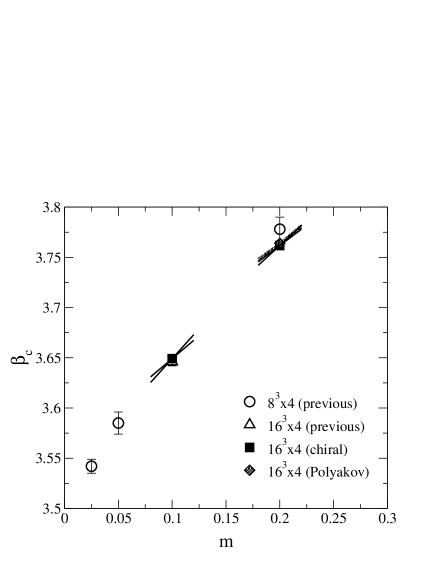
Figure 2: The transition “temperature”, $\beta_{c}$, as a function of $m$ in comparison with previous work[7]

6 Results for $\mu$ reweighting

We now turn to reweighting in chemical potential, $\mu$. As in [6], rather than applying the method to arbitrary parameter values, we trace out the transition point $\beta_{c}(\mu)$. Using Eq.(6), $<\overline{\psi}\psi>$ and the Polyakov Loop, $L$, are calculated as a function of $\mu$ together with their susceptibilities, $\chi_{\overline{\psi}\psi,L}$ (see Eq.(10)). In Figure 3, we plot $\chi_{\overline{\psi}\psi}$ against $\beta$ for various $\mu$. Note that the peak position moves as $\mu$ changes. The determination of the transition point $\beta_{c}$ from both the chiral condensate and the Polyakov loop (not shown here) are found to be in agreement.

Figure 3: The $\mu$ dependency of $\chi_{\overline{\psi}\psi}$ as a function of $\beta$ in the neighbourhood of $m=0.2$ for the chiral susceptibility.

Because we have calculated all quantities to $O(\mu^{2})$ we can extract $\beta_{c}$ and fit it to a quadratic in $\mu$. (In fact, it can be shown[4] that the first derivative ${\rm d}\beta_{c}/{\rm d}\mu=0$.) We find ${\rm d}^{2}\beta_{c}/{\rm d}\mu^{2}=1.1\pm 50\%$ for both quark masses $m=0.1$ and 0.2.

We now use

$$\frac{{\rm d}^{2}T_{c}}{{\rm d}\mu^{2}}=-\frac{1}{N_{t}^{2}T_{c}}\left.\frac{{\rm d}^{2}\beta_{c}}{{\rm d}\mu^{2}}\right/\left(a\frac{{\rm d}\beta}{{\rm d}a}\right),$$ (11)

to convert ${\rm d}^{2}\beta_{c}/{\rm d}\mu^{2}$ into physical units, with the beta-function ${\rm d}\beta/{\rm d}a$ coming from string tension data[7]. We find $T_{c}\frac{{\rm d}^{2}T_{c}}{{\rm d}\mu^{2}}\approx-0.14$ at $ma=0.1$.

Figure 4: The transition temperature, $T_{c}$, as a function of $\mu$. The diamond symbol is the endpoint of the first order transition obtained by Fodor and Katz[6]

Figure 4 shows the phase transition curve $T_{c}(\mu)$ obtained from this method. On this graph we have plotted the Fodor-Katz point[6] which is within our errors, confirming our method. Also shown is the $\mu$ value corresponding to RHIC. It is interesting to extrapolate the curve $T_{c}(\mu)$ to the horizontal axis (as shown). It is known that the transition (at $T\approx 0$) between ordinary hadronic matter and quark matter occurs at around $\mu\approx 400$ MeV. This is at a smaller value of $\mu$ than the horizontal intercept of our data indicating (not surprisingly) the presence of higher order terms in the Taylor expansion and/or a breakdown in our method at these large values of $\mu$.

This motivates the question: for what range in $\mu$ do we expect our method to be accurate (and converge to the correct answer)? We have studied this issue by calculating the complex phase, $\theta$, of the fermionic determinant (which enters in the reweighting factor in Eq.(5)), i.e.

$$\det M=|\det M|{\rm e}^{i\theta}$$ (12)

The reweighting method will fail when the fluctuations (standard deviation) in $\theta$ are larger than $O(\pi/2)$. Taylor expanding Eq.(12) and noting that only odd derivatives contribute to the complex phase $\theta$, we find that the standard deviation $\Delta\theta\sim O(\pi/2)$ at around $\mu/T_{c}\sim 0.5$. Since this is around five times the $\mu$ value of RHIC, we can confirm that our method is applicable for RHIC physics.

An interesting dynamical quark effect can be uncovered when studying the Polyakov Loop susceptibility, $\chi_{L}$. For $\mu<0$, anti-quarks are dynamically generated which screen colour charge. This leads to a reduction in the free energy of a single quark, and a corresponding reduction in the strength of the singularity at the transition. We observe this effect by noting that the peak height of $\chi_{L}$ is smaller for $\mu<0$ compared with $\mu>0$[4].

7 Pressure and energy density

Of great interest for heavy ion collision experiments is the study of the pressure, $p$, and energy density $\epsilon$ and their $\mu$ dependence. We can obtain estimates of $p$ by employing the integral method[9]:

$$p=\frac{T}{V}\ln Z.$$ (13)

The first derivative of $p$ w.r.t. $\mu$ is related to the quark number density,

$$n_{q}=\frac{T}{V}\frac{\partial\ln Z}{\partial\mu},$$ (14)

and the second derivative to the singlet quark number susceptibility, $\chi_{S}$. Both $n_{q}$ and $\chi_{S}$ can be calculated in terms of the quark matrix, $M$.

Using the above to estimate $p$ at the RHIC point we find that $p$ increases by around 1% from its $\mu=0$ value.

The energy density, $\epsilon$, can be obtained from

$$\frac{\epsilon-3p}{T^{4}}\approx-\frac{1}{VT^{3}}\frac{\partial\ln{Z}}{\partial\beta}\left(\frac{1}{a}\frac{\partial a}{\partial\beta}\right)^{-1}.$$ (15)

The derivatives of Eq.(15) can be expressed in terms of $n_{q}$ and $\chi_{S}$. Combining this with the above calculation of $p$, we obtain a value for $\epsilon$ alone. We find that, at the RHIC point, there is again only a 1% deviation from $\epsilon(\mu=0)$.

Finally we study the variation of $p$ and $\epsilon$ along the transition line $T_{c}(\mu)$. (The above calculations were performed at fixed $T$.) Our aim is to determine whether $p$ and $\epsilon$ are constant along $T_{c}(\mu)$. The constant $p$ line is defined as

$$\Delta p=\frac{\partial p}{\partial T}\Delta T+\frac{\partial p}{\partial(\mu^{2})}\Delta(\mu^{2})=0,$$ (16)

with a similar expression for the constant $\epsilon$ line. Using the above and the value determined earlier for the rate of change of $T_{c}$ with $\mu$, we find that the value of both $p$ and $\epsilon$ along the transition line $T_{c}(\mu)$ is consistent with zero with our current precision[4].

8 Conclusions

This work (which is published in full elsewhere[4]) has outlined a new method of determining thermal properties of QCD at non-zero chemical potential from the lattice. This approach is based on Taylor expanding the Ferrenberg-Swendsen reweighting scheme.

Using this method, the susceptibilities in the chiral condensate and Polyakov loop were determined and their peak positions used to define the transition point, $T_{c}$. As a warmup exercise, the reweighting technique was used to determine the transition point as a function of the quark mass, $m$ confirming earlier work. The method was then applied to obtaining $T_{c}$ as a function of chemical potential, $\mu$, confirming the work of Fodor and Katz[6]. Very recent work of de Forcrand and Philipsen, who studied the transition temperature for imaginary $\mu$ and then analytically continued these results to real-valued $\mu$ also confirm our results[10].

The region of applicability of our method was studied by calculating the fluctuations in the phase of the reweighting factor. This region was found to be substantial and easily covers the physically interesting values of $\mu$ appropriate for RHIC physics.

We also extracted information about the pressure, $p$, and energy density, $\epsilon$, as a function of chemical potential. We found that the variation in these quantities from their values at $\mu=0$ is tiny. This leads us to conclude that RHIC physics well approximated by $\mu=0$ physics. Furthermore we find that $p$ and $\epsilon$ are approximately constant along the transition line $T_{c}(\mu)$.

The success of this work motivates the use of lighter, more physical quark masses, and the study of (2+1) dynamical flavours to correctly model real world physics.

References

- [1] see http://www1.msfc.nasa.gov/NEWSROOM/news/releases/2002/02-082.html (NASA Press release); and J. Drake et al., The Astrophysical Journal, June 20 2002 to appear.
- [2] For a recent announcement from CERN, see http://cern.web.cern.ch/CERN/Announcements/2000/NewStateMatter/.
- [3] For a review, see S.J. Hands, Nucl.Phys. Proc.Suppl. 106 (2002) 142, hep-lat/0109034.
- [4] C.R. Allton, S. Ejiri, S.J. Hands, O. Kaczmarek, F. Karsch, E. Laermann, Ch. Schmidt, L. Scorzato, hep-lat/0204010.
- [5] A.M. Ferrenberg and R.H. Swendsen, Phys. Rev. Lett. 61 (1988) 2635; Phys. Rev. Lett. 63 (1989) 1195.
- [6] Z. Fodor and S.D. Katz, hep-lat/0104001; JHEP 0203:014,2002 hep-lat/0106002.
- [7] F. Karsch, E. Laermann, and A. Peikert, Phys. Lett. B478 (2000) 447; Nucl. Phys. B605 (2001) 579.
- [8] U.M. Heller, F. Karsch, and B. Sturm, Phys. Rev. D60 (1999) 114502.
- [9] J. Engels, J. Fingberg, F. Karsch, D. Miller and M. Weber, Phys. Lett. B252 (1990) 625.
- [10] Ph. de Forcrand and O. Philipsen, hep-lat/0205016.