IFT-02-18 UCD-02-09 DFF-389-06-02 June, 2002

ABSTRACT

The scalar sector of the Randall-Sundrum model is discussed. The effective potential for the Standard Model Higgs-boson ($h$) interacting with Kaluza-Klein excitations of the graviton ($h_{\mu}^{\nu\,n}$) and the radion ($\phi$) has been derived and it has been shown that only the Standard Model vacuum solution of $\partial V/\partial h=0$ is allowed. The theoretical and experimental consequences of the curvature-scalar mixing $\xi\,R\,\widehat{H}^{\dagger}\widehat{H}$ introduced on the visible brane are considered and simple sum rules that relate the couplings of the mass eigenstates $h$ and $\phi$ to pairs of vector bosons and fermions are derived. The sum rule for the $ZZh$ and $ZZ\phi$ couplings in combination with LEP/LEP2 data implies that not both the $h$ and $\phi$ can be light. We present explicit results for the still allowed region in the $(m_{h},m_{\phi})$ plane that remains after imposing the LEP upper limits for non-standard scalar couplings to a $ZZ$ pair. The phenomenological consequences of the mixing are investigated and, in particular, it is shown that the Higgs-boson decay $h\to\phi\phi$ would provide an experimental signature for non-zero $\xi$ and can have a very substantial impact on the Higgs-boson searches, having $BR(h\to\phi\phi)$ as large as $30\div 40\,\%$.

PACS: 04.50.+h, 12.60.Fr

Keywords: extra dimensions, Higgs-boson sector, Randall-Sundrum model

1 Introduction

Although the Standard Model (SM) of electroweak interactions describes successfully almost all existing experimental data the model suffers from many theoretical drawbacks. One of these is the hierarchy problem: namely, the SM can not consistently accommodate the weak energy scale ${\cal O}(1\;\hbox{TeV})$ and a much higher scale such as the Planck mass scale ${\cal O}(10^{19}\;\hbox{GeV})$. Therefore, it is commonly believed that the SM is only an effective theory emerging as the low-energy limit of some more fundamental high-scale theory that presumably could contain gravitational interactions. In the last few years there have been many models proposed that involve extra dimensions. These models have received tremendous attention since they could provide a solution to the hierarchy problem. One of the most attractive attempts has been formulated by Randall and Sundrum [1], who postulated a 5D universe with two 4D surfaces (“3-branes”). All the SM particles and forces with the exception of gravity are assumed to be confined to one of those 3-branes called the visible brane. Gravity lives on the visible brane, on the second brane (the “hidden brane”) and in the bulk. All mass scales in the 5D theory are of the order of the Planck mass. By placing the SM fields on the visible brane, all the mass terms (of the order of the Planck mass) are rescaled by an exponential suppression factor (the “warp factor”) $\Omega_{0}\equiv e^{-m_{0}b_{0}/2}$, which reduces them down to the weak scale ${\cal O}(1\;\hbox{TeV})$ on the visible brane without any severe fine tuning. To achieve the necessary suppression, one needs $m_{0}b_{0}/2\sim 35$. This is a great improvement compared to the original problem of accommodating both the weak and the Planck scale within a single theory.

In order to obtain a consistent solution to the Einstein equations corresponding to a low-energy effective theory that is flat, the branes must have equal but opposite cosmological constants and these must be precisely related to the bulk cosmological constant.

The model is defined by the 5D action:

$$S = -\int d^{4}x\,dy\sqrt{-\widehat{g}}\left({R\over 2\widehat{\kappa}^{2}}+\Lambda\right)$$

$$+\int d^{4}x\,\sqrt{-g_{hid}}({\cal L}_{hid}-V_{hid})+\int d^{4}x\,\sqrt{-g_{vis}}({\cal L}_{vis}-V_{vis}),$$

where $\widehat{g}^{\widehat{\mu}\widehat{\nu}}$ ($\widehat{\mu},\widehat{\nu}=0,1,2,3,4$) is the bulk metric and $g_{hid}^{\mu\nu}(x)\equiv\widehat{g}^{\mu\nu}(x,y=0)$ and $g_{vis}^{\mu\nu}(x)\equiv\widehat{g}^{\mu\nu}(x,y=1/2)$ ($\mu,\nu=0,1,2,3$) are the induced metrics on the branes. One finds that if the bulk and brane cosmological constants are related by $\Lambda/m_{0}=-V_{hid}=V_{vis}=-6m_{0}/\hat{\kappa}^{2}$ and if periodic boundary conditions identifying $(x,y)$ with $(x,-y)$ are imposed, then the 5D Einstein equations lead to the following metric:

$$ds^{2}=e^{-2\sigma(y)}\eta_{\mu\nu}dx^{\mu}dx^{\nu}-b_{0}^{2}dy^{2},$$ (2)

where $\sigma(y)=m_{0}b_{0}\left[y(2\theta(y)-1)-2(y-1/2)\theta(y-1/2)\right]$; $b_{0}$ is a constant parameter that is not determined by the action, Eq. (1). Gravitational fluctuations around the above background metric will be defined through the replacement:

$$\eta_{\mu\nu}\to\eta_{\mu\nu}+\epsilon h_{\mu\nu}(x,y)\;\;\;\;\;\;b_{0}\to b_{0}+b(x)\,.$$ (3)

Below we will be expanding in powers of $\epsilon h_{\mu\nu}=\sqrt{2}\hat{\kappa}h_{\mu\nu}$ and $b(x)/b_{0}$.

The paper is organized as follows. First, in Sec. 2 we derive the effective potential for the SM Higgs-boson sector interacting with Kaluza-Klein excitations of the graviton ($h_{\mu}^{\nu\,n}$) and the radion ($\phi$). In Sec. 3, we introduce the curvature-scalar mixing $\xi\,R\,\widehat{H}^{\dagger}\widehat{H}$ and discuss its consequences for couplings and interactions. In Sec. 4, we discuss some phenomenological aspects of the scalar sector, focusing on the particularly important possibility of $h\to\phi\phi$ decays. We summarize our results in Sec. 5.

Our work extends in several ways the already extensive literature [2, 3, 4, 5, 6, 7, 8, 9] on the phenomenology of the Randall-Sundrum model. We focus in particular on the case where the radion is substantially lighter than the Higgs boson and the important impacts of Higgs-radion mixing in this case.

2 The effective potential

The canonically normalized massless radion field $\phi_{0}(x)$ is defined by:

$$\phi_{0}(x)\equiv\left({6\over\widehat{\kappa}^{2}m_{0}}\right)^{1/2}\Omega_{b}(x)=\left({6\over\widehat{\kappa}^{2}m_{0}}\right)^{1/2}e^{-m_{0}b(x)/2}\,.$$ (4)

Keeping in mind that $h_{\mu\nu}(x,y)$ depends both on $x$ and $y$, we use the KK expansion in the extra dimension

$$h_{\mu\nu}(x,y)=\sum_{n}h_{\mu\nu}^{n}(x){\chi^{n}(y)\over\sqrt{b}_{0}}\,.$$ (5)

The total 4D effective potential (up to the terms of the order of ${\cal O}[(\epsilon h_{\mu\nu})^{3}]$) has been determined in Ref.[10]. Restricting ourselves to the trace part of $h_{\mu\nu}^{n}\sim{\textstyle{1\over 4}}\eta_{\mu\nu}\overline{h}^{n}$ the result is the following:

$$V_{eff}=V_{eff}^{brane}+V_{eff}^{KK}=$$

$$\left(1+{1\over\widehat{\Lambda}_{W}}\sum_{n}\overline{h}^{n}+{1\over 4\widehat{\Lambda}_{W}^{2}}\sum_{n}\sum_{m}\overline{h}^{n}\overline{h}^{m}+\cdots\right)\left[\left(1+{\phi_{0}\over\Lambda_{\phi}}\right)^{4}V(h_{0})+{\textstyle{1\over 2}}m_{\phi_{0}}^{2}\phi_{0}^{2}\right]$$

$$-{3\over 16}\sum_{n}m_{n}^{2}(\overline{h}^{n})^{2}+\cdots\,,$$ (6)

where $m_{n}$ is the KK-graviton mass, $\widehat{\Lambda}_{W}\equiv 2\sqrt{b_{0}}/[\epsilon\chi^{n}(1/2)]\simeq\sqrt{2}M_{Pl}\Omega_{0}$ and we have expanded around the vacuum expectation values for the radion, $\phi_{0}\to\langle\phi_{0}\rangle+\phi_{0}\equiv\Lambda_{\phi}+\phi_{0}$. In order to stabilize the size of the extra dimension we have introduced the radion mass $m_{\phi_{0}}$ without specifying its origin. Restricting ourself to the perturbative regime we will look for the minimum of $V_{eff}$ that satisfies $\sum_{n}\overline{h}^{n}/\widehat{\Lambda}_{W}\ll 1$ and $b(x)/b_{0}\ll 1$, the latter being equivalent to $\phi_{0}(x)/\Lambda_{\phi}\ll 1$:

$$\left({1\over\widehat{\Lambda}_{W}}+\frac{1}{2\widehat{\Lambda}_{W}^{2}}\sum_{n}\overline{h}^{n}\right)\left[\left(1+{\phi_{0}\over\Lambda_{\phi}}\right)^{4}V+\frac{1}{2}m_{\phi}^{2}\phi_{0}^{2}\right]-{3\over 8}m_{n}^{2}\overline{h}^{n} = 0$$

(7)

$$\left(1+{1\over\widehat{\Lambda}_{W}}\sum_{n}\overline{h}^{n}+{1\over 4\widehat{\Lambda}_{W}^{2}}\sum_{n}\sum_{m}\overline{h}^{n}\overline{h}^{m}\right)4\left(1+{\phi_{0}\over\Lambda_{\phi}}\right)^{3}{V\over\Lambda_{\phi}}+m_{\phi_{0}}^{2}\phi_{0} = 0$$

$$\left(1+{1\over\widehat{\Lambda}_{W}}\sum_{n}\overline{h}^{n}+{1\over 4\widehat{\Lambda}_{W}^{2}}\sum_{n}\sum_{m}\overline{h}^{n}\overline{h}^{m}\right)\left(1+{\phi_{0}\over\Lambda_{\phi}}\right)^{4}{\partial V(h_{0})\over\partial h_{0}} = 0\,.$$

There is only one solution of Eq. (LABEL:min3) consistent with $\phi_{0}/\Lambda_{\phi}\ll 1$ and $\overline{h}^{n}/\widehat{\Lambda}_{W}\ll 1$: namely, ${\partial V(h_{0})\over\partial h_{0}}=0$. For consistency of the RS model we must also require that $V(\langle h_{0}\rangle)=0$. If $V(\langle h_{0}\rangle)\neq 0$, then the visible brane tension would be shifted away from the very finely tuned RS solution to the Einstein equations. With these two ingredients, Eq. (LABEL:min2) implies that $\langle\phi_{0}\rangle=0$ at the minimum, implying that we have chosen the correct expansion point for $\phi_{0}$, and Eq. (7) then implies that $\langle\overline{h}^{n}\rangle=0$, i.e. we have expanded about the correct point in the $\overline{h}^{n}$ fields. However, it is only if $m_{\phi_{0}}^{2}>0$ that $\langle\phi_{0}\rangle=0$ is required by the minimization conditions. If $m_{\phi_{0}}=0$, then Eq. (7) still requires $\langle\overline{h}^{n}\rangle=0$ but all equations are satisfied for any $\langle\phi_{0}\rangle$.

Finally, we note that since $\partial V/\partial h_{0}=0$ at the minimum (even after including interactions with the radion and KK gravitons) there are no terms in the potential that are linear in the Higgs field $h_{0}$ (so in particular no $h_{0}-\phi_{0}$ mass mixing emerge). We will return to this observation in the next section of the paper.

3 The curvature-scalar mixing

Having determined the vacuum structure of the model, we are in a position to discuss the possibility of mixing between gravity and the electroweak sector. The simplest example of the mixing is described by the following action [11]:

$$S_{\xi}=\xi\int d^{4}x\sqrt{g_{\rm vis}}R(g_{\rm vis})\widehat{H}^{\dagger}\widehat{H}\,,$$ (10)

where $R(g_{\rm vis})$ is the Ricci scalar for the metric induced on the visible brane $g^{\mu\nu}_{\rm vis}=\Omega_{b}^{2}(x)(\eta^{\mu\nu}+\epsilon h^{\mu\nu})$. Using $H_{0}=\Omega_{0}\widehat{H}$ one obtains [12]

$$\xi\sqrt{g_{\rm vis}}R(g_{\rm vis})\widehat{H}^{\dagger}\widehat{H}=6\xi\Omega(x)\left(-\Box\Omega(x)+\epsilon h_{\mu\nu}\partial^{\mu}\partial^{\nu}\Omega+\cdots\right)H_{0}^{\dagger}H_{0}\,.$$ (11)

To isolate the kinetic energy terms we use the expansion

$$H_{0}={1\over\sqrt{2}}(v_{0}+h_{0})\,,\quad\Omega(x)=1+{\phi_{0}\over\Lambda_{\phi}}\,.$$ (12)

The $h_{\mu\nu}$ term of Eq. (11) does not contribute to the kinetic energy since a partial integration would lead to $h_{\mu\nu}\partial^{\mu}\partial^{\nu}\Omega=-\partial^{\mu}h_{\mu\nu}\partial^{\nu}\Omega=0$ by virtue of the gauge choice, $\partial^{\mu}h_{\mu\nu}=0$. We thus find the following kinetic energy terms:

$${\cal L}=-{\textstyle{1\over 2}}\left\{1+6\gamma^{2}\xi\right\}\phi_{0}\Box\phi_{0}-{\textstyle{1\over 2}}\phi_{0}m_{\phi_{0}}^{2}\phi_{0}-{\textstyle{1\over 2}}h_{0}(\Box+m_{h_{0}}^{2})h_{0}-6\gamma\xi\phi_{0}\Box h_{0}\,,$$ (13)

where $\gamma\equiv v_{0}/\Lambda_{\phi}$ and $m_{h_{0}}^{2}=2\lambda v^{2}$ and $m_{\phi_{0}}^{2}$ are the Higgs and radion masses before the mixing. The above differs from Ref. [13] by the extra $\phi_{0}\Box\phi_{0}$ piece proportional to $\xi$.

We define the mixing angle $\theta$ by

$$\tan 2\theta\equiv 12\gamma\xi Z{m_{h_{0}}^{2}\over m_{\phi_{0}}^{2}-m_{h_{0}}^{2}(Z^{2}-36\xi^{2}\gamma^{2})}\,,$$ (14)

where

$$Z^{2}\equiv 1+6\xi\gamma^{2}(1-6\xi)\,.$$ (15)

In terms of these quantities, the states that diagonalize the kinetic energy and have canonical normalization are $h$ and $\phi$ with:

$$h_{0} = \left(\cos\theta-{6\xi\gamma\over Z}\sin\theta\right)h+\left(\sin\theta+{6\xi\gamma\over Z}\cos\theta\right)\phi\equiv dh+c\phi$$ (16)

$$\phi_{0} = -\cos\theta{\phi\over Z}+\sin\theta{h\over Z}\equiv a\phi+bh\,.$$ (17)

(Our sign convention for $\phi_{0}$ is opposite to that chosen for $r$ in Ref. [12].) To maintain positive definite kinetic energy terms for the $h$ and $\phi$, we must have $Z^{2}>0$. (Note that this implies that $\beta\equiv 1+6\xi\gamma^{2}>0$ is implicitly required.) The corresponding mass-squared eigenvalues are

$$m_{\pm}^{2}={1\over 2Z^{2}}\left(m_{\phi_{0}}^{2}+\beta m_{h_{0}}^{2}\pm\left\{[m_{\phi_{0}}^{2}+\beta m_{h_{0}}^{2}]^{2}-4Z^{2}m_{\phi_{0}}^{2}m_{h_{0}}^{2}\right\}^{1/2}\right)\,.$$ (18)

It follows from the above formula that $m_{\pm}$ cannot be too close to being degenerate in mass, depending on the precise values of $\xi$ and $\gamma$, see Ref.[10].

We now turn to the important interactions of the $h$, $\phi$ and $h_{\mu\nu}^{n}$. We begin with the $ZZ$ couplings of the $h$ and $\phi$. The $h_{0}$ has standard $ZZ$ coupling while the $\phi_{0}$ has $ZZ$ coupling deriving from the interaction $-{\phi_{0}\over\Lambda_{\phi}}T_{\mu}^{\mu}$ using the covariant derivative portions of $T_{\mu}^{\mu}(h_{0})$. The result for the $\eta_{\mu\nu}$ portion of the $ZZ$ couplings is:

$$g_{ZZh}=\frac{g\,m_{Z}}{c_{W}}\left(d+\gamma b\right),\;\;\;\;\;\;g_{ZZ\phi}=\frac{g\,m_{Z}}{c_{W}}\left(c+\gamma a\right)\,,$$ (19)

where $a$, $b$, $c$ and $d$ are defined through Eqs. (16,17) and $g$, $c_{W}$ denote the $SU(2)$ gauge coupling and cosine of the Weinberg angle, respectively . The $WW$ couplings are obtained by replacing $gm_{Z}/c_{W}$ by $gm_{W}$. Notice also an absence of $Zh\phi$ tree level couplings. Next, we consider the fermionic couplings of the $h$ and $\phi$. The $h_{0}$ has standard fermionic couplings and the fermionic couplings of the $\phi_{0}$ derive from $-{\phi_{0}\over\Lambda_{\phi}}T_{\mu}^{\mu}$ using the Yukawa interaction contributions to $T_{\mu}^{\mu}$. One obtains results in close analogy to the $VV$ couplings just considered:

$$g_{f\bar{f}h}=-\frac{g\,m_{f}}{2\,m_{W}}(d+\gamma b)\;\;\;\;\;\;g_{f\bar{f}\phi}=-\frac{g\,m_{f}}{2\,m_{W}}(c+\gamma a)$$ (20)

For small values of $\gamma$, the $g_{ZZh}$ and $g_{ZZ\phi}$ have the expansions:

$$g_{ZZh} = \left(\frac{g\,m_{Z}}{c_{W}}\right)\left[1+{\cal O}(\gamma^{2})\right],$$ (21)

$$g_{ZZ\phi} = \left(\frac{g\,m_{Z}}{c_{W}}\right)\left[-\gamma\left(1+\frac{6\xi m_{\phi}^{2}}{m_{h}^{2}-m_{\phi}^{2}}\right)+{\cal O}(\gamma^{3})\right]$$

Entirely analogous results apply for the fermionic couplings.

The following simple and exact sum rules (independently noted in [6]) follow from the definitions of $a,b,c,d$:

$${g_{ZZh}^{2}+g_{ZZ\phi}^{2}\over\left(\frac{g\,m_{Z}}{c_{W}}\right)^{2}}={g_{f\overline{f}h}^{2}+g_{f\overline{f}\phi}^{2}\over\left(\frac{gm_{f}}{2m_{W}}\right)^{2}}=\left[1+{\gamma^{2}(1-6\xi)^{2}\over Z^{2}}\right]\equiv R^{2}\,.$$ (22)

Note that $R^{2}>1$ is a result of the non-orthogonality of the relations Eq. (16) and Eq. (17). Of course, $R^{2}=1$ in the conformal limit, $\xi=1/6$. It is important to note that $Z\to 0$ would lead to divergent $ZZ$ and $f\overline{f}$ couplings for the $\phi$. As noted earlier, this was to be anticipated since $Z\to 0$ corresponds to vanishing of the radion kinetic term before going to canonical normalization. After the rescaling that guarantees the canonical normalization, if $Z\to 0$ the radion coupling constants blow up: $g_{ZZ\phi}\propto(c+\gamma a)\simeq 1/(6\xi\gamma Z)+{\cal O}(Z)$. To have $Z^{2}>0$, $\xi$ must lie in the region:

$$\frac{1}{12}\left(1-\sqrt{1+\frac{4}{\gamma^{2}}}\right)\leq\xi\leq\frac{1}{12}\left(1+\sqrt{1+\frac{4}{\gamma^{2}}}\right)\,.$$ (23)

As an example, for $\Lambda_{\phi}=5\;\hbox{TeV}$, $Z^{2}>0$ corresponds to the range $-3.31\leq\xi\leq 3.47$. Of course, if we choose $\xi$ sufficiently close to the limits, $Z^{2}\to 0$ implies that the couplings, as characterized by $R^{2}$ will become very large. Thus, we should impose bounds on $\xi$ that keep $R^{2}$ moderate in size. For example, for $\Lambda_{\phi}=5\;\hbox{TeV}$, $R^{2}$ in Eq. (22) takes the values 2.48 and 1.96 at $\xi=-2.5$ and $\xi=2.5$, respectively. Therefore we will impose an overall restriction of $R\leq 5$. In practice, this bound seldom plays a role, being almost always superseded by the constraint limiting $\xi$ according to the degree of $m_{h}-m_{\phi}$ degeneracy.

The final crucial ingredient for the phenomenology that we shall consider is the tri-linear interactions among the $h$ and $\phi$ and $h_{\mu\nu}^{n}$ fields. In particular, these are crucial for the decays of these three types of particles. The tri-linear interactions derive from four basic sources.

1. First, we have the cubic interactions coming from

   $${\cal L}\ni-V(H_{0})=-\lambda(H_{0}^{\dagger}H_{0}-\frac{1}{2}v_{0}^{2})^{2}=-\lambda(v_{0}^{2}h_{0}^{2}+v_{0}h_{0}^{3}+\frac{1}{4}h_{0}^{4})\,,$$ (24)

   after substituting $H_{0}=\frac{1}{\sqrt{2}}(v_{0}+h_{0})$. Since $\lambda$ is related to the bare Higgs-boson mass in a usual way: $m_{h_{0}}^{2}=2\lambda v_{0}^{2}$ the $h_{0}^{3}$ interaction can be expressed as

   $${\cal L}\ni-{m_{h_{0}}^{2}\over 2v_{0}}h_{0}^{3}\,.$$ (25)

2. Second, there is the interaction of the radion $\phi_{0}$ with the stress-energy momentum tensor trace:

   $${\cal L}\ni-{\phi_{0}\over\Lambda_{\phi}}T_{\mu}^{\mu}(h_{0})=-{\phi_{0}\over\Lambda_{\phi}}\left(-\partial^{\rho}h_{0}\partial_{\rho}h_{0}+4\lambda v_{0}^{2}h_{0}^{2}\right)\,.$$ (26)

3. Thirdly, we have the interaction of the KK-gravitons with the contribution to the stress-energy momentum tensor coming from the $h_{0}$ field:

   $${\cal L}\ni-{\epsilon\over 2}h_{\mu\nu}T^{\mu\nu}\ni-{1\over\widehat{\Lambda}_{W}}\sum_{n}h_{\mu\nu}^{n}\partial^{\mu}h_{0}\partial^{\nu}h_{0}\,,$$ (27)

   where we have kept only the derivative contributions and we have dropped (using the gauge $h_{\mu}^{\mu\,n}=0$) the $\eta^{\mu\nu}$ parts of $T^{\mu\nu}$.

4. Finally, we have the $\xi$-dependent tri-linear components of Eq. (11):

   $$6\xi\Omega(x)\left(-\Box\Omega(x)+\epsilon h_{\mu\nu}\partial^{\mu}\partial^{\nu}\Omega(x)\right)H_{0}^{\dagger}H_{0}\ni\Bigl{[}-3\frac{\xi}{\Lambda_{\phi}}h_{0}^{2}\Box\phi_{0}$$

   $$-6\xi\frac{v_{0}}{\Lambda_{\phi}^{2}}h_{0}\phi_{0}\Box\phi_{0}-12\xi\frac{v_{0}}{\widehat{\Lambda}_{W}\Lambda_{\phi}}\sum_{n}h_{\mu\nu}^{n}\partial^{\mu}\phi_{0}\partial^{\nu}h_{0}$$

   $$-6\xi\frac{v_{0}^{2}}{\widehat{\Lambda}_{W}\Lambda_{\phi}^{2}}\sum_{n}h_{\mu\nu}^{n}\partial^{\mu}\phi_{0}\partial^{\nu}\phi_{0}\Bigr{]}$$ (28)

   where we have employed $\partial^{\mu}h_{\mu\nu}^{n}=0$, used the traceless gauge condition $h_{\mu}^{\mu\,n}=0$, and also used the symmetry of $h_{\mu\nu}$.

As seen from the above list, without the curvature-Higgs mixing the lagrangian does not contain any interactions linear in the Higgs field, therefore vertices like $\phi^{2}h$ and $h^{n}\phi h$ (that follows from Eq. (28)) are a clear indication for the curvature-Higgs mixing. As we shall see, the $\phi^{2}h$ coupling could also be of considerable phenomenological importance leading to $h\to\phi\phi$ decays. The $h^{n}\phi h$ coupling would be relevant for $h\to\phi h^{n}$, however for the parameters range considered here that decay would be relatively rare.

4 Phenomenology

We begin by discussing the restrictions on the $h,\phi$ sector imposed by LEP Higgs-boson searches. Since no scalar boson (s) was observed in the process $e^{+}e^{-}\to Zs$, LEP/LEP2 provides an upper limit for the coupling of a $ZZ$ pair to the scalar as a function of the scalar mass. Here we will employ the limits from [14, 15, 16].

The first question that arises is whether both the $\phi$ and the $h$ could be light without either having been detected at LEP and LEP2. The sum rule of Eq. (22) implies that this is impossible since the couplings of the $h$ and $\phi$ to $ZZ$ cannot both be suppressed. For any given value of $m_{h}$ and $m_{\phi}$, the range of $\xi$ is limited by: (a) the constraint limiting $\xi$ according to the degree of $m_{h}-m_{\phi}$ degeneracy; (b) the constraint that $Z^{2}>0$, Eq. (15); and (c) the requirements that $g_{ZZh}^{2}$ and $g_{ZZ\phi}^{2}$ both lie below any relevant LEP/LEP2 limit. The regions in the $(\xi,m_{\phi})$ plane consistent with the first two constraints as well as with $R<5$ are shown in Figs. 2 and 2 for $m_{h}=112\;\hbox{GeV}$ and $m_{h}=120\;\hbox{GeV}$, respectively, assuming a value of $\Lambda_{\phi}=5\;\hbox{TeV}$. For the most part, it is the degeneracy constraint (a) that defines the theoretically acceptable regions shown. The regions within the theoretically acceptable regions that are excluded by the LEP/LEP2 limits are shown by the yellow shaded regions, while the allowed regions are in blue. For $m_{h}=112\;\hbox{GeV}$, the LEP/LEP2 limits exclude a large portion of the theoretically consistent parameter space. For $m_{h}=110\;\hbox{GeV}$ (not plotted), the sum rule of Eq. (22) results in all of the theoretically allowed parameter space being excluded by LEP/LEP2 constraints. For $m_{h}=120\;\hbox{GeV}$, the LEP/LEP2 limits do not apply to the $h$ and it is only for $m_{\phi}\mathrel{\raise 1.29167pt\hbox{$<$\kern-7.5pt\lower 4.30554pt\hbox{$\sim$}}}115\;\hbox{GeV}$ and significant $g_{ZZ\phi}^{2}$ (requiring large $|\xi|$) that some points are ruled out by the LEP/LEP2 constraints. As a result, the allowed region is dramatically larger than for $m_{h}=112\;\hbox{GeV}$. The precise regions shown are somewhat sensitive to the $\Lambda_{\phi}$ choice, but the overall picture is always similar to that presented here for $\Lambda_{\phi}=5\;\hbox{TeV}$.

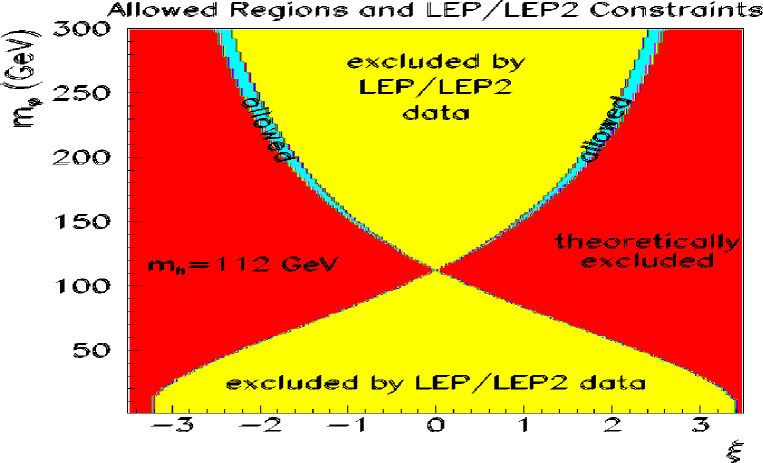
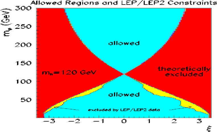
Figure 1: Allowed regions (see text) in $(\xi,m_{\phi})$ parameter space for $\Lambda_{\phi}=5\;\hbox{TeV}$ and $m_{h}=112\;\hbox{GeV}$. The dark red portion of parameter space is theoretically disallowed. The light yellow portion is eliminated by LEP/LEP2 constraints on the $ZZs$ coupling-squared $g_{ZZs}^{2}$ or on $g_{ZZs}^{2}BR(s\to b\overline{b})$, with $s=h$ or $s=\phi$.

Figure 2: As in Fig. 2 but for $m_{h}=120\;\hbox{GeV}$.

In order to illustrate LHC Higgs-boson discovery potential in the presence of the curvature-mixing we plot in Fig. 3 the ratio of the rates for $gg\to h\to\gamma\gamma$, $WW\to h\to\tau^{+}\tau^{-}$ and $gg\to t\overline{t}h\to t\overline{t}b\overline{b}$ (the latter two ratios being equal) to the corresponding rates for the SM Higgs boson. All the curves are plotted for the parameter range that is consistent with the theoretical and experimental constraints mentioned above. For this figure, we take $m_{h}=120\;\hbox{GeV}$ and $\Lambda_{\phi}=5\;\hbox{TeV}$ and show results for $m_{\phi}=20$, $55$ and $200\;\hbox{GeV}$. As will be discussed later, in the case of $m_{\phi}=55\;\hbox{GeV}$, the $h\to\phi\phi$ decay is substantial for large $|\xi|$. The resulting suppression of the standard LHC modes at the largest allowed $|\xi|$ values is most evident in the $W^{+}W^{-}\to h\to\tau^{+}\tau^{-}$ curves. Another important impact of mixing is through communication of the anomalous $gg$ coupling of the $\phi_{0}$ to the $h$ mass eigenstate. The result is that prospects for $h$ discovery in the $gg\to h\to\gamma\gamma$ mode could be either substantially poorer or substantially better than for a SM Higgs boson of the same mass, depending on $\xi$ and $m_{\phi}$.

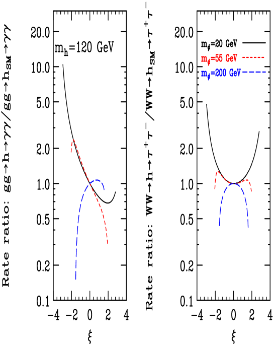
Figure 3: The ratio of the rates for $gg\to h\to\gamma\gamma$ and $WW\to h\to\tau^{+}\tau^{-}$ (the latter is the same as that for $gg\to t\overline{t}h\to t\overline{t}b\overline{b}$) to the corresponding rates for the SM Higgs boson. Results are shown for $m_{h}=120\;\hbox{GeV}$ and $\Lambda_{\phi}=5\;\hbox{TeV}$ as functions of $\xi$ for $m_{\phi}=20$, $55$ and $200\;\hbox{GeV}$.

At the LC, the potential for $h$ discovery is primarily determined by $g_{ZZh}^{2}$. As we have shown in Ref. [10], this coupling-squared (relative to the SM value) is often $>1$ (and can be as large as $\sim 5$), but can also fall to values as low as $\sim 0.4$, implying significant suppression relative to SM expectations. However the latter suppression is still well within the reach of the $e^{+}e^{-}\to Zh$ recoil mass discovery technique at a LC with $\sqrt{s}=500\;\hbox{GeV}$ and $L=500~{}\mbox{fb${}^{-1}$}$.

A particularly important feature of Figs. 2 and 2 is that once $m_{h}$ is large enough (typically $m_{h}\mathrel{\raise 1.29167pt\hbox{$>$\kern-7.5pt\lower 4.30554pt\hbox{$\sim$}}}115\;\hbox{GeV}$ is sufficient) it will generally be possible to find $\xi$ values for which a range of moderately small, and possibly even very small, $m_{\phi}$ values cannot be excluded by LEP/LEP2 constraints. In particular, $m_{\phi}<m_{h}/2$ (so that $h\to\phi\phi$ decays are possible) is typically not excluded for a substantial range of $\xi$. (The reverse is also true; allowed parameter regions exist for which $\phi\to hh$ decays are possible once $m_{\phi}\mathrel{\raise 1.29167pt\hbox{$>$\kern-7.5pt\lower 4.30554pt\hbox{$\sim$}}}100\;\hbox{GeV}$. However, for this paper we have chosen to focus on cases in which the $\phi$ is not very heavy.) With this in mind, we now turn to a discussion of branching ratios, focusing on the $h\to\phi\phi$ final mode:

$$\Gamma(h\to\phi\phi)={g_{\phi\phi h}^{2}\over 32\pi m_{h}\Lambda_{\phi}^{2}}(1-4r_{\phi})^{1/2}\,,$$ (29)

where $\lambda(1,r_{1},r_{2})\equiv 1+r_{1}^{2}+r_{2}^{2}-2r_{1}-2r_{2}-2r_{1}r_{2}$, $r_{\phi}=m_{\phi}^{2}/m_{h}^{2}$, $r_{n}=m_{n}^{2}/m_{h}^{2}$ and

$$g_{\phi\phi h}\equiv 2m_{\phi}^{2}\left[6a\xi(\gamma(ad+bc)+cd)+bc^{2}\right]$$ (30)

$$+m_{h}^{2}\;c\left[12ab\gamma\xi+2ad+bc(6\xi-1)\right]-4c(2ad+bc)m_{h_{0}}^{2}-3\gamma^{-1}c^{2}dm_{h_{0}}^{2}\,.$$

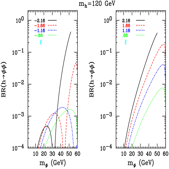
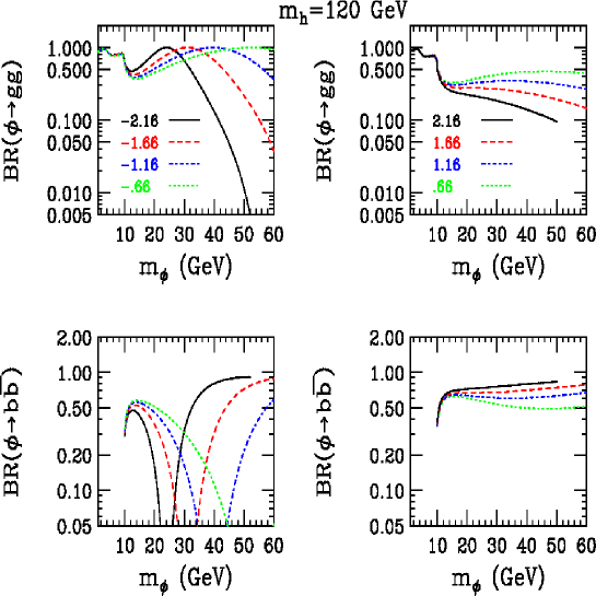
Figure 4: The branching ratios for $h\to\phi\phi$, $\phi\to gg$ and $\phi\to b\overline{b}$ for $m_{h}=120\;\hbox{GeV}$ and $\Lambda_{\phi}=5\;\hbox{TeV}$ as a function of $m_{\phi}$ for $\xi=-2.16$, $-1.66$, $-1.16$ and $-0.66$ (left-hand graphs) and for $\xi=0.66$, $1.16$, $1.66$, and $2.16$ (right-hand graphs).

The branching ratios for $h\to\phi\phi$ in the case of $m_{h}=120\;\hbox{GeV}$ and $\Lambda_{\phi}=5\;\hbox{TeV}$ are shown in Fig. 4 for various $\xi$ choices within the allowed region. The plots show that $h\to\phi\phi$ decays can be quite important at the largest $|\xi|$ values when $m_{\phi}$ is close to $m_{h}/2$. Detection of the $h\to\phi\phi$ decay mode could easily provide the most striking evidence for the presence of $\xi\neq 0$ mixing. In order to understand how to search for the $h\to\phi\phi$ decay mode, it is useful to know how the $\phi$ decays. In Fig. 4 we give detailed results for $BR(\phi\to gg)$ and $BR(\phi\to b\overline{b})$ for the same $m_{\phi}$ and $\xi$ values for which $BR(h\to\phi\phi)$ is plotted. (The $c\overline{c}$ and $\tau^{+}\tau^{-}$ channels supply the remainder.) For $\xi>0$, $BR(\phi\to b\overline{b})$ is always substantial and might make detection of the $h\to\phi\phi\to 4b$ and $h\to\phi\phi\to 2g2b$ final states possible. The $\phi\to\gamma\gamma$ decay mode always has a very tiny branching ratio and the related detection channels would not be useful.

One will probably first search for the $h$ in the modes that have been shown to be viable for the SM Higgs boson. We have given in Fig. 3 the rates for important LHC discovery modes relative to the corresponding SM values in the case of $m_{\phi}=55\;\hbox{GeV}$. Results for other $m_{\phi}<m_{h}/2$ values are similar in nature. We observe that the $WW\to h\to\tau^{+}\tau^{-}$ and $gg\to t\overline{t}h\to t\overline{t}b\overline{b}$ detection modes are generally sufficiently mildly suppressed that detection of the $h$ in these modes should be possible (assuming full $L=300~{}\mbox{fb${}^{-1}$}$ luminosity per detector). The $gg\to h\to\gamma\gamma$ detection mode could either be enhanced or significantly suppressed relative to the SM expectation. Once the $h$ has been detected in one of the SM modes, a dedicated search for the $h\to\phi\phi\to b\overline{b}b\overline{b}$ and $h\to\phi\phi\to b\overline{b}gg$ decay modes will be important. At the LHC, backgrounds for these modes will be substantial and a thorough Monte Carlo assessment will be needed.

5 Summary and Conclusions

We have discussed the scalar sector of the Randall-Sundrum model. The effective potential (defined as a set of interaction terms that contain no derivatives) for the Standard Model Higgs-boson sector interacting with Kaluza-Klein excitations of the graviton ($h_{\mu}^{\mu\,n}$) field and the radion ($\phi$) field has been derived. Without specifying its origin, a stabilizing mass-term for the radion has been introduced. After including this term, we have shown that only the Standard Model vacuum determined by $\partial V/\partial h=0$ is allowed. An important requisite property for the correct vacuum solution is that the effective potential does not contain any terms linear in the Higgs field.

Having confirmed that the usually assumed vacuum properties are correct, we pursue in more detail the phenomenology of the RS scalar sector, focusing in particular on results found in the presence of a curvature-scalar mixing $\xi\,R\,\widehat{H}^{\dagger}\widehat{H}$ contribution to the Lagrangian. Simple sum rules that relate Higgs-boson and radion couplings to pairs of vector bosons and fermions have been derived. Of particular interest is the fact that non-zero $\xi$ induces interactions linear in the Higgs field: $\phi^{2}h$ and $h^{n}h\phi$.

We derive the regions of parameter space that are excluded by direct LEP/LEP2 limits on scalar particles with $ZZ$ coupling as function of scalar mass. Of particular note is the fact that the sum rule for $ZZh$ and $ZZ\phi$ squared-couplings noted above implies that it is impossible for both the $h$ and $\phi$ to be light. However, even very light $\phi$ ($m_{\phi}<10\;\hbox{GeV}$) remains a possibility if $m_{h}\mathrel{\raise 1.29167pt\hbox{$>$\kern-7.5pt\lower 4.30554pt\hbox{$\sim$}}}115\;\hbox{GeV}$ and the (dominant) $\phi\to gg$ decays result in final states to which existing searches for on-shell $Z\to Z^{*}\phi$ decays would not have been very sensitive.

One particularly interesting complication for $\xi\neq 0$ is the presence of the non-standard decay channels, $h\to\phi\phi$ and $h\to h^{n}\phi$. These could easily be present since in the context of the RS model there is a possibility (perhaps even a slight preference) for the $\phi$ to be substantially lighter than the $h$. In particular, $m_{\phi}<m_{h}/2$ is a distinct possibility. We study in detail the phenomenology when $m_{\phi}\leq 60\;\hbox{GeV}$ for $m_{h}=120\;\hbox{GeV}$, so that the $h\to\phi\phi$ mode is present. Even for a relatively conservative choice of the new-physics scale, $\Lambda_{\phi}=5\;\hbox{TeV}$, this mode will be present at an observable level, and, at the largest $|\xi|$ values and for $m_{\phi}$ not far below $m_{h}/2$, can even substantially dilute the rates for the usual $h$ search channels. In any case, detection of $h\to\phi\phi$ is very important as it would provide a crucial experimental signature for non-zero $\xi$. For the less conservative choice of $\Lambda_{\phi}=1\;\hbox{TeV}$ and for a light $h$, e.g. $m_{h}=120\;\hbox{GeV}$, $BR(h\to\phi\phi)$ could easily be as large as $50\,\%$ for most of the theoretically allowed values of $m_{\phi}$ (which are near $m_{h}/2$) when $|\xi|$ is near the largest value allowed by theoretical and existing experimental constraints.

ACKNOWLEDGMENTS

The authors are grateful to the organizers of the Fifth European Meeting From the Planck Scale to the Electroweak Scale, “Supersymmetry and Brane Worlds” for creating a very warm and inspiring atmosphere during the meeting. B.G. thanks Z. Lalak, K. Meissner and J. Pawelczyk for useful discussions. J.F.G would like to thank J. Wells for useful discussions. B.G. is supported in part by the State Committee for Scientific Research under grant 5 P03B 121 20 (Poland). J.F.G. is supported by the U.S. Department of Energy and by the Davis Institute for High Energy Physics.

References

[1]
L. Randall, R. Sundrum,
Phys. Rev. Lett.83 (1999), 3370, hep-ph/9905221;
L. Randall, R. Sundrum,
Phys. Rev. Lett.83 (1999), 4690, hep-th/9906064.
[2]
S. B. Bae, P. Ko, H. S. Lee and J. Lee,
Phys. Lett. B 487, 299 (2000), hep-ph/0002224.
[3]
H. Davoudiasl, J. L. Hewett and T. G. Rizzo,
Phys. Rev. Lett. 84, 2080 (2000), hep-ph/9909255.
[4]
K. Cheung,
Phys. Rev. D 63, 056007 (2001), hep-ph/0009232.
[5]
H. Davoudiasl, J. L. Hewett and T. G. Rizzo,
Phys. Rev. D 63, 075004 (2001), hep-ph/0006041.
[6]
T. Han, G. D. Kribs and B. McElrath,
Phys. Rev. D 64, 076003 (2001), hep-ph/0104074.
[7]
S. C. Park, H. S. Song and J. Song,
Phys. Rev. D 63, 077701 (2001), hep-ph/0009245.
[8]
M. Chaichian, A. Datta, K. Huitu and Z. h. Yu,
Phys. Lett. B 524, 161 (2002), hep-ph/0110035.
[9]
J. L. Hewett and T. G. Rizzo,
hep-ph/0202155.
[10]
D. Dominici, B. Grzadkowski, J. F. Gunion, and M. Toharia, hep-ph/0206192.
[11]
J.J. van der Bij,
Acta Phys.Polon.B25 (1994), 827;
R. Raczka, M. Pawlowski,
Found.Phys.24 (1994), 1305, hep-th/9407137.