The Equation of State for Dense QCD and Quark Stars

Abstract

We calculate the equation of state for degenerate quark matter to leading order in hard-dense-loop (HDL) perturbation theory. We solve the Tolman-Oppenheimer-Volkov equations to obtain the mass-radius relation for dense quark stars. Both the perturbative QCD and the HDL equations of state have a large variation with respect to the renormalization scale for $\mu\,\raisebox{-2.84544pt}{$\stackrel{{\scriptstyle<}}{{\sim}}$}$ 1 GeV which leads to large theoretical uncertainties in the quark star mass-radius relation.

I Introduction

An understanding of the behavior of quantum chromodynamics (QCD) at high density is crucial to describing the physics of compact stars. This is due to the fact that the nuclear matter within these compact objects may be sufficiently dense to undergo a phase transition to a deconfined or “quark-matter” phase. Of particular interest is the possibility that stars which have a significant quark-matter component could have a dramatically different mass-radius relationship than normal neutron stars [1]. However, in order to make definitive statements about the mass-radius relationship for such objects one needs a reliable calculation of the equation of state of high-density QCD.

In recent years high-density QCD has received considerable attention due to the possible breaking of color gauge symmetry which gives rise to color superconductivity. As a consequence of this, QCD has a very complicated phase diagram which depends on the number and masses of the dynamical quarks [2]. It would therefore seem that the effect of the superconducting phase on the equation of state would need to be taken into account; however, despite the fact that the gaps for color superconductivity are inherently non-perturbative, their effect on the equation of state for high-density QCD is expected to be small [3]. Therefore, it is possible to use equations of state that have been derived neglecting them.

The canonical choice for the equation of state for quark-matter has been to apply non-ideal bag models with various values for the bag constant [4]. However, others have applied quasiparticle models [5] or directly applied the QCD weak-coupling expansion to first or second order in the strong coupling constant $\alpha_{s}$ [3]. The possibility of applying the weak-coupling expansion is an enticing option since this expansion can be unambiguously derived from first principles. However, since the strong coupling constant is expected to be on the order of one in the phenomenologically relevant density range, the question of the convergence of the weak-coupling expansion becomes a very important one.

At high temperatures, for example, the weak-coupling expansion for the QCD equation of state has been carried out to order $\alpha_{s}^{5/2}$ [6, 7, 8]. Unfortunately, the finite-temperature weak-coupling expansion converges very slowly. In order to improve the convergence of the weak-coupling expansion calculational frameworks based on hard-thermal-loop resummation have been proposed [9, 10, 11, 12, 13, 14]. These approaches attempt to describe finite-temperature QCD in terms of weakly-interacting massive quasiparticles by reorganizing the perturbative expansion around a state which includes hard-thermal-loop quasiparticles at lowest order. Detailed studies using these techniques have shown that the convergence of the reorganized perturbative series appears to be much better than standard resummed perturbation theory[11, 12].

Motivated by the success of the hard-thermal-loop reorganization of perturbation theory we apply the equation of state for dense QCD at zero temperature obtained from hard-dense-loop perturbation theory (HDLpt) to quark stars. The goal of doing this is to see if this technique can reduce the scale-dependence of the final results and improve the convergence of the successive approximations to the finite-density QCD equation of state. In this paper we calculate the equation of state of quark-matter to leading order in HDLpt and use the result to calculate the mass-radius relation for non-rotating quark stars. We also make comparisons with the QCD weak-coupling expansion and discuss the large theoretical uncertainties in the weak-coupling and HDLpt results.

The paper is organized as follows. In section II, we discuss the weak-coupling expansion equation of state. In section III, we list the finite-temperature and density expressions for the leading order HTLpt/HDLpt free energy along with the HTL/HDL quark and gluon self-energies. In section IV, we derive the leading order HDLpt equation of state at zero temperature and finite density. In section V, we use the resulting HDLpt equation of state to determine the mass-radius relationship of a non-rotating quark star. Finally, we summarize in section VI. Necessary integrals are tabulated in the Appendix.

II Weak-coupling expansion

The zero-temperature, finite-density weak-coupling expansion for the free energy of an $SU(N_{c})$ gauge theory with $N_{f}$ massless quarks has been calculated through order $\alpha_{s}^{2}$ by Freedman and McLerran [15], and by Baluni [16] using the momentum-space subtraction scheme. In the modified minimal subtraction or $\overline{\rm MS}$ scheme the free energy for $N_{c}=3$ is

$${\cal F} = -{N_{f}\mu^{4}\over 4\pi^{2}}\Bigg{\{}1-2\left({\alpha_{s}\over\pi}\right)-\left[A+N_{f}\log{\alpha_{s}\over\pi}\right.$$ (2)

$$\hskip 14.22636pt\left.+\left(11-{2\over 3}N_{f}\right)\log{\Lambda\over\mu}\right]\left({\alpha_{s}\over\pi}\right)^{2}\Bigg{\}}\;,$$

where $A=A_{0}-0.536N_{f}+N_{f}\log N_{f}$, $A_{0}=10.734\pm 0.13$, $\Lambda$ is the renormalization scale, and $\mu$ is the quark chemical potential [14, 3].

For the scale dependence of $\alpha_{s}$ we use the three-loop running

$$\Lambda{\partial\alpha_{s}\over\partial\Lambda}=-{\beta_{0}\over 2\pi}\alpha_{s}^{2}-{\beta_{1}\over 4\pi^{2}}\alpha_{s}^{3}-{\beta_{2}\over 64\pi^{3}}\alpha_{s}^{4}\;,$$ (3)

where $\beta_{0}=11-2N_{f}/3$, $\beta_{1}=51-19N_{f}/3$, and $\beta_{2}=2857-5033N_{f}/9+325N_{f}^{2}/27$ [17]. As the boundary condition for the integration we fix $\alpha_{s}=0.1181$ and $N_{f}=5$ at $\Lambda=M_{Z}=91.1182$ GeV and decrease $N_{f}$ by one as the bottom ($M_{b}$ = 4.0 GeV) and charm ($M_{c}$ = 1.15 GeV) quark thresholds are crossed. Below the charm mass we continue the integration with $N_{f}=3$. Using this method we obtain $\alpha_{s}($1 GeV$)=0.4586$. Note that this method is only approximate since within the $\overline{\rm MS}$ renormalization scheme there are non-trivial matching conditions which need to be imposed as each quark threshold is crossed; however, the corrections are very small so we have ignored them and simply required continuity of $\alpha_{s}$ [18].

In Fig. 1, we show the pressure (${\cal P}=-{\cal F}$) of a degenerate quark-gluon plasma truncated at order $\alpha_{s}$ and $\alpha_{s}^{2}$. The bands shown are obtained by varying the renormalization scale $\Lambda$ by a factor of two around the central value of $\Lambda=2\mu$. As can be seen from this figure, there is a large theoretical uncertainty in the pressure resulting from the choice of the scale, particularly for $\mu\,\raisebox{-2.84544pt}{$\stackrel{{\scriptstyle<}}{{\sim}}$}$ 1 GeV which is the phenomenologically relevant range. For example, we see that at NLO the quark chemical potential at which the pressure vanishes varies from 200 MeV to 650 MeV.

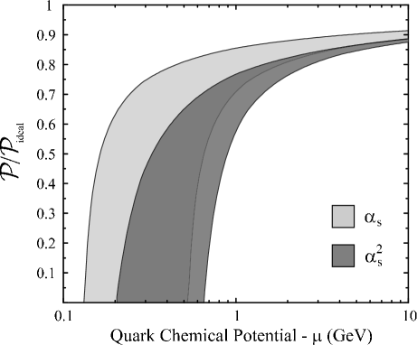
FIG. 1.: Perturbative result for the pressure of a degenerate quark-gluon plasma as a function of the quark chemical potential $\mu$ truncated at order $\alpha_{s}$ and $\alpha_{s}^{2}$. Bands correspond to variation of the renormalization scale $\mu\leq\Lambda\leq 4\mu$.

Note that the perturbative expansion of the thermodynamical potential is an expansion in $\alpha_{s}$ with coefficients that are polynomial in $\log(\alpha_{s})$ and that the logarithms of $\alpha_{s}$ are due to the effect of plasmons. To properly assess the convergence of the weak coupling expansion of the thermodynamics potential at $T=0$ and $\mu\neq 0$, we need to determine the order $\alpha_{s}^{3}$ contribution. While this would be a very complicated calculation, it can be obtained since the entire power series in $\alpha_{s}$ can be calculated using diagrammatic methods [19, 20]. This is in contrast to the high-temperature case where non-perturbative methods are required at order $\alpha_{s}^{3}$ due to infrared divergences associated with the screening of static magnetic gluons [21].

III HDL Free Energy

The weak-coupling expansion is an expansion about an ideal gas of massless particles and the lack of convergence suggests a reorganization of the perturbative series to improve the convergence and reduce the scale dependence. One possibility is to use HDLpt which is the analog of hard-thermal-loop perturbation theory (HTLpt) in the case of large chemical potentials. In HDLpt, one uses effective propagators and vertices that include plasma effects such as propagation of massive quasiparticles, screening, and Landau-damping. Thus the expansion point of HDLpt is that of ideal gas of massive particles. In the case of zero chemical potential and high temperature, this way of reorganizing the perturbative expansion has dramatically improved the convergence and reduced the renormalization scale dependence [9, 10, 11, 12].

At one-loop, HDLpt approximates the high-density phase of QCD by a gas of non-interacting massive quasiparticles. The one-loop HDL free energy for an $SU(N_{c})$ gauge theory with $N_{f}$ massless quarks is

$${\cal F} = (N_{c}^{2}-1)\left[(d-1){\cal F}_{T}+{\cal F}_{L}\right]$$ (5)

$$\hskip 64.01869pt+N_{c}N_{f}{\cal F}_{q}+\Delta_{0}{\cal E}_{0}\;,$$

where $d=3-2\epsilon$ is the number of spatial dimensions and ${\cal F}_{T}$ and ${\cal F}_{L}$ are the contributions to the free energy from the transverse and longitudinal gluons, respectively[10]. ${\cal F}_{q}$ is the contribution to the free energy from each color and flavor of the quarks, and $\Delta_{0}{\cal E}_{0}$ is the leading-order vacuum-energy counterterm. The contributions from the transverse and longitudinal gluons are

$${\cal F}_{T} = {1\over 2}\hbox{$\sum$}\!\!\!\!\!\!\!\int_{P}\log\left[P^{2}+\Pi_{T}(P)\right]\;,$$ (6)

$${\cal F}_{L} = {1\over 2}\hbox{$\sum$}\!\!\!\!\!\!\!\int_{P}\log\left[p^{2}-\Pi_{L}(P)\right]\;,$$ (7)

where $\Pi_{T}(P)$ and $\Pi_{L}(P)$ are the transverse and longitudinal HDL gluon self-energies. The quark contribution ${\cal F}_{q}$ is

$${\cal F}_{q}=-\log\det\left[P\!\!\!\!/-\Sigma(P)\right]\;,$$ (8)

where $\Sigma(P)$ is the quark self-energy. The quark contribution can be rewritten as [10, 22]

$${\cal F}_{q} = -2\hbox{$\sum$}\!\!\!\!\!\!\!\int_{\{P\}}\log P^{2}-2\hbox{$\sum$}\!\!\!\!\!\!\!\int_{\{P\}}\log\left[{A_{S}^{2}-A_{0}^{2}\over P^{2}}\right]\;.$$ (9)

The functions $\Pi_{T}(P)$, $\Pi_{L}(P)$, $A_{0}(P)$, and $A_{S}(P)$ are defined by

$$\Pi_{T}(P) = {3m_{g}^{2}P^{2}\over(d-1)p^{2}}\left[{\cal T}_{P}-1+{p^{2}\over P^{2}}\right]\;,$$ (10)

$$\Pi_{L}(P) = 3m^{2}_{g}\left[1-{\cal T}_{P}\right]\;,$$ (11)

$$A_{0}(P) = iP_{0}-{m_{q}^{2}\over iP_{0}}{\cal T}_{P}\;,$$ (12)

$$A_{S}(P) = p+{m^{2}_{q}\over p}\left[1-{\cal T}_{P}\right]\;,$$ (13)

where $m_{g}$ and $m_{q}$ are the gluon and quark mass parameters respectively, and the function ${\cal T}_{P}$ is defined by

$${\cal T}_{P} = w(\epsilon)\int_{0}^{1}dc\;(1-c^{2})^{-\epsilon}{P_{0}^{2}\over P_{0}^{2}+p^{2}c^{2}}\;,$$ (14)

where the function $w(\epsilon)$ is

$$w(\epsilon) = {\Gamma({3\over 2}-\epsilon)\over\Gamma({3\over 2})\Gamma(1-\epsilon)}\;.$$ (15)

IV Zero Temperature and Finite Chemical Potential

In this section, we calculate the zero-temperature limit of the one-loop HDL free energy Eq. (5). The zero-temperature limit of the gluon contribution was calculated in Ref. [10], while the the zero-temperature limit of the quark contribution was calculated in Ref. [22] using three-dimensional expressions for the self-energies. Since we are using dimensional regularization in our calculations, we use $d$-dimensional expressions for them. To leading order in HDL perturbation theory, the difference can be absorbed in a redefinition of the renormalization scale $\Lambda$. For higher order calculations, it essential to use the $d$-dimensional expressions for the quark and gluon self-energies.

A Gluon contribution

Our original expression for the gluon contribution

$${\cal F}_{g}=(d-1){\cal F}_{T}+{\cal F}_{L}$$ (16)

to the free energy involves a sum over the discrete Matsubara frequencies $\omega_{n}=2\pi nT$. As $T\rightarrow 0$, the sum approaches an integral over the continuous energy $\omega$. The only scale in the resulting integral is $m_{g}$ and ${\cal F}_{g}$ is proportional to $m_{g}^{4}$ on dimensional grounds.

In the zero-temperature limit, the transverse free energy ${\cal F}_{T}$ becomes

$${\cal F}_{T} = {1\over 4\pi}\left({e^{\gamma}\Lambda^{2}\over 4\pi}\right)^{\epsilon}\int_{-\infty}^{\infty}\;d\omega$$ (18)

$$\hskip 14.22636pt\times\int_{\bf p}\log\left[p^{2}+\omega^{2}+\Pi_{T}(\omega,p)\right]\;.$$

Since $\Pi_{T}$ is a function of the combination $\omega/p$ only, it is convenient to rescale the energy $\omega\rightarrow p\omega$. Integrating over the angles of ${\bf p}$ and using the fact that the integrand is an even function of $\omega$, the integral reduces to

$${\cal F_{T}} = {1\over 2\pi}{\Omega_{d}\over{(2\pi})^{d}}\left({e^{\gamma}\Lambda^{2}\over 4\pi}\right)^{\epsilon}\int_{0}^{\infty}d\omega\int_{0}^{\infty}dp\;p^{d}$$ (20)

$$\hskip 14.22636pt\times\log\left[(1+\omega^{2})p^{2}+\Pi_{T}(\omega,1)\right]\;,$$

where $\Omega_{d}=2\pi^{d/2}/\Gamma(d/2)$ is the angular integral. The dimensionally regulated integral over $p$ can be evaluated analytically using Eq. (A.12) giving

$${\cal F}_{T} = {1\over 2\pi}{\Omega_{d}\over(2\pi)^{d}}{\Gamma\left({d+1\over 2}\right)\Gamma\left({1-d\over 2}\right)\over d+1}\left({e^{\gamma}\Lambda^{2}\over 4\pi}\right)^{\epsilon}$$ (22)

$$\hskip 14.22636pt\times\int_{0}^{\infty}d\omega\left[{\Pi_{T}(\omega,1)\over 1+\omega^{2}}\right]^{(d+1)/2}\;.$$

Expanding around $d=3$ and evaluating the resulting integral over $\omega$ numerically, we obtain

$${\cal F}_{T} = -{9\over 8\pi}m_{g}^{4}\left({e^{\gamma}\Lambda^{2}\over 12\pi m_{g}^{2}}\right)^{\epsilon}{\Omega_{d}\over(2\pi)^{d}}$$ (24)

$$\hskip 14.22636pt\times\left[\left({1\over\epsilon}+{1\over 2}\right){\pi(8\log 2-5)\over 48}+0.116815\right]\;.$$

The longitudinal free energy ${\cal F}_{L}$ can be evaluated in the same manner and reads

$${\cal F}_{L} = -{9\over 8\pi}m_{g}^{4}\left({e^{\gamma}\Lambda^{2}\over 12\pi m_{g}^{2}}\right)^{\epsilon}{\Omega_{d}\over(2\pi)^{d}}$$ (26)

$$\hskip 14.22636pt\times\left[\left({1\over\epsilon}+{1\over 2}\right){\pi(1-\log 2)\over 3}+0.320878\right]\;.$$

The gluon contribution ${\cal F}_{g}$ to the free energy is obtained by inserting Eqs. (24) and (26) into Eq. (16)

$${\cal F}_{g} = -(N_{c}^{2}-1){9m_{g}^{4}\over 128\pi^{2}}\left[{1\over\epsilon}-2\log{m_{g}\over\Lambda}+1.24546\right]\;.$$ (27)

The pole in Eq (27) agrees with the one found in Ref. [10], but the finite term differs since $d$ was set equal to 3 in the expression for ${\cal T}_{P}$

B Quark contribution

The quark contribution Eq. (9) can be expanded in a power series of $m_{q}^{2}/\mu^{2}$. To second order in $m_{q}^{2}/\mu^{2}$, we obtain

$${\cal F}_{q} = -2\hbox{$\sum$}\!\!\!\!\!\!\!\int_{\{P\}}\log P^{2}-4m_{q}^{2}\hbox{$\sum$}\!\!\!\!\!\!\!\int_{\{P\}}{1\over P^{2}}+2m_{q}^{4}\hbox{$\sum$}\!\!\!\!\!\!\!\int_{\{P\}}$$ (29)

$$\;\times\left[{2\over P^{4}}-{1\over p^{2}P^{2}}+{2\over p^{2}P^{2}}{\cal T}_{P}-{1\over p^{2}P_{0}^{2}}\left({\cal T}_{P}\right)^{2}\right]\;.$$

Using the results for the zero-temperature limit of the different sum-integrals listed in the Appendix, Eq. (29) reduces to

$${\cal F}_{q} = -{\mu^{4}\over 12\pi^{2}}\left[1-6\left({m_{q}^{2}\over\mu^{2}}\right)+\left(6-\pi^{2}\right)\left({m_{q}^{2}\over\mu^{2}}\right)^{2}\right]\;.$$ (30)

We note that the quark contribution to the free energy is ultraviolet finite. The coefficient of the $m_{q}^{4}$ term is different from the one found in Refs. [10, 22], since $d$ was set equal to 3 in the expression for ${\cal T}_{P}$.

C One-loop free energy

The gluon contribution to the free energy Eq. (27) is ultraviolet divergent, while the quark contribution Eq. (29) is finite. The ultraviolet divergence is cancelled by the counterterm that was determined in Ref. [10]

$$\Delta_{0}{\cal E}_{0} = {9m_{g}^{4}\over 128\pi^{2}\epsilon}\;.$$ (31)

The total free energy is given by the sum of Eqs. (27), (30), and (31):

$${\cal F} = -{N_{c}N_{f}\mu^{4}\over 12\pi^{2}}\left[1-6\left({m_{q}^{2}\over\mu^{2}}\right)+\left(6-\pi^{2}\right)\left({m_{q}^{2}\over\mu^{2}}\right)^{2}\right]$$ (33)

$$\hskip 14.22636pt+(N_{c}^{2}-1){9m_{g}^{4}\over 64\pi^{2}}\left[\log{m_{g}\over\Lambda}-0.622732\right]\;.$$

Our leading order result for the thermodynamic functions depends on the gluon and quark mass parameters, and the renormalization scale $\Lambda$. These parameters are completely arbitrary in the sense that the dependence on them will be systematically subtracted out at higher orders. If higher order calculations were available, the masses could be determined by a variational principle giving rise to a self-consistent gap equation [9, 12]. In a one-loop calculation, we have little other choice than taking the weak-coupling expansion results for the gluon and quark masses. The gluon and quark masses are [23]

$$m_{g}^{2} = {2N_{f}\over 3}{\alpha_{s}(\Lambda)\over\pi}\mu^{2}\;,$$ (34)

$$m_{q}^{2} = {(N_{c}^{2}-1)\over 4N_{c}}{\alpha_{s}(\Lambda)\over\pi}\mu^{2}\;.$$ (35)

In the remainder of the paper we specialize to case $N_{c}=N_{f}=3$. The free energy (33) then reduces to

$${\cal F} = -{3\over 4\pi^{2}}\mu^{4}\left[1-4\left({\alpha_{s}\over\pi}\right)\right.$$ (37)

$$\;\left.-3\left(\log{\alpha_{s}\over\pi}+2\log{\mu\over\Lambda}+0.0209579\right)\left({\alpha_{s}\over\pi}\right)^{2}\right]\;.$$

Comparing the weak-coupling expansion Eq. (2) with the leading order HDL result Eq. (33), we note that the order-$\alpha_{s}$ term is over-included by a factor of two but the $\alpha_{s}^{2}\log\alpha_{s}$ term is included exactly. A next-to-leading order calculation in HDL perturbation theory would agree with the weak-coupling expansion at orders $\alpha_{s}$ and $\alpha_{s}^{2}\log\alpha_{s}$ if we identify the gluon and quark mass parameters with their weak-coupling expressions.

In Fig. 2, we show the leading-order HDL result for the free energy ${\cal F}$ normalized to that of an ideal gas. For comparison, we also show the next-to-leading order prediction from the QCD weak-coupling expansion as a grey band. The band is obtained by varying the renormalization scale $\Lambda$ by a factor of two around the central value $\Lambda=2\mu$. In this figure, we see that the HDLpt results also have a large variation with respect to the renormalization scale. Additionally, we see that the results for both $\Lambda=4\mu$ and $\Lambda=2\mu$ are both unphysical in that they predict negative quark number densities. If we add a requirement that the quark number density be positive we find that this requires $\Lambda\,\raisebox{-2.84544pt}{$\stackrel{{\scriptstyle<}}{{\sim}}$}\,1.6\mu$. We will use this as the lower bound for $\Lambda$ in the plots of the mass-radius relation in the next section.

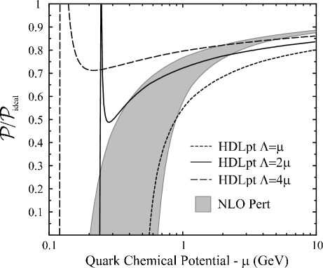
FIG. 2.: Leading-order HDLpt result for the pressure of a degenerate quark-gluon plasma as a function of chemical potential $\mu$. The NLO weak-coupling expansion result is shown as a grey band. Band corresponds to variation of the renormalization scale $\mu\leq\Lambda\leq 4\mu$.

Note that the requirement that $\Lambda\,\raisebox{-2.84544pt}{$\stackrel{{\scriptstyle<}}{{\sim}}$}\,1.6\mu$ may have some physical basis since the scale of the coupling constant should be related to the average momentum exchange of two quarks on the Fermi surface. At zero temperature the largest momentum exchange possible is $2\mu$ and the smallest momentum exchange is of the order of the superconducting gap $\phi$. Therefore, the scale for the coupling constant should be in the range $\phi\,\raisebox{-2.84544pt}{$\stackrel{{\scriptstyle<}}{{\sim}}$}\;\Lambda<2\mu$ so that the choice of $\Lambda\sim 1.6\mu$ is not unreasonable.

V Mass-Radius relationship

The mass-radius relationship for a non-rotating spherically symmetric star is obtained by solving the Tolman-Oppenheimer-Volkov (TOV) equations [24] for the mass $M$ and the pressure (${\cal P}=-{\cal F}$) as a function of the radial distance from the center:

$${dM\over dr} = 4\pi r^{2}\tilde{\cal E}(r)\;$$ (38)

$${d{\cal P}\over dr} = -{G\over r^{2}c^{2}}\left[\tilde{\cal E}(r)+\tilde{\cal P}(r)\right]\left[M(r)+4\pi r^{3}\tilde{\cal P}(r)\right]$$ (40)

$$\hskip 14.22636pt\times\left[1-{2GM(r)\over c^{2}r}\right]^{-1}\;,$$

where $G$ is Newton’s constant, $c$ is the speed of light, $\tilde{\cal E}={\cal E}/c^{2}$, and $\tilde{\cal P}={\cal P}/c^{2}$.

In this work we will ignore the presence of the nuclear phase of matter which is expected to undergo a first-order phase transition to the quark-matter phase. A more detailed study would include the effects of the nuclear phase on the mass-radius relationship; however, our goal here is only to show that both standard perturbation theory and HDLpt have large theoretical uncertainties related to the renormalization scale dependence. The most plausible scenario is that there will not be “naked” quark stars, but instead there will be neutron stars with a very compact quark-matter core and a thick outer layer of normal nuclear matter.

FIG. 3.: Mass-radius relation for a quark star with $\Lambda/\mu=1.6$ and $\Lambda/\mu=1$. The weak-coupling results for the same choice of renormalization scales are shown as dashed lines. $M_{\odot}=1.989\times 10^{30}$ kg is the mass of our sun.

In Fig. 3, we show the mass-radius relationship obtained by solving the TOV equations numerically for $\Lambda/\mu=1.6$ and $\Lambda/\mu=1$. For comparison, we also show the QCD weak-coupling expansion results for the same choice of renormalization scale as dashed lines. As can be seen from this figure there is a large variation in the mass-radius relationship as the renormalization scale is varied over even this rather limited range of $\mu\leq\Lambda\leq 1.6\,\mu$. Using this range, we find that using the HDLpt equation of state (37) that $R_{\rm max}\sim 3.4-10.9$ km and $M_{\rm max}\sim 0.6-2.12\,M_{\odot}$. With this same range we find that using the perturbative equation of state (2) that $R_{\rm max}\sim 2.4-5.6$ km and $M_{\rm max}\sim 0.42-0.95\,M_{\odot}$.

VI Discussion

In this paper, we have calculated the free energy of cold dense quark matter to leading order in HDL perturbation theory (HDLpt). The predictions of HDLpt depend on a renormalization scale $\Lambda$ that arises both from running of the coupling constant and from the renormalization of the additional ultraviolet divergences that are introduced by the HDLpt reorganization of perturbation theory. It is possible to separate these two effects by introducing two renormalization scales $\Lambda_{3}$ and $\Lambda_{4}$ as done in Ref. [10], and these scales are associated with the soft scale and hard scale, respectively. For simplicity we have chosen not to distinguish between the two and have simply set $\Lambda_{3}=\Lambda_{4}$.

We then used the HDLpt equation of state as input to the TOV equations in order to determine the mass-radius relationship of quark stars. We find that the large scale dependence of the HDLpt and weak-coupling expansion equations of state lead to large theoretical uncertainties in the quark star mass-radius relationship. In the case of the weak-coupling expansion, the expansion only seems to be under control for $\mu>5$ GeV. For HDLpt, the scale dependence is larger for all values of $\mu$ and without a next-to-leading order HDLpt calculation it is not possible to draw conclusions about the convergence of the series. In addition, the choices $\Lambda=4\mu$ and $\Lambda=2\mu$ lead to rather unphysical predictions as can be seen in Fig. 2. In order to eliminate these we were forced to further restrict the range of renormalization scales considered to $\mu\leq\Lambda\leq 1.6\,\mu$. The failure of both HDLpt and the weak-coupling expansion to reliably describe the finite-density QCD equation of state for $\mu$ between 300 MeV and 1 GeV is troubling since this is the range which is important for determining the mass-radius relationship for a quark star.

As mentioned in Section II, it possible that a computation of the order $\alpha_{s}^{3}$ contribution to the finite-density QCD equation of state could remove some of the theoretical uncertainties resulting from the use of the weak-coupling expansion result. Despite the fact that this would be a rather difficult task it seems that this calculation is required in order to draw more firm conclusions about the QCD equation of state. However, even if this calculation were available, the presence of a non-perturbative contribution from a color-superconducting phase of QCD in this range of quark chemical potential introduces additional theoretical uncertainties. Perturbative results extended down to this range of quark chemical potential give gaps on the order of $\phi\sim$ 30-100 MeV. Since the gap gives a relative contribution of the order of $\phi^{2}/\mu^{2}$ this could translate into a relative modification of the equation of state between 1% and 10%.

A very challenging problem would be to calculate the next-to-leading order correction to the free energy in HDLpt. If the next-to-leading order correction turns out to be small for relevant values of the chemical potential, the results obtained in the present work can be trusted. However, it would seem more prudent to compute the order $\alpha_{s}^{3}$ contribution in the weak-coupling expansion since the finite-density perturbation series does not seem to suffer from the same problems (oscillation and lack of convergence) as the finite-temperature perturbation series.

A

In the imaginary-time formalism for thermal field theory, the 4-momentum $P=(P_{0},{\bf p})$ is Euclidean with $P^{2}=P_{0}^{2}+{\bf p}^{2}$. The Euclidean energy $p_{0}$ has discrete values: $P_{0}=2n\pi T$ for bosons and $P_{0}=(2n+1)\pi T+\mu$ for fermions, where $n$ is an integer and $\mu$ is the chemical potential. Loop diagrams involve sums over $P_{0}$ and integrals over ${\bf p}$. With dimensional regularization, the integral is generalized to $d=3-2\epsilon$ spatial dimensions. We define the dimensionally regularized sum-integral by

$$\hbox{$\sum$}\!\!\!\!\!\!\!\int_{P} \equiv \left(\frac{e^{\gamma}\Lambda^{2}}{4\pi}\right)^{\epsilon}\;T\sum_{P_{0}=2n\pi T}\>\int{d^{3-2\epsilon}p\over(2\pi)^{3-2\epsilon}}\;,$$ (A.1)

$$\hbox{$\sum$}\!\!\!\!\!\!\!\int_{\{P\}} \!\!\!\!\equiv \!\!\left(\frac{e^{\gamma}\Lambda^{2}}{4\pi}\right)^{\epsilon}\;T\sum_{P_{0}=(2n+1)\pi T+\mu}\>\int{d^{3-2\epsilon}p\over(2\pi)^{3-2\epsilon}}\;,$$ (A.2)

where $3-2\epsilon$ is the dimension of space and $\Lambda$ is an arbitrary momentum scale. The factor $(e^{\gamma}/4\pi)^{\epsilon}$ is introduced so that, after minimal subtraction of the poles in $\epsilon$ due to ultraviolet divergences, $\Lambda$ coincides with the renormalization scale of the $\overline{\rm MS}$ renormalization scheme.

1 Simple one-loop sum-integrals

The simple fermionic sum-integrals required in our calculations are

$$\hbox{$\sum$}\!\!\!\!\!\!\!\int_{\{P\}}\log P^{2} = {2\mu^{4}\over 3(4\pi)^{2}}\;,$$ (A.3)

$$\hbox{$\sum$}\!\!\!\!\!\!\!\int_{\{P\}}{1\over P^{2}} = -{2\mu^{2}\over(4\pi)^{2}}\;,$$ (A.4)

$$\hbox{$\sum$}\!\!\!\!\!\!\!\int_{\{P\}}{1\over(P^{2})^{2}} = {1\over(4\pi)^{2}}\left({\Lambda\over 4\pi\mu}\right)^{2\epsilon}\left[{1\over\epsilon}+2\log(2\pi)\right]\;,$$ (A.5)

$$\hbox{$\sum$}\!\!\!\!\!\!\!\int_{\{P\}}{1\over p^{2}P^{2}} = {2\over(4\pi)^{2}}\left({\Lambda\over 4\pi\mu}\right)^{2\epsilon}$$ (A.7)

$$\hskip 14.22636pt\times\left[{1\over\epsilon}+2+2\log(2\pi)\right]\;.$$

These sum-integrals can be calculated by standard contour methods.

2 One-loop HDL sum-integrals

The one-loop fermionic sum-integrals involving the HDL function ${\cal T}_{P}$ are

$$\hbox{$\sum$}\!\!\!\!\!\!\!\int_{\{P\}}{1\over p^{2}P^{2}}{\cal T}_{P} = {2\over(4\pi)^{2}}\left({\Lambda\over 4\pi\mu}\right)^{2\epsilon}$$ (A.9)

$$\times\left[\log 2\left({1\over\epsilon}+3\log 2+2\log\pi\right)+{\pi^{2}\over 6}\right]\;,$$

$$\hbox{$\sum$}\!\!\!\!\!\!\!\int_{\{P\}}{1\over p^{2}P_{0}^{2}}\left({\cal T}_{P}\right)^{2} = {4\log 2\over(4\pi)^{2}}\left({\Lambda\over 4\pi\mu}\right)^{2\epsilon}$$ (A.11)

$$\times\left[{1\over\epsilon}+3\log 2+2\log\pi\right]\;.$$

These sum-integrals can be calculated using the methods developed in Ref. [11].

3 Integrals

In order to calculate the zero-temperature limit of ${\cal F}_{g}$, we need the following integral

$$\int_{0}^{\infty}dp\;p^{\alpha}\log(p^{2}+m^{2}) = {\Gamma\left({\alpha+1\over 2}\right)\Gamma\left({1-\alpha\over 2}\right)\over\alpha+1}m^{\alpha+1}\,.$$ (A.12)

REFERENCES

- [1] J.J. Drake, et. al., astro-ph/0204159.
- [2] F. Wilczek, Nucl.Phys. A663, 257 (2000).
- [3] E.S. Fraga, R.D. Pisarski, J.Schaffner-Bielich, Phys. Rev. D 63, 121702 (2001).
- [4] H. Satz, Phys. Lett. B 113, 245 (1982); J. Cleymans, R.V. Gavai, E. Suhonen, Phys. Rep. 130, 217 (1986).
- [5] A. Peshier, B. Kämpfer, and G. Soff, Phys. Rev. C 61, 045203 (2000); hep-ph/0106090.
- [6] P. Arnold and C. Zhai, Phys. Rev. D 50, 7603 (1994); Phys. Rev. D 51, 1906 (1995);
- [7] B. Kastening and C. Zhai, Phys. Rev. D 52, 7232 (1995).
- [8] E. Braaten and A. Nieto, Phys. Rev. Lett. 76, 1417 (1996); Phys. Rev. D 53, 3421 (1996).
- [9] F. Karsch, A. Patkós, and P. Petreczky, Phys. Lett. B 401, 69 (1997).
- [10] J.O. Andersen, E. Braaten and M. Strickland, Phys. Rev. Lett. 83, 2139 (1999); Phys. Rev. D 61, 014017 (2000).
- [11] J.O Andersen, E. Braaten, E. Petitgirard, and M. Strickland, hep-ph/0205085.
- [12] J. O. Andersen, E. Braaten and M. Strickland, Phys. Rev. D 63, 105008 (2001); J. O. Andersen and M. Strickland, Phys. Rev. D 64, 105012 (2001).
- [13] J.-P. Blaizot, E. Iancu, and A. Rebhan, Phys. Rev. Lett. 83, 2906 (1999); Phys. Lett. B 470, 181 (1999).
- [14] J.-P. Blaizot, E. Iancu, and A. Rebhan, Phys. Rev. D 63, 65003 (2001)
- [15] B.A. Freedman and L. McLerran, Phys. Rev. D 16, 1130 (1977); Phys. Rev. D 16, 1147 (1977); Phys. Rev. D 16, 1168 (1977); Phys. Rev. D 16, 1108 (1978).
- [16] V. Baluni, Phys. Rev. D 17, 2092, (1977).
- [17] Particle Data Group, D.E. Groom et al., Eur. J. Phys. C 15, 1 (2000).
- [18] G. Rodrigo and A. Santamaria, Phys. Lett. B 313, 441 (1993).
- [19] D. T. Son, Phys. Rev. D 59, 105020 (1999).
- [20] R. D. Pisarski D. H. Rischke, Phys. Rev. Lett. 37 (1999).
- [21] A. D. Linde. Phys. Lett. B96, 289 (1980).
- [22] R. Baier and K. Redlich, Phys. Rev. Lett. 84, 2100 (2000).
- [23] V. V. Klimov, Sov. Phys. JETP 55, 199 (1982); H. A. Weldon, Phys. Rev. D 26, 1394 (1982).
- [24] H. Heiselberg and M. Hjort-Jensen, Phys. Rep. 328, 237 (2000).