THEORY STATUS OF $\varepsilon^{\prime}/\varepsilon$ 

Abstract

I shortly review the present status of the theoretical calculations of $\varepsilon^{\prime}/\varepsilon$ and the comparison with the present experimental results. I discuss the role of higher order chiral corrections and in general of non-factorizable contributions for the explanation of the $\Delta I=1/2$ selection rule and direct CP violation in kaon decays. Still lacking satisfactory lattice calculations, analytic methods and phenomenological approaches are helpful in understanding correlations among theoretical effects and experimental data. Substantial progress from lattice QCD is expected in the coming years.

1 Introduction

The results obtained in the last few years by the NA48 [1] and the KTeV [2] collaborations have marked a great experimental achievement, establishing some 35 years after the discovery of CP violation in the neutral kaon system [3] the existence of a much smaller violation acting directly in the decays:

$$\mathop{\mbox{Re}}(\varepsilon^{\prime}/\varepsilon)=\left\{\begin{array}[]{ll}(15.3\pm 2.6)\times 10^{-4}&{\rm(NA48)}\\ (20.7\pm 2.8)\times 10^{-4}&{\rm(KTeV)}.\end{array}\right.$$ (1)

The average of these results with the previous measurements by the NA31 collaboration at CERN and by the E731 experiment at Fermilab gives

$$\mathop{\mbox{Re}}(\varepsilon^{\prime}/\varepsilon)=(17.2\pm 1.8)\times 10^{-4}.$$ (2)

While the Standard Model (SM) of strong and electroweak interactions provides an economical and elegant understanding of indirect ($\varepsilon$) and direct ($\varepsilon^{\prime}$) CP violation in term of a single phase, the detailed calculation of the size of these effects implies mastering strong interactions at a scale where perturbative methods break down. In addition, direct CP violation in $K\to\pi\pi$ decays arises from a detailed balance of two competing sets of contributions, which may hopelessly inflate the uncertainties related to the relevant hadronic matrix elements in the final outcome. All that makes predicting $\varepsilon^{\prime}/\varepsilon$ a complex and challenging task [4].

Just from the onset of the calculation the presence in the definition of $\varepsilon^{\prime}/\varepsilon$ , written as

$$\frac{\varepsilon^{\prime}}{\varepsilon}=\frac{1}{\sqrt{2}}\left\{\frac{\langle(\pi\pi)_{I=2}|{\cal H}_{W}|{K_{L}}\rangle}{\langle(\pi\pi)_{I=0}|{\cal H}_{W}|{K_{L}}\rangle}-\frac{\langle(\pi\pi)_{I=2}|{\cal H}_{W}|{K_{S}}\rangle}{\langle(\pi\pi)_{I=0}|{\cal H}_{W}|{K_{S}}\rangle}\right\}\ ,$$ (3)

of given ratios of isospin amplitudes warns us of a longstanding and still unsolved theoretical “problem”: the explanation of the $\Delta I=1/2$ selection rule.

The $\Delta I=1/2$ selection rule in $K\to\pi\pi$ decays is known since 45 years [5] and it states the experimental evidence that kaons are 400 times more likely to decay in the $I=0$ two-pion state than in the $I=2$ component ($\omega\equiv A_{2}/A_{0}\simeq 1/22$). This rule is not justified by any symmetry argument and, although it is common understanding that its explanation must be rooted in the dynamics of strong interactions, there is up to date no derivation of this effect from first principle QCD.

Given the possibility that common systematic uncertainties may a-priori affect the calculation of $\varepsilon^{\prime}/\varepsilon$ and the $\Delta I=1/2$ rule (see for instance the present difficulties in calculating on the lattice the “penguin contractions” for CP violating as well as for CP conserving amplitudes [6]) a convincing calculation of $\varepsilon^{\prime}/\varepsilon$ must involve at the same time a reliable explanation of the $\Delta I=1/2$ selection rule. Both observables indicate the need of large corrections to factorization in the evaluation of the four-quark hadronic transitions. Among these corrections Final State Interactions (FSI) play a substantial role. However, FSI alone are not enough to account for the large ratio of the $I=0$ over $I=2$ amplitudes. Other sources of large non-factorizable corrections are therefore needed for the CP conserving amplitudes [4, 8], which might affect the determination of $\varepsilon^{\prime}/\varepsilon$ as well. As a consequence, a self-contained calculation of $\varepsilon^{\prime}/\varepsilon$ should also address the determination of the $K\to\pi\pi$ rates.

2 OPE: an “effective” approach

The Operator Product Expansion (OPE) provides us with a very effective way to address the calculation of hadronic transitions in gauge theories. The integration of the “heavy” gauge and matter fields allows us to write the relevant amplitudes in terms of the hadronic matrix elements of effective quark operators and of the corresponding Wilson coefficients (at a scale $\mu$), which encode the information about those dynamical degrees of freedom which are heavier than the chosen renormalization scale. According to the SM flavor structure the $\Delta S=1$ transitions are effectively described by

$${\cal H}_{\Delta S=1}=\frac{G_{\rm F}}{\sqrt{2}}V_{ud}\,V^{*}_{us}\sum_{i}\Bigl{[}{z_{i}}(\mu)+{\tau}\ {y_{i}}(\mu)\Bigr{]}{Q_{i}}(\mu)\ .$$ (4)

The entries $V_{ij}$ of the $3\times 3$ Cabibbo-Kobayashi-Maskawa (CKM) matrix describe the flavour mixing in the SM and ${\tau}=-{V_{td}V_{ts}^{*}}/V_{ud}V_{us}^{*}$. For $\mu<m_{c}$ ($q=u,d,s$), the relevant quark operators are:

$$\begin{array}[]{lcl}\left.\begin{array}[]{lcl}{Q_{1}}&=&\left(\overline{s}_{\alpha}u_{\beta}\right)_{\rm V-A}\left(\overline{u}_{\beta}d_{\alpha}\right)_{\rm V-A}\\[4.30554pt] {Q_{2}}&=&\left(\overline{s}u\right)_{\rm V-A}\left(\overline{u}d\right)_{\rm V-A}\end{array}\right\}&&\mbox{Current-Current}\\[17.22217pt] \left.\begin{array}[]{lcl}{Q_{3,5}}&=&\left(\overline{s}d\right)_{\rm V-A}\sum_{q}\left(\overline{q}q\right)_{\rm V\mp A}\\[4.30554pt] {Q_{4,6}}&=&\left(\overline{s}_{\alpha}d_{\beta}\right)_{\rm V-A}\sum_{q}(\overline{q}_{\beta}q_{\alpha})_{\rm V\mp A}\end{array}\right\}&&\mbox{Gluon ``penguins''}\\[17.22217pt] \left.\begin{array}[]{lcl}{Q_{7,9}}&=&\frac{3}{2}\left(\overline{s}d\right)_{\rm V-A}\sum_{q}\hat{e}_{q}\left(\overline{q}q\right)_{\rm V\pm A}\\[4.30554pt] {Q_{8,10}}&=&\frac{3}{2}\left(\overline{s}_{\alpha}d_{\beta}\right)_{\rm V-A}\sum_{q}\hat{e}_{q}(\overline{q}_{\beta}q_{\alpha})_{\rm V\pm A}\end{array}\right\}&&\mbox{Electroweak ``penguins''}\end{array}$$ (5)

Current-current operators are induced by tree-level W-exchange whereas the so-called penguin (and “box”) diagrams are generated via an electroweak loop. Only the latter “feel” all three quark families via the virtual quark exchange and are therefore sensitive to the weak CP phase. Current-current operators control instead the CP conserving transitions. This fact suggests already that the connection between $\varepsilon^{\prime}/\varepsilon$ and the $\Delta I=1/2$ rule is by no means a straightforward one.

Using the effective $\Delta S=1$ quark Hamiltonian we can write $\varepsilon^{\prime}/\varepsilon$ as

$$\frac{{\varepsilon^{\prime}}}{\varepsilon}=e^{i\phi}\frac{G_{\rm F}\omega}{2|\epsilon|\mathop{\mbox{Re}}{A_{0}}}\>{\mbox{Im}\,\lambda_{t}}\>\>\left[{\Pi_{0}}-\frac{1}{\omega}\>{\Pi_{2}}\right]$$ (6)

where

$$\begin{array}[]{lcl}{\Pi_{0}}&=&\frac{1}{{\cos\delta_{0}}}\sum_{i}{y_{i}}\,\mathop{\mbox{Re}}\langle Q_{i}\rangle_{0}\ (1-{\Omega_{\rm IB}})\\[4.30554pt] {\Pi_{2}}&=&\frac{1}{{\cos\delta_{2}}}\sum_{i}{y_{i}}\,\mathop{\mbox{Re}}\langle Q_{i}\rangle_{2}\quad,\end{array}$$ (7)

and $\langle Q_{i}\rangle\equiv\langle\pi\pi|Q_{i}|K\rangle$. The rescattering phases $\delta_{0,2}$ can be extracted from elastic $\pi$-$\pi$ scattering data[7] and are such that $\cos\delta_{0}\simeq 0.8$ and $\cos\delta_{2}\simeq 1$. Given that the phase of $\varepsilon$ ($\theta_{\varepsilon}$) is approximately $\pi/4$, as well as the difference $\delta_{0}-\delta_{2}$, the $\varepsilon^{\prime}/\varepsilon$ phase $\phi=\frac{\pi}{2}+{\delta_{2}}-{\delta_{0}}-\theta_{\varepsilon}$ turns out to be consistent with zero. While $G_{\rm F}$, $\omega$, $|\varepsilon|$ and $\mathop{\mbox{Re}}A_{0}$ are precisely determined by experimental data, the first source of uncertainty that we encounter in eq. 6 is the value of $\mathop{\mbox{Im}}\lambda_{t}\equiv\mathop{\mbox{Im}}(V_{ts}^{*}V_{td})$, the combination of CKM elements which measures CP violation in $\Delta S=1$ transitions. The determination of $\mathop{\mbox{Im}}\lambda_{t}$ depends on B-physics constraints and on $\varepsilon$ [9]. In turn, the fit of $\varepsilon$ depends on the theoretical determination of $B_{K}$, the $\bar{K}^{0}-K^{0}$ hadronic parameter, which should be self-consistently determined within every analysis. The theoretical uncertainty on $B_{K}$ was in the past the main component of the final uncertainty on $\mathop{\mbox{Im}}\lambda_{t}$. The improved determination of the unitarity triangle coming from B-factories and hadronic colliders [10] has weakened and will eventually lift the dependence of $\mathop{\mbox{Im}}\lambda_{t}$ on $B_{K}$, allowing for an experimental measurement of the latter from $\varepsilon$ . Within kaon physics, the decay $K_{L}\to\pi^{0}\nu\bar{\nu}$ gives the cleanest “theoretical” determination of $\mathop{\mbox{Im}}\lambda_{t}$, albeit representing a great experimental challenge. At present, a typical range of values for $\mathop{\mbox{Im}}\lambda_{t}$ is $(0.94-1.60)\times 10^{-4}$ [11].

We come now to the quantities in the square brackets. While the calculation of the Wilson coefficients is well under control, thanks primarily to the work done in the early nineties by the Munich [12] and Rome [13] groups, the evaluation of the “long-distance” factors in eq. 7 is the crucial issue for the ongoing calculations. The isospin breaking (IB) parameter $\Omega_{\rm IB}$, gives at the leading-order (LO) in the chiral expansion a $positive$ correction to the $A_{2}$ amplitude (proportional to $A_{0}$ via the $\pi^{0}-\eta$ mixing) of about 0.13 [14]. At the next-to-leading order (NLO) the full inclusion of the $\pi^{0}-\eta-\eta^{\prime}$ mixing lift the value of $\Omega_{\rm IB}$ to $0.16\pm 0.03$ [15]. On the other hand, the complete NLO calculation of IB effects beyond the $\pi^{0}-\eta-\eta^{\prime}$ mixing (of strong and electromagnetic origin, among which the presence of $\Delta I=5/2$ transitions) involves a number of unknown NLO chiral couplings and is presently quite uncertain. Dimensional estimates show that IB effects may be large and affect $\varepsilon^{\prime}/\varepsilon$ sizeably in both directions  [16]. Although a partial cancellation of the indirect ($\Delta\omega$) and direct $\Delta\Omega_{\rm IB}$ NLO isospin breaking corrections in eq. 6 may reduce their final numerical impact on $\varepsilon^{\prime}/\varepsilon$ , we must await for further analyses in order to confidently assess their relevance. At present one may use $\Omega_{\rm IB}=0.10\pm 0.20$ [17, 18, 19] as a conservative estimate of the IB effects.

The final basic ingredient for the calculation of $\varepsilon^{\prime}/\varepsilon$ is the evaluation of the $K\to\pi\pi$ hadronic matrix elements of the quark operators in eq. 5. A simple albeit naive approach to the problem is the Vacuum Saturation Approximation (VSA), which is based on two drastic assumptions: the factorization of the four quark operators in products of currents and densities and the saturation of the intermediate states by the vacuum state. As an example:

$$\langle\pi^{+}\pi^{-}|Q_{6}|K^{0}\rangle = 2\ \langle\pi^{-}|\overline{u}\gamma_{5}d|0\rangle\langle\pi^{+}|\overline{s}u|K^{0}\rangle-2\ \langle\pi^{+}\pi^{-}|\overline{d}d|0\rangle\langle 0|\overline{s}\gamma_{5}d|K^{0}\rangle$$ (8)

$$+\ 2\left[\langle 0|\overline{s}s|0\rangle-\langle 0|\overline{d}d|0\rangle\right]\langle\pi^{+}\pi^{-}|\overline{s}\gamma_{5}d|K^{0}\rangle$$

The VSA does not exhibit a consistent matching of the renormalization scale and scheme dependences of the Wilson coefficients and it carries potentially large systematic uncertainties [4]. On the other hand it provides useful insights on the main features of the problem.

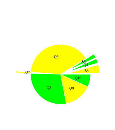
Figure 1: Anatomy of $\varepsilon^{\prime}/\varepsilon$ in the Vacuum Saturation Approximation. In light (dark) gray the positive (negative) contributions of the effective four-quark operators are shown with proportional weight.

A pictorial summary of the relative weights of the contributions of the various operators to $\varepsilon^{\prime}/\varepsilon$ , as obtained in the VSA, is shown in Fig. 1.

As we have already mentioned, CP violation involves loop-induced operators ($Q_{3}-Q_{10}$). From Fig. 1 one clearly notices the potentially large cancellation among the strong and electroweak sectors and the leading role played by the gluonic penguin operator $Q_{6}$ and the electroweak operator $Q_{8}$. Tipical range of values for $\varepsilon^{\prime}/\varepsilon$ , obtained using the VSA, are shown in Fig. 2 together with the three most updated predictions available before 1999 (when the first KTeV and NA48 results became known) [20, 21, 27]. The fact that the cancellation among the strong and electroweak sectors turns out to be quite effective (in the VSA) warns us about the possibility that the uncertainties in the determination of the relevant hadronic matrix elements may be largely amplified in the calculation of $\varepsilon^{\prime}/\varepsilon$ . It is therefore important to asses carefully the approximations related to the various parts of the calculations. In particular, the analysis of the problem suggests that factorization may be highly unreliable.

3 Beyond Factorization

Figure 2: The 1-$\sigma$ results of the NA31 and E731 Collaborations (early 90’s) are shown by the gray horizontal bands. The old München, Roma and Trieste theoretical predictions for $\varepsilon^{\prime}/\varepsilon$ are depicted by the vertical bars with their central values. For comparison, the VSA estimate is shown using two renormalization schemes.

The dark gray bars in Fig. 2 depict the results of three calculations of $\varepsilon^{\prime}/\varepsilon$ which are representative of approaches that (in principle) allow us to go beyond naive factorization. They are based from left to right on the large $N_{c}$ expansion [20, 22], on lattice regularization [21, 23], and on phenomenological modelling of low-energy QCD (the chiral quark model) [24, 25, 26, 27].

The experimental and theoretical scenarios have changed substantially after the first KTeV data and the subsequent NA48 results. Fig. 3 shows the present experimental world average for $\varepsilon^{\prime}/\varepsilon$ compared with the revised or new theoretical calculations that appeared during the last year. Without entering into the details of the results (for a short summary see [28]) they all represent attempts to incorporate non-perturbative information into the calculation of the hadronic matrix elements, whether their are based on the large $N_{c}$ expansion (München [29], Dortmund [30], Beijing [31], Taipei [32], Valencia [33]), phenomenological modelling of low-energy QCD (Dubna [34], Trieste [27, 35], Lund [36]), QCD Sum Rules (Montpellier [37]) or, finally, on lattice regularization (Roma [6], CP-PACS [38], RBC [39]).

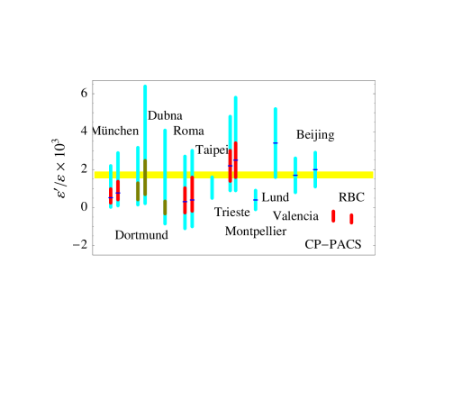
Figure 3: Recent theoretical calculations of $\varepsilon^{\prime}/\varepsilon$ are compared with the combined 1-$\sigma$ average of the NA31, E731, KTeV and NA48 results ($\varepsilon^{\prime}/\varepsilon$ = $17.2\pm 1.8\times 10^{-4}$), depicted by the gray horizontal band.

Overall most of the theoretical calculations are consistent with a non-vanishing positive effect in the SM (with the exception of the recent lattice results on which I will comment shortly).

At a closer look however, if we focus our attention on the central values, many of the predictions prefer the $10^{-4}$ regime, whereas only a few of them stand above $10^{-3}$. Is this just “noise” in the theoretical calculations? Without entering the many details on which the estimates are based, most of the aforementioned difference can be explained in terms of a single effect: the different size of the hadronic matrix element of the gluonic penguin $Q_{6}$ as obtained in the various approaches. In turn, this can be understood in terms of sizeable higher order chiral contributions (NLO in the $1/N_{c}$ expansion) to the $I=0$ amplitudes.

This effect was stigmatized well before the latest experimental round by the work of the Trieste group [26, 27], and appears clearly in the comparison of the leading $1/N_{c}$ and lattice results with the chiral quark model analysis in Fig. 2. The chiral quark model approach, together with the fit of the CP conserving amplitudes which normalizes phenomenologically the matching and the model parameters, allows us to carry the calculation of the hadronic matrix elements beyond the leading order in the chiral expansion (including the needed local counterterms). Non-factorizable chiral contributions (missing in the leading $1/N_{c}$ or lattice calculations) were shown to produce a substantial enhancement of the $I=0$ transitions thus lifting the expectation of $\varepsilon^{\prime}/\varepsilon$ at the $10^{-3}$ level.

Since then a number of groups have attempted to improve the calculation of $K\to\pi\pi$ matrix elements in a model independent way. Table 1 presents a comparison of different calculations of the relevant matrix elements. Due to the leading role played by $Q_{6}$ and $Q_{8}$ we may write a simplified version of eq. 6,

$$\frac{\varepsilon^{\prime}}{\varepsilon}\approx 13\left(\frac{\Lambda_{\overline{MS}}^{(4)}}{340\ {\rm MeV}}\right)\mathop{\mbox{Im}}\lambda_{t}\left[\frac{110\ {\rm MeV}}{m_{s}\ (2\ {\rm GeV})}\right]^{2}\ \left[{B_{6}}(1-\Omega_{\rm IB})-0.4{B_{8}^{(2)}}\right]\ ,\vspace*{-1ex}$$ (9)

which although “not be used for any serious analysis” [29] gives an effective and practical way to test and compare different calculations.

The B-factors $B_{i}\equiv\left\langle Q_{i}\right\rangle/\left\langle Q_{i}\right\rangle_{\rm VSA}$ represent a convenient parametrization of the hadronic matrix elements, albeit tricky, in that their values are in general scale and renormalization-scheme dependent, and a spurious dependence on the quark masses is introduced in the result whenever quark densities are involved. The latter is the case for the $Q_{6}$ and $Q_{8}$ penguins. As a consequence the VSA normalization may vary from author to author thus introducing systematic ambiguities. By taking the VSA matrix elements at the scale $\mu=2$ GeV we obtain [4]

$$\begin{array}[]{lcl@{}}&&\left\langle(\pi\pi)_{2}|Q_{8}|K^{0}\right\rangle_{\rm VSA}=\sqrt{6}\ f\ m_{K}^{4}\ (m_{s}+m_{d})^{-2}\simeq 1.1\ {\rm GeV}^{3}\ ,\\[4.30554pt] &&\left\langle\pi\pi|Q_{6}|K^{0}\right\rangle_{\rm VSA}/\left\langle(\pi\pi)_{2}|Q_{8}|K^{0}\right\rangle_{\rm VSA}=-2\sqrt{2}\ (f_{K}-f_{\pi})/f_{\pi}\simeq-0.63\ ,\end{array}$$ (10)

where I have used $(m_{s}+m_{d})(2\ {\rm GeV})=110\ {\rm MeV}$ and the chiral value $f=86$ MeV for the octet decay constant.

It is known that $B_{6}$ and $B_{8}^{(2)}$ are perturbatively very weakly dependent on the renormalization scale [4]. Therefore it makes sense to compare the $B$’s obtained in different approaches, where the matrix elements $\left\langle Q_{i}\right\rangle$ are computed at different scales. The results for the relevant penguin matrix elements coming from various approaches are collected in Table 1, paying care to normalizing the data in a homogeneous way (as far as detailed information on definitions and renormalization schemes was available).

As a guiding information, taking $\mathop{\mbox{Im}}\lambda_{t}=1.3\times 10^{-4}$, the present experimental central value of $\varepsilon^{\prime}/\varepsilon$ is reproduced by $B_{6}\ (1-\Omega_{\rm IB})-0.4\ B_{8}^{(2)}\approx 1$.

Table 1: Comparison of various calculations of penguin matrix elements. The data marked by the star are rescaled by a factor $\sqrt{3/2}$, to account for a different definition of the isospin matrix elements.

Method	$B_{6}$ (NDR)		$B_{8}^{(2)}$ (NDR)
Lattice (DWF, $K\to\pi$)	$<0.3$		$\sim 0.9$	CP-PACS[38]
Lattice (DWF, $K\to\pi$)	$\sim 0.4$		$\sim 1$	RBC[39]
Lattice ($K\to\pi+\chi$PT)	$-$		$0.58\pm 0.06$ *	APE[40]
Lattice ($K\to\pi+\chi$PT)	$-$		$0.56\pm 0.07$ *	SPQcdR[41]
Lattice ($K\to\pi\pi$)	$-$		$0.64\pm 0.07$ *	SPQcdR[41]
Large $N_{c}$+LMD ($\chi$-limit)	$-$		$2.6\pm 0.8$ *	Marseille[42]
Dispersive+data ($\chi$-limit)	$-$		$2.5\pm 0.8$ *	Amherst[43]
Dispersive+data ($\chi$-limit)	$-$		$1.4\pm 0.6$	Lund[44]
Large $N_{c}$ + data	$1.0\pm 0.3$		$0.8\pm 0.2$	Munich[29]
NLO $1/N_{c}$ CHPT	$1.5\sim 1.7$		$0.4\sim 0.7$	Dortmund[30]
NLO $1/N_{c}$ ENJL ($\chi$-limit)	$2.9\pm 0.5$		$1.5\pm 0.2$	Lund[36]
NLO $\chi$QM + $\chi$PT	$1.5\pm 0.4$		$0.84\pm 0.04$	Trieste[27]
Large $N_{c}$ + FSI	$1.55\pm 0.10$		$0.92\pm 0.03$	Valencia[33]

The most important fact is the first evidence of a signal in lattice calculations of $\left\langle\pi|Q_{6}|K\right\rangle$, obtained by the CP-PACS [38] and RBC [39] collaborations. Both groups use the Domain Wall Fermion approach which allows to control the chiral symmetry on the lattice as a volume effect in a fifth dimension. This approach softens in principle the problem of large power subtractions which affects the lattice extraction of $I=0$ amplitudes (penguin contractions). Still only the $\left\langle\pi|Q_{i}|K\right\rangle$ transition is computed on the lattice and LO chiral perturbation theory is used to extrapolate it to the physical amplitude. The two groups obtain comparable values of the $Q_{6}$ and $Q_{8}$ matrix elements leading both to a negative $\varepsilon^{\prime}/\varepsilon$ (and do not agree on the CP conserving $I=0$ amplitude). On the other hand the calculations are at an early stage and do not include higher order chiral dynamics which may be responsible for the enhancement of $I=0$ amplitudes (as large $N_{c}$ approaches beyond LO and the Chiral Quark Model strongly suggest). The SPQcdR collaboration has reported a result for the $Q_{8}$ matrix element from direct calculation of the $K\to\pi\pi$ amplitude on the lattice. This result agrees with previous lattice data, albeit it does not yet include the chiral corrections relevant to quenching and to the extrapolation to the physical pion mass [41].

Among the analytic approaches important results have been obtained using data on spectral functions in connection with QCD sum rules and dispersive relations in the attempt to obtain model independent information on the relevant matrix elements. These approaches have produced as of today calculations of $Q_{8}$ (in the chiral limit) which are subtantially larger than the factorization (and lattice) results. While there is still disagreement among the different analysis, we must await the calculation of the $Q_{6}$ matrix element and a quantitative assessment of chiral breaking effects before drawing conclusions on these as well as lattice results.

Calculations which sofar have allowed for the determination of all relevant parameters, based on chiral perturbation theory and/or models of low-energy QCD, have shown the crucial role of higher order non-factorizable corrections in the enhancement of the $I=0$ matrix elements [27, 30, 33, 36]. Chiral loop corrections drive the final value of $\varepsilon^{\prime}/\varepsilon$ in the ballpark of the present data. However the calculation of higher order chiral effects cannot be fully accomplished in a model independent way due to the many unknown NLO local couplings. In the chiral quark model approach all needed local interactions are computed in terms of quark masses, meson decay constants and a few non-perturbative parameters as quark and gluon condensates. The latter are determined self-consistently in a phenomenological way via the fit of the CP conserving $K\to\pi\pi$ amplitudes, thus encoding the $\Delta I=1/2$ rule in the calculation [26, 27]. The analysis shows that the role of local counterterms is subleading to the chiral logs when using the Modified Minimal Subtraction (as opposed to the commonly used Gasser-Leutwyler prescription). The phenomenological fit is crucial in stabilizing the numerical prediction [27]. The fact that the model parameters (quark and gluon condesates, constituent quark mass) turn out to be in the expected range, shows that the explicitly included chiral (and $1/N$ gluon condensate) corrections represent the largest non-factorizable effect.

Among higher order corrections FSI play a leading role. As a matter of fact, one should in general expect an enhancement of $\varepsilon^{\prime}/\varepsilon$ with respect to the naive VSA due to FSI. As Fermi first argued [45], in potential scattering the isospin $I=0$ two-body states feel an attractive interaction, of a sign opposite to that of the $I=2$ components thus affecting the size of the corresponding amplitudes. This feature is at the root of the enhancement of the $I=0$ amplitude over the $I=2$ one and of the corresponding enhancement of $\varepsilon^{\prime}/\varepsilon$ beyond factorization. An attempt to resum these effects in a model independent way has been worked out by the authors of ref. [33], using a dispersive approach a la Omnès-Mushkelishvili [46, 47]. Their analysis shows that resummation does not substantially modify the one-loop perturbative result and, as it appears from Table 1, a 50% enhancement of the gluonic penguin matrix element is found over the factorized result. However, the calculation suffers from a sistematic uncertainty due to the indetermination of the off-shell amplitude which is identified with the large $N_{c}$ result [48]. Even when the authors in the most recent work match the dispersive resummation with the on-shell perturbative one-loop calculation, thus including $1/N_{c}$ effects, again a systematic uncertainty remains in the unknown polinomial parts of the local chiral counterterms. Therefore, a model-independent complete calculation of chiral loops for $K\to\pi\pi$ is still missing.

Finally, it has been recently emphasized [49] that cut-off based approaches should pay attention to higher-dimension operators which become relevant for matching scales below 2 GeV and may represent one of the largest sources of uncertainty in present calculations. The results of refs. [43, 44] include these effects. The calculations based on dimensional regularization may be safe if phenomenological input is used in order to encode in the relevant hadronic matrix elements the physics at all scales (this is done in the Trieste approach).

In summary, while model dependent calculations suggest no conflict between theory and experiment for $\varepsilon^{\prime}/\varepsilon$ , a precise and ”pristine” prediction of the observable is still quite ahead of us.

4 Outlook and Conclusions

Higher-order chiral corrections are taking the stage of $K\to\pi\pi$ physics. They are needed in order to asses the size of crucial parameters (as $\Omega_{\rm IB}$) and the effect of non-factorizable contributions in the penguin matrix elements.

Lattice, as a regularization of QCD, is the first-principle approach to the problem. However, lattice calculations still heavily depend on chiral perturbation theory [50]. Presently, very promising developments are being undertaken to circumvemt the technical and conceptual shortcomings related to the calculation of weak matrix elements [41, 51]. Among those are the Domain Wall Fermion approach [52] which allows us to decouple the chiral symmetry from the continuum limit, and the very interesting observation that the Maiani-Testa theorem [53] can be overcomed using the fact that lattice calculations are performed in finite volume [54], thus allowing for the direct calculation of the physical $K\to\pi\pi$ amplitude on the lattice. All these developments need a tremendous effort in machine power and in devising faster algorithms. Preliminary results for lattice calculations of both $\varepsilon^{\prime}/\varepsilon$ and the $\Delta I=1/2$ selection rule are already available and others are currently under way [41].

In the meantime analytical and semi-phenomenological approaches have been crucially helpful in driving the attention of the community on some systematic short-comings of ”first-principle” calculations. The amount of theoretical work triggered by the NA48 and KTeV data promises rewarding and perhaps exciting results in the forthcoming years.

References

- 1 . A. Lai et al. , Eur. Phys. J. C 22, 231 (2001); S. Giudici, these Proceedings.
- 2 . A. Alavi-Harati et al. , Phys. Rev. Lett. 83, 22 (1999); S. Giudici, in 1).
- 3 . J.H. Christenson et al. , Phys. Rev. Lett. 13, 138 (1964).
- 4 . S. Bertolini, J.O. Eeg and M. Fabbrichesi, Rev. Mod. Phys. 72, 65 (2000); A.J. Buras, Erice School Lectures 2000, hep-ph/0101336.
- 5 . M. Gell-Mann and A. Pais, Proc. Glasgow Conf. , 342 (1955).
- 6 . M. Ciuchini and G. Martinelli, Nucl. Phys. Proc. Suppl. 99B, 27 (2001).
- 7 . J. Gasser and U.G. Meissner, Phys. Lett. B 258, 219 (1991); E. Chell and M.G. Olsson, Phys. Rev. D 48, 4076 (1993).
- 8 . J.-M. Gérard and J. Weyers, Phys. Lett. B 503, 99 (2001); N.I. Kochelev and V. Vento, Phys. Rev. Lett. 87, 111601 (2001).
- 9 . M. Ciuchini et al. , JHEP 0107, 013 (2001).
- 10 . K. Kleinknecht, these Proceeedings.
- 11 . A.J. Buras, Proc. Kaon 2001 Conf., Pisa, Italy, hep-ph/0109197.
- 12 . A.J. Buras et al. , Nucl. Phys. B 370, 69 (1992); Nucl. Phys. B 400, 37 (1993); Nucl. Phys. B 400, 75 (1993); Nucl. Phys. B 408, 209 (1993).
- 13 . M. Ciuchini et al. , Phys. Lett. B 301, 263 (1993); Nucl. Phys. B 415, 403 (1994).
- 14 . J. Gasser and H. Leutwyler, Nucl. Phys. B 250, 465 (1985).
- 15 . G. Ecker et al. , Phys. Lett. B 467, 88 (2000).
- 16 . S. Gardner and G. Valencia, Phys. Lett. B 466, 355 (1999).
- 17 . S. Gardner and G. Valencia, Phys. Rev. D 62, 094024 (2000).
- 18 . K. Maltman and C. Wolfe, Phys. Lett. B 482, 77 (2000); Phys. Rev. D 63, 014008 (2001).
- 19 . V. Cirigliano, J.F. Donoghue and E. Golowich, Phys. Lett. B 450, 241 (1999); Phys. Rev. D 61, 093001 (2000); Phys. Rev. D 61, 093002 (2000); Eur. Phys. J. C 18, 83 (2000).
- 20 . A.J. Buras, M. Jamin and E. Lautenbacher, Phys. Lett. B 389, 749 (1996).
- 21 . Ciuchini et al. , Z. Phys. C 68, 239 (1995); Nucl. Phys. Proc. Suppl. 59, 149 (1997).
- 22 . W.A. Bardeen, A.J. Buras and J.M. Gerard, Nucl. Phys. B 293, 787 (1987).
- 23 . G. Martinelli, Proc. Kaon 99 Conf., Chicago, USA, hep-ph/9910237.
- 24 . S. Weinberg, Physica A, 96 (327)1979; A. Manhoar and H. Georgi, Nucl. Phys. B 234, 189 (1984).
- 25 . A. Pich and E. de Rafael, Nucl. Phys. B 358, 311 (1991).
- 26 . S. Bertolini et al. , Nucl. Phys. B 514, 63 (1998).
- 27 . S. Bertolini et al. , Nucl. Phys. B 514, 93 (1998); Phys. Rev. D 63, 056009 (2001).
- 28 . S. Bertolini, Proc. RADCOR 2000, Carmel, USA, eConf C000911, hep-ph/0101212.
- 29 . A.J. Buras, Proc. Kaon 99 Conf., Chicago, USA, hep-ph/9908395.
- 30 . T. Hambye et al. , Phys. Rev. D 58, 014017 (1998); Nucl. Phys. B 564, 391 (2000).
- 31 . Yue-Liang Wu, Phys. Rev. D 64, 016001 (2001).
- 32 . H.Y. Cheng, Chin. J. Phys. 38, 1044 (2000).
- 33 . E. Pallante and A. Pich, Phys. Rev. Lett. 84, 2568 (2000); Nucl. Phys. B 592, 294 (2000); E. Pallante, A. Pich and I. Scimemi, Nucl. Phys. B 617, 441 (2001).
- 34 . A.A. Bel’kov et al. , hep-ph/9907335.
- 35 . M. Fabbrichesi, Phys. Rev. D 62, 097902 (2000).
- 36 . J. Bijnens and J. Prades, JHEP 0006, 035 (2000).
- 37 . S. Narison, Nucl. Phys. B 593, 3 (2001).
- 38 . J. Noaki et al. , hep-lat/0108013.
- 39 . T. Blum et al. , hep-lat/0110075.
- 40 . A. Donini et al. , Phys. Lett. B 470, 233 (1999).
- 41 . G. Martinelli, Nucl. Phys. Proc. Suppl. 106, 98 (2002), hep-lat/0112011.
- 42 . M. Knecht, S. Peris and E. de Rafael, Phys. Lett. B 508, 117 (2001); S. Peris, hep-ph/0204181.
- 43 . V. Cirigliano, J.F. Donoghue, E. Golowich and K. Maltman, Phys. Lett. B 522, 245 (2001).
- 44 . J. Bijnens, E. Gamiz and J. Prades, JHEP 0110, 009 (2001).
- 45 . E. Fermi, Suppl. Nuovo Cim. 2, 17 (1955).
- 46 . N.I. Mushkelishvili, Singular Integral Equations (Noordhoff, Gronigen, 1953), p. 204; R. Omnès, Nuovo Cim. 8, 316 (1958).
- 47 . T.N. Truong, Phys. Lett. B 207, 495 (1988); U. Meissner, in “Perspectives in Nucl. Physics at Intermediate Energies” 385-398, Trieste 1991.
- 48 . A. J. Buras et al. , Phys. Lett. B 480, 80 (2000); M. Buechler et al. , Phys. Lett. B 521, 29 (2001).
- 49 . V. Cirigliano, J.F. Donoghue and E. Golowich, JHEP 0010, 048 (2000).
- 50 . M. Golterman and E. Pallante, Nucl. Phys. Proc. Suppl. 106, 335 (2002), hep-lat/0110183.
- 51 . C.T. Sachrajda, Proc. Lepton-Photon 2001, Roma, Italy, hep-ph/0110304.
- 52 . D. Kaplan, Phys. Lett. B 288, 342 (1992).
- 53 . L. Maiani and M. Testa, Phys. Lett. B 245, 585 (1990).
- 54 . L. Lellouch and M. Lüscher, Comm. Math. Phys. 219, 31 (2001).