Hadronic $\tau$ decay, the renormalization group, analiticity of the polarization operators and QCD parameters.

The ALEPH data on hadronic $\tau$-decay is throughly analysed in the framework of QCD. The perturbative calculations are performed in 1-4-loop approximation. The analytical properties of the polarization operators are used in the whole complex $q^{2}$ plane. It is shown that the QCD prediction for $R_{\tau}$ agrees with the measured value $R_{\tau}$ not only for conventional $\Lambda^{conv}_{3}=(618\pm 29)~{}MeV$ but as well as for $\Lambda^{new}_{3}=(1666\pm 7)~{}MeV$. The polarization operator calculated using the renormgroup has nonphysical cut $[-\Lambda^{2}_{3},0]$. If $\Lambda_{3}=\Lambda^{conv}_{3}$, the contribution of only physical cut is deficient in the explanation of the ALEPH experiment. If $\Lambda_{3}=\Lambda^{new}_{3}$ the contribution of nonphysical cut is very small and only the physical cut explains the ALEPH experiment. The new sum rules which follow only from analytical properties of polarization operators are obtained. Basing on the sum rules obtained, it is shown that there is an essential disagreement between QCD perturbation theory and the $\tau$-lepton hadronic decay experiment at conventional value $\Lambda_{3}$. In the evolution upwards to larger energies the matching of $r(q^{2})$ (Eq.(12)) at the masses $J/\psi$, $\Upsilon$ and $2m_{t}$ was performed. The obtained value $\alpha_{s}(-m^{2}_{z})=0.141\pm 0.004$ (at $\Lambda_{3}=\Lambda^{new}_{3}$) differs essentially from conventional value, but the calculation of the values $R(s)=\frac{\sigma(e^{+}e^{-}\to hadrons)}{\sigma(e^{+}e^{-}\to\mu^{+}\mu^{-})}$,   $R_{l}=\frac{\Gamma(Z\to hadrons)}{\Gamma(Z\to leptons)}$,   $\alpha_{s}(-3~{}GeV^{2})$,   $\alpha_{s}(-2.5~{}GeV^{2})$ does not contradict the experiments.

1 INTRODUCTION

The purpose of this work is to combine the analyticity requirements of QCD polarization operators with the renormalization group. This work is the continuation of works [1-3]. In the work [1] analytical properties of polarization operators were used to improve perturbation theory in QCD. In the works [2,3] the high precision data on hadronic $\tau$-decay obtained by the ALEPH [4], OPAL [5] and CLEO [6] Collaborations were analyzed in the framework of QCD. The analyticity requirements of the QCD polarization operators follow from the microcausality and the unitarity, therefore we have no doubts about them. On the other hand, the calculation according to renormgroup leads to appearance of nonphysical singularities. So, the one-loop calculation gives a nonphysical pole, while in the calculation in a larger number of loops the pole disappears, but a nonphysical cut appears, $[-\Lambda^{2}_{3},0]$. As will be shown, there are only two values of $\Lambda_{3}$, such that theoretical predictions of QCD for $R_{\tau,V+A}$ (formulae (23),(24) agree with the experimens [4-6]. These values are the following: one conventional value $\Lambda^{conv}_{3}=(618\pm 29)~{}MeV$ and the other value of $\Lambda_{3}$ is $\Lambda^{new}_{3}=(1666\pm 7)~{}MeV$. Only in these values of $\Lambda_{3}$ the predictions of QCD are consistent with the experiments [4-6]. As far as I know, the value $\Lambda_{3}=\Lambda^{new}_{3}$ was not considered before now If one simply puts out the nonphysical cut and leaves the conventional value $\Lambda^{conv}_{3}$, then the discrepancy between the theory and experiment will arise. As will be shown, if instead of the conventional value $\Lambda^{conv}_{3}$ one chooses the value $\Lambda^{new}_{3}=(1565\pm 193)~{}MeV$ then only the physical cut contribution is enough to explain the experiment of the hadronic $\tau$-decay. . It is convenient to introduce the Adler function (11-13) instead of the polarization operator. The Adler function is an analytical function of $q^{2}$ in the whole complex $q^{2}$ plane with a cut along the positive $q^{2}$ semiaxes. We will use the renormgroup only for negative $q^{2}$, where the value $\alpha_{s}(q^{2})$ is real and positive. For other $q^{2}$ the value $\alpha_{s}(q^{2})$ becomes complex and is obtained by analytical continuation.

The plan of the paper is the following.

In Section 2 the formulae obtained in paper [3] are transformed to suitable for this paper form.

In Section 3 the values $\Lambda_{3}$ are found such that $R_{\tau,V+A}=3.475\pm 0.022$ (formula (24)).

In Section 4 we obtain new sum rules for polarization operator which follow only from analytical properties of the polarization operator. These sum rules imply that there is an essential discrepancy between perturbation theory in QCD and the experiment in hadronic $\tau$ decay at conventional value of $\Lambda_{3}$. The power corrections and instantons cannot eliminate this discrepancy.

Section 5 suggests the method of resolving these discrepancies. At $\Lambda_{3}=(1565\pm 193)~{}MeV$ the nonphysical cut gives no contribution into $R_{\tau,V+A}$ and the physical cut gives the experimentally observed value $R_{\tau,V+A}$. The previously derived sum rules make no sense if $\Lambda_{3}$ is as large.

In Section 6 we go over to larger energies. In the matching procedure we require continuity of $r(s)$ (Eq.(12)) [1] at masses $J/\psi$, $\Upsilon$ and $2m_{t}$ when going over from $n_{f}$ to $n_{f}+1$ flavours. The number of flavours on the cut is a good quantum number. At every point off the cut all flavours give a contribution. This follows from the dispersion relation for the Adler function. The continuity requirement off the cut when changing the number of flavours violates analytical properties of the polarization operator. Section 6 presents the results of the calculations in 1-4 loops for estimation of the precision of the calculations. In Sections 7-9 we compare the theory with experiment. In Section 7 the prediction of the function $R(s)$ is compared with experiments. The calculated values of the function $R(s)$ are in a very good agreement with the experiment (Tables 5,6) at $2\leq\sqrt{s}\leq 47.6GeV$ except for the resonance region.

In Section 8 we compare the calculated values of $\alpha_{s}(-3GeV^{2})$ and $\alpha_{s}(-2.5GeV^{2})$ with the values $\alpha_{s}(-3GeV^{2})$ and $\alpha_{s}(-2.5GeV^{2})$ obtained from the Gross-Llewellyn-Smith sum rule [7] and the Bjorken sum rule [8]. The results of the calculations are in agreement with the values obtained from the experiment using these sum rules.

Section 9 presents the calculation of $R_{l}=\frac{\Gamma(Z\to hadrons)}{\Gamma(Z\to leptons)}$. The obtained value $R_{l}$ does not contradict the experiment.

Section 10 is devoted to discussion on the analiticity $\alpha_{s}(q^{2})$. It is shown that the statement that $\alpha_{s}(0)=4\pi/\beta_{0}=1.396$ is valid only for one-loop calculations.

2 INITIAL FORMULAE

In this section the formulae obtained in the paper [3] are transformed to suitable for this paper form. We will consider three loop approximation thoroughly. Polarization operators of hadronic currents are defined by the formula

$$\Pi^{J}_{\mu\nu}(q)=i~{}\int e^{iqx}\langle 0\mid T~{}J_{\mu}(x)J^{+}_{\nu}(0)\mid 0\rangle d^{4}x=$$

$$=(q_{\mu}q_{\nu}-g_{\mu\nu}q^{2})\Pi^{(1)}_{J}(q^{2})+q_{\mu}q_{\nu}\Pi^{(0)}(q^{2})$$ (1)

where

$$J=V,A;~{}~{}V_{\mu}=\bar{u}\gamma_{\mu}d,~{}~{}A_{\mu}=\bar{u}\gamma_{\mu}\gamma_{5}d$$

Imaginary parts $\Pi^{(1)}_{J},\Pi^{(0)}_{J}$ are connected with the measured, so called spectral functions $v_{1}(s),a_{1}(s),a_{0}(s)$ by the formulae

$$v_{1}(s)/a_{1}(s)=2\pi~{}Im\Pi^{(1)}_{V/A}(s+i0)$$

$$a_{0}(s)=2\pi~{}Im\Pi^{(0)}_{A}(s+i0)$$ (2)

Functions $\Pi^{(1)}_{V/A}$ are analytical functions of $q^{2}$ with the cuts $[4m^{2}_{\pi},\infty]$ for $\Pi^{(1)}_{V}$ and $[9m^{2}_{\pi},\infty]$ for $\Pi^{(1)}_{A},a_{0}(s)=2\pi^{2}f^{2}_{\pi}\delta(s-m^{2}_{\pi}),f_{\pi}=130.7MeV$.

To get QCD predictions let us use the renormalization group equation in 3-loop approximation [9-10]

$$q^{2}\frac{\partial a}{\partial q^{2}}=-\beta^{(n_{f})}_{0}~{}a^{2}(1+b^{(n_{f})}_{1}a+b^{(n_{f})}_{2}~{}a^{2})$$ (3)

where

$$a(q^{2})=\frac{\alpha_{s}(q^{2})}{4\pi},~{}~{}\beta^{(n_{f})}_{0}=11-\frac{2}{3}n_{f},~{}~{}\beta^{(n_{f})}_{1}=51-\frac{19}{3}n_{f},$$

$$\beta^{(n_{f})}_{2}=2857-\frac{5033}{9}n_{f}+\frac{325}{27}n^{2}_{f},~{}~{}b^{(n_{f})}_{1}=\frac{2\beta^{(n_{f})}_{1}}{\beta^{(n_{f})}_{0}},~{}~{}b^{(n_{f})}_{2}=\frac{\beta_{2}^{(n_{f})}}{2\beta^{(n_{f})}_{0}}.$$ (4)

Here $n_{f}$ is the number of flavours.

Let us consider for the moment $n_{f}=3$ and omit the mark $n_{f}$. Find singularities of $a(q^{2})$. Integrate equation (3) [3]

$$\beta_{0}ln~{}\frac{q^{2}}{\mu^{2}}=-\int\limits^{a(q^{2})}_{a(\mu^{2})}\frac{da}{a^{2}(1+b_{1}a+b_{2}a^{2})}$$ (5)

Denote the value $q^{2}$ at which $a(q^{2})=\infty$ as $-\Lambda^{2}_{3}$. Then we get instead of eq.5:

$$\beta_{0}ln\Biggl{(}\frac{-q^{2}}{\Lambda^{2}_{3}}\Biggr{)}=\int\limits^{\infty}_{a(q^{2})}~{}\frac{da}{a^{2}(1+b_{1}a+b_{2}a^{2})}\equiv f(a)$$ (6)

According to the known value $a(-m^{2}_{\tau})$   $\Lambda^{2}_{3}$ is determined by the formula

$$\Lambda^{2}_{3}=m^{2}_{\tau}e^{-\frac{f(a(-m^{2}_{\tau}))}{\beta_{0}}}$$ (7)

The integral in the formula (6) is taken and the answer is written as

$$f(a)=\frac{1}{a}+b_{1}~{}lna-\frac{1}{\sqrt{b^{2}_{1}-4b_{2}}}\Biggl{[}\frac{1}{x^{2}_{1}}~{}ln(a-x_{1})-\frac{1}{x^{2}}~{}ln(a-x_{2})\Biggr{]}$$ (8)

where

$$x_{1,2}=\frac{-b_{1}\pm\sqrt{b^{2}_{1}-4b_{2}}}{2b_{2}}$$

At $\alpha_{s}(-m^{2}_{\tau})=0.355$  [3] we obtain $\Lambda^{2}_{3}=0.394GeV^{2}$.

The expansion of the function $f(a)$ in the Taylor series at large $a$ over $1/a$ is of the form

$$f(a)=\frac{1}{3b_{2}}~{}\frac{1}{a^{3}}-\frac{b_{1}}{4b^{2}_{2}}~{}\frac{1}{a^{4}}+\frac{(b^{2}_{1}-b_{2})}{5b^{3}_{2}}~{}\frac{1}{a^{5}}+0(\frac{1}{a^{6}})$$ (9)

It follows from eqs.(6-9) that the singularity $a(q^{2})$ at $q^{2}\to-\Lambda^{2}_{3}$ has the form [3]

$$a(q^{2})=\Biggl{(}-\frac{2\Lambda^{2}_{3}}{3\beta_{2}(q^{2}+\Lambda^{2}_{3})}\Biggr{)}^{1/3}$$ (10)

Since for massless quarks the contributions of $V$ and $A$ coincide, we will omit in all formulae the mark $J$. Introduce the Adler function

$$D(q^{2})=-q^{2}\frac{d\Pi(q^{2})}{dq^{2}}$$ (11)

It is convenient to write for three flavours

$$D(q^{2})=3(1+d(q^{2})),~{}~{}R(q^{2})=3(1+r(q^{2})),~{}\Pi(q^{2})=3(-ln(-q^{2}/\mu^{2})+p(q^{2}))$$

$$r(q^{2})=\frac{1}{\pi}Imp(q^{2})=\frac{1}{2\pi i}[p(q^{2}+i0)-p(q^{2}-i0)]$$ (12)

In 3-loop approximation for $\overline{MS}$ renormalization scheme function $d(q^{2})$ for negative $q^{2}$ is written as [11]:

$$d(q^{2})=4a(q^{2})(1+4d^{(n_{f})}_{1}a(q^{2})+16d^{(n_{f})}_{2}a(q^{2})^{2})$$ (13)

where

$$d^{(n_{f})}_{1}=1.9857-0.1153n_{f}$$

$$d^{(n_{f})}_{2}=18.244-4.216n_{f}+0.086n^{2}_{f}$$ (14)

Hereafter we will follow [3]

$$d(q^{2})=-q^{2}\frac{dp(q^{2})}{dq^{2}}$$ (15)

$$p(q^{2})=-\int~{}\frac{d(q^{2})}{q^{2}}dq^{2}$$ (16)

Using formula (3)

$$\frac{dq^{2}}{q^{2}}=-\frac{da}{\beta_{0}a^{2}(1+b_{1}a+b_{2}a^{2})}$$ (17)

we get for the function $p(q^{2})$ the expression

$$p(q^{2})=\frac{1}{\beta_{0}}~{}\int~{}\frac{d(a)da}{a^{2}(1+b_{1}a+b_{2}a^{2})}=\frac{1}{\beta_{0}b_{2}}~{}\int~{}\frac{d(a)da}{a^{2}(a-x_{1})(a-x_{2})}$$ (18)

After taking the integral (18) we get

$$p(a)=\frac{4}{\beta_{0}}lna+\frac{4}{\beta_{0}\sqrt{b^{2}_{1}-4b_{2}}}\left\{(\frac{1}{x_{1}}+4d_{1}+16d_{2}x_{1})ln(a-x_{1})-(\frac{1}{x_{2}}+4d_{1}+16d_{2}x_{2})ln(a-x_{2})\right\}$$ (19)

$x_{1}$, $x_{2}$ are determined by formula (8a).

The polarization operator is an analytical function with the cut $[0,\infty]$. The polarization operator calculated in 3-loop approximation has the physical cut $0<q^{2}<\infty$ and nonphysical one $-\Lambda^{2}_{3}<q^{2}<0$. The contribution of the physical cut in the value $R^{S=0}_{\tau,V+A}$ is equal to

$$R^{QCD}_{\tau,V+A}\Biggl{|}_{phys.cut}=6|V_{ud}|^{2}S_{EW}\int\limits^{m^{2}_{\tau}}_{0}\frac{ds}{m^{2}_{\tau}}(1-\frac{s}{m^{2}_{\tau}})^{2}(1+2\frac{s}{m^{2}_{\tau}})(1+r(s))ds+\Delta R^{(0)}_{\tau}$$ (20)

where $|V_{ud}|=0.9735\pm 0.0008$ is the Cabibbo-Kobayashi-Maskawa matrix element [12], $S_{EW}=1.0194\pm 0.040$ is the contribution of electroweak corrections [13].

$$\Delta R^{(0)}_{\tau}=-24\pi^{2}\frac{f^{2}_{\pi}m^{2}_{\pi}}{m^{2}_{\tau}}=-0.008.$$ (21)

is a small correction from the pion pole [3]. The nonphysical cut contribution is equal to

$$R^{(QCD)}_{\tau,V+A}\Biggl{|}_{nonphysicalcut}=6|V_{ud}|^{2}S_{EW}\int\limits^{0}_{-\Lambda^{2}_{3}}~{}\frac{ds}{m^{2}_{\tau}}(1-\frac{s}{m^{2}_{\tau}})^{2}(1+2\frac{s}{m^{2}_{\tau}})(1+r(s))ds$$ (22)

3 Finding of the value $\Lambda_{3}$

The value measured in the experiment is

$$R_{\tau,V+A}=\frac{B(\tau\to\nu_{\tau}+hadrons,~{}S=0)}{B(\tau\to e^{-}\bar{\nu}_{e}\nu_{\tau})}=$$

$$=6|V_{ud}|^{2}S_{EW}\int\limits^{m^{2}_{\tau}}_{0}\frac{ds}{m^{2}_{\tau}}(1-\frac{s}{m^{2}_{\tau}})^{2}\Biggl{[}(1+2\frac{s}{m^{2}_{\tau}})(v_{1}(s)+a_{1}(s)+a_{0}(s))-2\frac{s}{m^{2}_{\tau}}a_{0}(s)\Biggr{]}$$ (23)

For the value $R_{\tau,V+A}$ , the ALEPH [4], OPAL [5] and CLEO [6] Collaborations had obtained

$$R_{\tau,V+A}=3.475\pm 0.022$$ (24)

Here new value of $R_{\tau,S}$ [14,15] is taken into account.

$$R_{\tau,S}=0.161\pm 0.007$$ (25)

The convenient way to calculate the $R_{\tau}$ in QCD is to transform the integral in the complex $s$ plane [16-19] around the circle $|s|=m^{2}_{\tau}$ and thus getting a satisfactory agreement with the experiment.

$$R_{\tau,V+A}=6\pi i|V_{ud}|^{2}S_{EW}\oint_{|s|=m^{2}_{\tau}}~{}\frac{ds}{m^{2}_{\tau}}(1-\frac{s}{m^{2}_{\tau}})^{2}(1+2\frac{s}{m^{2}_{\tau}})(1+2\frac{s}{m^{2}_{\tau}})\Pi(s)+\Delta R^{(0)}_{\tau}$$ (26)

There are two values of $\Lambda_{3}$, such that $R_{\tau,V+A}=3.475\pm 0.022$ (Eq.24). These values are: conventional value

$$\Lambda^{conv}_{3}=618\pm 29MeV$$ (27)

and the alternative new value

$$\Lambda^{new}_{3}=1666\pm 7MeV$$ (28)

We can calculate $R^{QCD}_{\tau,V+A}$ also with the help of formulae (20,22). At $\Lambda_{3}=618\pm 29MeV$

$$R^{QCD}_{\tau,V+A}\Biggl{|}_{phys.cut}=3.305\pm 0.008$$ (29)

and

$$R^{QCD}_{\tau,V+A}\Biggl{|}_{nonphys.cut}=0.162\pm 0.015$$ (30)

The sum of integrals on the physical and nonphysical cuts is equal to the integral over the circle (it follows from Cauchy theorem) and coincides with the measured value $R_{\tau,V+A}$ (24). The contribution of only one physical cut is insufficient to explain the experiment.

If $\Lambda_{3}=1666\pm 7MeV$

$$R^{QCD}_{\tau,V+A}\Biggl{|}_{phys.cut}=3.480\pm 0.0007$$ (31)

and

$$R^{QCD}_{\tau,V+A}\Biggl{|}_{phys.cut}=0.0129\pm 0.0024$$ (32)

If $\Lambda_{3}=\Lambda^{conv.}_{3}$, the nonphysical cut must be taken into account to avoid a discrepancy with the experiment. If $\Lambda_{3}=\Lambda^{new}_{3}$, there is two possibilities. It is possible to omit the contribution of the nonphysical cut and to satisfy the requirements of microcausality and unitarity. Alternatively, the contribution of the nonphysical cut is taken into account and the requirement of microcausality and unitarity will be satisfied only in a future comprehensive theory.

In refs.[4] $R_{\tau,V}$ and $R_{\tau,A}$ are measured separately.

$$R_{\tau,V}=1.775\pm 0.017$$ (33)

$$R_{\tau,A}=1.717\pm 0.018$$ (34)

The values $R_{\tau,V}$ and $R_{\tau,A}$ have been corrected taking into account papers [14,15].

In QCD one should have for massless $u$ and $d$ quarks

$$R^{(QCD)}_{\tau,V}=R^{(QCD)}_{\tau,A}$$ (35)

The results of the experiments (33, 34) contradict the formula (35). This contradiction was resolved in the paper [2].

4 NEW SUM RULES FOR POLARIZATION OPERATORS.

To derive the sum rule, let us consider the integral over closed contour from the function $W(s)\Pi(s)$, where $\Pi(s)$ is one of the functions $\Pi^{(1)}_{V}(s)$,  $\Pi^{(1)}_{A}(s)$,  $\Pi^{(1)}_{V}(s)+\Pi^{(1)}_{A}(s)$,  $\Pi^{(1)}_{V}(s)-\Pi^{(1)}_{A}(s)$, and $W(s)$ is the weight analytical function, which will be chosen later. As a contour, we choose that which contains the upper and lower edges of the cut from $s_{1}$ to $s_{2}$ and of two circles with radii $s_{1}$ and $s_{2}$ (see Fig.1). Let us choose the values $s_{1}=0.6,0.8,...2GeV^{2}$ and the values $s_{2}=s_{1}+0.2,~{}s_{1}+0.4,...3GeV^{2}$. The integral considered through Cauchy theorem is zero. It is does not contain the contribution of power corrections and nonphysical cut. As a weight function we choose

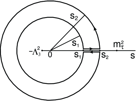
Figure 1: Contour integral

$$W(s)=(s-s_{1})(s_{2}-s)$$ (36)

The sum of integrals over cut edges is $2i~{}\int\limits^{s_{2}}_{s_{1}}~{}W(s)Im\Pi(s)ds$. This sum is equal to the sum of integrals with inverse sign over the circles, for which owing to that the weight function vanishes at the points $s_{1}$ and $s_{2}$, one may take $\Pi^{(QCD)}(s)$ instead of the true value $\Pi(s)$.

Making use of the analytical properties of $\Pi^{(QCD)}(s)$, let us transform the sum of integrals over circles into the integral from $Im\Pi^{(QCD)}(s)$ over the cut from $s_{1}$ to $s_{2}$. Finally, we obtain the following sum rule

$$\int\limits^{s_{2}}_{s_{1}}~{}W(s)Im\Pi(s)ds=\int\limits^{s_{2}}_{s_{1}}~{}W(s)Im\Pi^{(QCD)}(s)ds$$ (37)

To compare QCD predictions with experiment, let us introduce the notations

$$U_{B}=\int\limits^{s_{2}}_{s_{1}}~{}W(s)Im\Pi_{B}(s)ds/\int\limits^{s_{2}}_{s_{1}}~{}W(s)Im\Pi^{(QCD)}_{B}(s)ds$$ (38)

where $B=V,A,~{}V+A$. The results of the calculations of $U_{B}$ are given in Table 1.

Table 1.

Comparison of the sum rules (37) with the ALEPH experiment.

$U_{B}$ is given by Eq.(38). $Im\Pi_{B}(s)$ is obtained from the ALEPH experimental data. $Im\Pi^{(QCD)}_{B}(s)$ is calculated by three-loop approximation of QCD at $\Lambda_{3}=618MeV$. $s_{1}$, $s_{2}$ are given in $GeV^{2}$.

$s_{2}$	1.2	1.4	1.6	1.8	2	2.2	2.4	2.6	2.8	3
$U_{V}$	0.552	0.489	0.479	0.498	0.534	0.592	0.668	0.745	0.816	0.881
$U_{A}$	1.169	1.398	1.502	1.514	1.465	1.389	1.309	1.229	1.161	1.107	$s_{1}=0.8$
$U_{V+A}$	0.861	0.942	0.988	1.003	0.995	0.985	0.982	0.981	0.982	0.984
$s_{2}$	1.2	1.4	1.6	1.8	2	2.2	2.4	2.6	2.8	3
$u_{V}$	0.438	0.425	0.451	0.494	0.546	0.62	0.71	0.796	0.871	0.939
$u_{A}$	1.491	1.629	1.649	1.594	1.493	1.383	1.279	1.889	1.114	1.059	$s_{1}=1$
$u_{V+A}$	0.967	1.024	1.047	1.039	1.015	0.995	0.998	0.986	0.986	0.988
$s_{2}$	1.4	1.6	1.8	2	2.2	2.4	2.6	2.8	3
$u_{V}$	0.429	0.477	0.531	0.592	0.677	0.778	0.869	0. 945	1.011
$u_{A}$	1.712	1.668	1.563	1.427	1.299	1.188	1.098	1.027	0.978	$s_{1}=1.2$
$u_{V+A}$	1.065	1.069	1.042	1.003	0.98	0.976	0.976	0.979	0.983
$s_{2}$	1.6	1.8	2	2.2	2.4	2.6	2.8	3
$u_{V}$	0.533	0.586	0.65	0.749	0.862	0.956	1.028	1.091
$u_{A}$	1.601	1.456	1.302	1.172	1.067	0.986	0.927	0.891	$s_{1}=1.4$
$u_{V+A}$	1.063	1.015	0.968	0.951	0.956	0.963	0.970	0.978
$s_{2}$	1.8	2	2.2	2.4	2.6	2.8	3
$u_{V}$	0.642	0.715	0.837	0.962	1.053	1.118	1.173
$u_{A}$	1.299	1.146	1.032	0.944	0.88	0.833	0.816	$s_{1}=1.6$
$u_{V+A}$	0.964	0.922	0.924	0.944	0.959	0.97	0.98
$s_{2}$	2	2.2	2.4.	2.6	2.8	3
$u_{V}$	0.788	0.956	1.086	1.161	1.209	1.252
$u_{A}$	1.006	0.918	0.847	0.799	0.77	0.765	$s_{1}=1.8$
$u_{V+A}$	0.884	0.923	0.958	0.974	0.983	0.922
$s_{2}$	2.2	2.4	2.6	2.8	3
$u_{V}$	1.133	1.217	1.255	1.281	1.312
$u_{A}$	0.833	0.778	0.744	0.728	0.738	$s_{1}=2$
$u_{V+A}$	0.972	0.993	0.996	0.998	1.005

It is seen from Table 1 that QCD predictions agree with experiment for $V+A$ and disagree with experiments for $V$ and $A$ separately. The results do not change if one takes the weight function of the form $(s-s_{1})^{n}(s_{2}-s)^{n}$, $n=2,3,...10$.

Let us consider $V-A$. In this case $Im(\Pi^{(QCD)}_{V}(s)-\Pi^{(QCD)}_{A}(s))=0$,   while $Im(\Pi_{V}(s)-\Pi_{A}(s))\not=0$. Try to eliminate this disagreement with the help of instantons.

The instanton contribution into $\Pi^{(1)}_{V}(s)-\Pi^{(1)}_{A}(s)$ in the model considered in [3] is given by the formula (39) [3]:

$$\Pi^{(1)}_{V,inst.}(s)-\Pi^{(1)}_{A,inst}(s)=\int\limits^{\infty}_{0}d\rho n(\rho)\Biggl{[}-\frac{4}{s^{2}}-\frac{4\rho^{2}}{s}~{}K^{2}_{1}(\rho\sqrt{-s})\Biggr{]}$$ (39)

$K_{1}$ is the Macdonald function. Introduce the notations

$$L_{Exp}=\int\limits^{s_{2}}_{s_{1}}~{}W(s)Im(\Pi^{(1)}_{V}(s)-\Pi^{(1)}_{A}(s))ds$$ (40)

$$L_{inst}=\int\limits^{s_{2}}_{s_{1}}~{}W(s)Im(\Pi^{(1)}_{V,inst}(s)-\Pi^{(1)}_{A,inst}(s))ds$$ (41)

The results of $L_{Exp}$ and $L_{inst}$ calculations are given in Table 2 for $n(\rho)=n_{0}\delta(\rho-\rho_{0})$ $\rho_{0}=1.7GeV^{-1}$,  $n_{0}=1.5\cdot 10^{-3}GeV^{4}$.

Table 2. $s_{1}=0.8GeV^{2}$.

$s_{2}/GeV^{2}$	1	1.2	1.4	1.6	1.8
$L_{Exp}$	-0.00042	-0.022	-0.107	-0.286	-0.554
$L_{inst}$	0.000144	0.00089	0.00234	0.00427	0.00634
$L_{Exp}/L_{inst}$	-2.907	-24.147	-45.8	-66.82	-87.34

$s_{2}/GeV^{2}$	2	2.2	2.4	2.6	2.8	3
$L_{Exp}$	-0.878	-1.198	-1.442	-1.572	-1.563	-1.402
$L_{inst}$	0.00815	0.00933	0.00955	0.00853	0.00619	0.00209
$L_{Exp}/L_{inst}$	-107.7	-128.7	-151.1	-184.2	-256.7	-670.7

It is seen from Table 2 that instantons (in the model under consideration) cannot eliminate the disagreement between QCD theory and experiment.

5 NEW QCD PARAMETERS AND ELIMINATION
OF CONTRADICTIONS

In my opinion, the only possible way to resolve the discrepancy which follows from the sum rules (37) is to change the conventional value $\Lambda^{conv}_{3}\sim 600MeV$ by $\Lambda^{new}_{3}\sim 1600MeV$. Because $s_{1}$ must be larger than $\Lambda^{2}_{3}\sim 2.5GeV^{2}$, the sum rules (38) become meaningless. At $\Lambda^{new}_{3}\sim 1600MeV$ we have a possibility to fulfill the requirement of microcausality and unitarity to omit the nonphysical cut.

The contribution of the physical cut

$$R^{QCD,S=0}_{\tau,V+A}=6|V_{ud}|^{2}S_{EW}\int\limits^{m^{2}_{\tau}}_{0}~{}\frac{ds}{m^{2}_{\tau}}(1-\frac{s}{m^{2}_{\tau}})^{2}(1+\frac{2s}{m^{2}_{\tau}})(1+r(s))ds=3.483\pm 0.022$$ (42)

agrees with experiment (24) at

$$\Lambda_{3}=\Lambda^{new}_{3}=(1565\pm 193)MeV$$ (43)

The value $\Lambda^{new}_{3}$ in eq.(43) differs from $\Lambda^{new}_{3}$ in eq.(28) since in (28) we take into account the contribution of the nonphysical cut. It is my belief, that the nonphysical cut must be absent. In spite of that the nonphysical cut is a consequence of 3-loop in p QCD, if we are able to eliminate this drawback, we must do it. But at $\Lambda_{3}\sim 600MeV$ we cannot do it while at $\Lambda_{3}\sim 1600MeV$ we can. In what follows we put $\Lambda_{3}=(1565\pm 193)MeV$ and omit the nonphysical cut contribuion.

6 TRANSITIONS TO A LARGER NUMBER OF FLAVOURS

Let us introduce the notations

$$f_{n_{f}}(a)=\frac{1}{a}+b^{(n_{f})}_{1}~{}lna-\frac{1}{\sqrt{b^{(n_{f})^{2}}_{1}-4b^{(n_{f})}_{2}}}\Biggl{[}\frac{1}{x^{(n_{f})^{2}}_{1}}~{}ln(a-x^{(n_{f})}_{1})~{}-\frac{1}{x^{(n_{f})^{2}}_{2}}ln(a-x^{(n_{f})}_{2})\Biggr{]},~{}~{}n_{f}\leq 5$$ (44)

$$f_{n_{f}}(a)=\frac{1}{a}+b^{n_{f})}_{1}~{}lna-\frac{1}{\sqrt{b^{(n_{f})^{2}}-4b^{(n_{f})}_{2}}}\Biggl{[}\frac{1}{x^{(n_{f})^{2}}_{1}}~{}ln(a-x^{(n_{f})}_{1})-\frac{1}{x^{(n_{f})^{2}}}~{}ln(x^{(n_{f})}_{2}-a)\Biggr{]},~{}~{}n_{f}=6$$ (45)

where

$$x^{(n_{f})}_{1,2}=\frac{-b^{(n_{f})}_{1}\pm\sqrt{b^{(n_{f})^{2}}_{1}-4b^{(n_{f})}_{2}}}{2b^{(n_{f})}_{2}}$$ (46)

$$x^{(3)}_{1}=-0.0497+0.107i,~{}~{}x^{(3)}_{2}=x^{(3)*}_{1},~{}~{}x^{(4)}_{1}=-0.0632+0.1296i,~{}~{}x^{(4)}_{2}=x^{(4)*}_{1},$$

$$x^{(5)}_{1}=-0.107+0.176i,~{}~{}x^{(5)}_{2}=x^{(5)*}_{1},~{}~{}x^{(6)}_{1}=-0.213,~{}~{}x^{(6)}_{2}=1.013$$

The value $a(q^{2})$ is found by numerical solution of the equation

$$\beta^{(n_{f})}_{0}~{}ln\Biggl{(}-\frac{q^{2}+i0}{\Lambda^{2}_{f}}\Biggr{)}=f_{n_{f}}(a),~{}~{}q^{2}>0,~{}~{}n_{f}=3,4,5,6$$ (47)

The function $r(s)$ can be obtained with the help of Eqs.(19,12).

In the evolution upwards to larger energies the matching of $r(q^{2})$ at the masses $J/\psi$, $\Upsilon$ and $2m_{t}$ is performed.

There are three alternatives:

1) The nonphysical cut is absent $\Lambda^{new}_{3}=(1565\pm 193)MeV$. The Adler function $d(q^{2})$ may be written in the form

$$d(q^{2})=d^{(3)}(q^{2})+d^{(4)}(q^{2})+d^{(5)}(q^{2})+d^{(6)}(q^{2})$$ (48)

where

$$d^{(3)}(q^{2})=-q^{2}\int\limits^{m^{2}_{\psi}}_{0}\frac{r_{3}(q^{\prime 2})dq^{\prime 2}}{(q^{\prime 2}-q^{2})^{2}}$$ (49)

is the contribution of the part of the cut with 3 flavours into Adler function. Similarly,

$$d^{(4)}(q^{2})=-q^{2}~{}\int\limits^{m^{2}_{\Upsilon}}_{m^{2}_{\psi}}~{}\frac{r_{4}(q^{\prime 2})dq^{\prime 2}}{(q^{\prime 2}-q^{2})^{2}}$$ (50)

is the contribution of the part of the cut with 4 flavours into Adler function

$$d^{(5)}(q^{2})=-q^{2}~{}\int\limits^{4m^{2}_{t}}_{m^{2}_{\Upsilon}}~{}\frac{r_{5}(q^{\prime 2})dq^{\prime 2}}{(q^{\prime 2}-q^{2})^{2}}$$ (51)

is the contribution of the part of the cut with 5 flavours into Adler function

$$d^{(6)}(q^{2})=-q^{2}~{}\int\limits^{\infty}_{4m^{2}_{t}}~{}\frac{r_{6}(q^{\prime 2})dq^{\prime 2}}{(q^{\prime 2}-q^{2})^{2}}$$ (52)

is the contribution of the part of the cut with 6 flavours into Adler function.

The number of flavours for $r(q^{2})$ on the cut is a certain number in contrast to the number of flavours at the point of the complex plane $q^{2}$ off the cut. Let us consider $q^{2}=-m^{2}_{Z}$ and find $\alpha_{s}(-m^{2}_{Z})$.

Return to formula (13).The coefficients $d_{1}$ and $d_{2}$ in (13) are defined for a certain number of flavours.

Introduce

$$d^{(av)}_{1}(-m^{2}_{Z})=(d^{(3)}_{1}d^{(3)}(-m^{2}_{Z})+d^{(4)}_{1}d^{(4)}(-m^{2}_{Z})+d^{(5)}_{1}d^{(5)}(-m^{2}_{Z})+d^{(6)}_{1}d^{(6)}(-m^{2}_{Z}))/d(-m^{2}_{Z})$$ (53)

$$d^{(av)}_{2}(-m^{2}_{Z})=(d^{(3)}_{2}d^{(3)}(-m^{2}_{Z})+d^{(4)}_{2}d^{(4)}(-m^{2}_{Z})+d^{(5)}_{2}d^{(5)}(-m^{2}_{Z})+d^{(6)}_{2}d^{(6)}(-m^{2}_{Z}))/d(-m^{2}_{Z})$$ (54)

The values $d^{(n_{f})}(-m^{2}_{Z})$ have been calculated.

$$d^{(3)}(-m^{2}_{Z})=0.000169,~{}~{}d^{(4)}(-m^{2}_{Z})=0.000823,~{}~{}d^{(5)}(-m^{2}_{Z})=0.0432$$

$$d^{(6)}(-m^{2}_{Z})=0.00218,~{}~{}d(-m^{2}_{Z})=0.0464$$ (55)

Formula (13) is replaced by

$$d(-m^{2}_{Z})=4a(-m^{2}_{Z})(1+4d^{(av)}_{1}(-m^{2}_{Z})a(-m^{2}_{Z})+16d^{(av)}_{2}(-m^{2}_{Z})a^{2}(-m^{2}_{Z}))$$ (56)

The equation (49) can be solved for $a(-m^{2}_{Z})$

$$\alpha_{s}(-m^{2}_{Z})=4\pi~{}a(-m^{2}_{Z})=0.142\pm 0.004$$ (57)

The value $\alpha_{s}(m^{2}_{Z}+i0)$ is evaluated from (6,8).

$$\alpha_{s}(m^{2}_{Z}+i0)=0.131\pm 0.003+(0.037\pm 0.002)i$$

$$|\alpha_{s}(m^{2}_{Z}+i0)|=0.136\pm 0.004$$ (58)

In a similar way $\alpha_{s}(q^{2})$ can be calculated at arbitrary $q^{2}$. The values of $\alpha_{s}$ at the interesting points are given in Table 3.

Table 3.

The calculation of $\alpha_{s}(q^{2})$ at different $q^{2}$ in approximation of 1-4 loops. The matching of $r(q^{2})$ at the masses of $J/\psi$, $\Upsilon$ and $2m_{t}$ is performed. The contribution of nonphysical cut is omitted.

Approximation	$\Lambda_{3}/MeV$	$\Lambda_{4}/MeV$	$\Lambda_{5}/MeV$	$\Lambda_{6}/MeV$	$\alpha_{s}(0)$	$\alpha_{s}(-m^{2}_{\tau})$
One loop	$618\pm 59$	$508\pm 51$	$377\pm 40$	$191\pm 22$	1.396	$0.469\pm 0.018$
Two loops	$1192\pm 136$	$956\pm 113$	$678\pm 86$	$301\pm 42$	$0.895\pm 0.001$	$0.387\pm 0.015$
Three loops	$1565\pm 193$	$1257\pm 158$	$872\pm 119$	$312\pm 47$	$0.749\pm 0.001$	$0.379\pm 0.013$
Four loops	$1862\pm 230$	$1503\pm 189$	$1064\pm 145$	$202\pm 31$	$0.749\pm 0.001$	$0.379\pm 0.013$

Approximation	$\alpha_{s}(m^{2}_{\tau}+i0)$	$\alpha_{s}(-m^{2}_{\psi})$	$\alpha_{s}(m^{2}_{\psi}-0+i0)$
One loop	$0.356\pm 0.019+(0.306\pm 0.017)i$	$0.377\pm 0.014$	$0.276\pm 0.010+(0.216\pm 0.013)i$
Two loops	$0.355\pm 0.014+(0.270\pm 0.014)i$	$0.332\pm 0.013$	$0.265\pm 0.003+(0.200\pm 0.014)i$
Three loops	$0.365\pm 0.023+(0.264\pm 0.013)i$	$0.322\pm 0.009$	$0.272\pm 0.015\pm(0.201\pm 0.014)i$
Four loops	$0.363\pm 0.013+(0.263\pm 0.013)i$	$0.326\pm 0.012$	$0.273\pm 0.016\pm(0.202\pm 0.014)i$

Approximation	$\alpha(m^{2}_{\psi}+0+i0)$	$\alpha_{s}(-m^{2}_{\Upsilon})$	$\alpha_{s}(m^{2}_{\Upsilon}-0+i0)$
One loop	$0.291\pm 0.012+(0.206\pm 0.013)i$	$0.254\pm 0.008$	$0.206\pm 0.005+(0.107\pm 006)i$
Two loops	$0.284\pm 0.002+(0.193\pm 0.014)i$	$0.234\pm 0.009$	$0.192\pm 0.004+(0.100\pm 007)i$
Three loops	$0.293\pm 0.017+(0.199\pm 0.015)i$	$0.237\pm 0.009$	$0.194\pm 0.006+(0.106\pm 0.008)i$
Four loops	$0.294\pm 0.018+(0.199\pm 0.015)i$	$0.237\pm 0.009$	$0.194\pm 0.007+(0.104\pm 0.007)i$

Approximation	$\alpha_{s}(m^{2}_{\Upsilon}+0+i0)$	$\alpha_{s}(-m^{2}_{z})$	$\alpha_{s}(\psi m^{2}_{z}+i0)$
One loop	$0.211\pm 0.006+(0.100\pm 0.005)i$	$0.142\pm 0.003$	$0.141\pm 0.006+(0.039\pm 0.002)i$
Two loops	$0.199\pm 0.005+(0.093\pm 0.007)i$	$0.137\pm 0.002$	$0.129\pm 0.003+(0.036\pm 0.002)i$
Three loops	$0.203\pm 0.007+(0.098\pm 0.007)i$	$0.142\pm 0.004$	$0.131\pm 0.003+(0.037\pm 0.002)i$
Four loops	$0.204\pm 0.008+(0.099\pm 0.007)i$	$0.141\pm 0.004$	$0.131\pm 0.003+(0.038\pm 0.002)i$

Approximation	$r(m^{2}_{z})$	$R_{l}$
One loop	$0.0462\pm 0.0009$	$20.856\pm 0.017$
Two loops	$0.0458\pm 0.0011$	$20.848\pm 0.021$
Three loops	$0.0464\pm 0.0012$	$20.860\pm 0.023$
Four loops	$0.0465\pm 0.0012$	$20.861\pm 0.023$

2. The nonphysical cut is taken into account , $\Lambda^{new}_{3}=(1666\pm 7)MeV$. In this case the lower limit of the integral in eq.(49) is equal to $-\Lambda^{2}_{3}$ and in the three-loop approximaion $\Lambda_{4}=1591MeV$, $\Lambda_{5}=791MeV$, $\Lambda_{6}=280MeV$. Errors in this case are very small. The results of the calculations in the three-loop approximation are the following:

$$\alpha_{s}(-m^{2}_{\tau})=1.575,~{}~{}\alpha_{s}(m^{2}_{\tau}+i0)=0.142+0.272i,~{}~{}\alpha_{s}(-m^{2}_{\psi})=0.484$$

$$\alpha_{s}(m^{2}_{\psi}-0+i0)=0.179+0.209i~{}~{}\alpha_{s}(m^{2}_{\psi}+0+0i)=0.223+229i,~{}~{}\alpha_{s}(-m^{2}_{\Upsilon})=0.253$$

$$\alpha_{s}(m^{2}_{\Upsilon}-0+i0)=0.202+0.110i,~{}~{}\alpha_{s}(m^{2}_{\Upsilon}+0+0i)=0.189+0.093i,~{}~{}\alpha_{s}(-m^{2}_{z})=0.139$$ (59)

$$\alpha_{s}(-m^{2}_{z}+i0)=0.129+0.036i,~{}~{}r(m^{2}_{z})=0.0457,~{}~{}R_{l}=20.845$$

3. The nonphysical cut is taken into account, $\Lambda^{conv.}_{3}=(618\pm 29)MeV$. The results of the calculations in 1-4 loop approximaion are given in Table 4.

Table 4.

The calculation of $\alpha_{s}(q^{2})$ at different $q^{2}$ in 1-4 loop approximation. The matching of $r(q^{2})$ at the masses of $J/\psi$, $\Upsilon$ mesons and of $2m_{\tau}$ is performed. The contribution of nonphysical cut is taken into acccount.

Approx.	$\Lambda_{3}/MeV$	$\Lambda_{4}/MeV$	$\Lambda_{5}/MeV$	$\Lambda_{6}/MeV$	$\alpha_{s}(-m^{2}_{\tau})$	$\alpha_{s}(m^{2}_{\tau}+i0)$
One loop	$370\pm 19$	$296\pm 16$	$211\pm 13$	$102\pm 7$	$0.445\pm 0.015$	0.$222+(0.222\pm 007)i$
Two loops	$539\pm 25$	$416\pm 21$	$275\pm 15$	$111\pm 7$	$0.371\pm 0.012$	$0.19+(0.174\pm 0.006)i$
Three loops	$618\pm 29$	$475\pm 24$	$301\pm 16$	$96\pm 5$	$0.354\pm 0.010$	$0.186\pm 0.001+(0.162\pm 0.005)i$
Four loops	$720\pm 33$	$557\pm 28$	$359\pm 20$	$61\pm 4$	$0.375\pm 0.012$	$0.184\pm 0.001+(0.161\pm 0.005)i$

Approx.	$\alpha_{s}(-m^{2}_{\psi})$	$\alpha_{s}(m^{2}_{\psi}-0+i0)$	$\alpha_{s}(m^{2}_{\psi}+0+i0)$
One loop	$0.33\pm 0.01$	$0.212\pm 0.002+(0157\pm 0.005)i$	$0.222\pm 0.002+(0.148\pm 0.005)i$
Two loops	$0.277\pm 0.006$	$0.182\pm 0.002+(0.125\pm 0.004)i$	$0.192\pm 0.002+(0.118\pm 0.004)i$
Three loops	$0.266\pm 0.006$	$0.177\pm 0.001+(0.116\pm 0.004)i$	$0.187\pm 0.002+(0.112\pm 0.003)i$
Four loops	$0.273\pm 0.006$	$0.177\pm 0.001+(0.116\pm 0.003)i$	$0.187\pm 0.002\pm(0.111\pm 0.003)i$

Approx.	$\alpha_{s}(-m^{2}_{\Upsilon})$	$\alpha_{s}(m^{2}_{\Upsilon}-0+i0)$	$\alpha_{s}(m^{2}_{\Upsilon}+0+i0)$
One loop	$0.180\pm 0.003$	$0.180\pm 0.002+(0.082\pm 0.002)i$	$0.184\pm 0.002+(0.076\pm 0.002)i$
Two loops	$0.189\pm 0.003$	$0.157\pm 0.002+(0.066\pm 0.002)i$	$0.161\pm 0.002+(0.061\pm 0.002)i$
Three loops	$0.184\pm 0.003$	$0.154\pm 0.002+(0.063\pm 0.002)i$	$0.159\pm 0.002+(0.059\pm 0.001)i$
Four loops	$0.185\pm 0.003$	$0.154\pm 0.002\pm(0.063\pm 0.002)i$	$0.159\pm 0.002+(0.059\pm 0.002)i$

Approx.	$\alpha_{s}(-m^{2}_{z})$	$\alpha_{s}(m^{2}_{z}+i0)$	$r(m^{2}_{z})$	$R_{l}$
One loop	$0.135\pm 0.001$	$0.186\pm 0.002+(0.032\pm 0.001)i$	$0.0420\pm 0.0004$	$20.772\pm 0.008$
Two loops	$0.120\pm 0.001$	$0.113\pm 0.001+(0.0274\pm 0.0005)i$	$0.0395\pm 0.0003$	$20.721\pm 0.007$
Three loops	$0.118\pm 0.001$	$0.112\pm 0.001+(0.0267\pm 0.0004)i$	$0.0389\pm 0.0003$	$20.710\pm 0.007$
Four loops	$0.118\pm 0.001$	$0.111\pm 0.001+(0.0266\pm 0.004)i$	$0.0388\pm 0.0003$	$20.708\pm 0.007$

Unlike conventional matching procedure at negative $q^{2}$, the matching of $r(q^{2})$ on the masses of $J/\Psi$, $\Upsilon$ mesons and of $2m_{t}$ is performed. The value $\alpha_{s}(-m^{2}_{z})$ is practically independent of the matching procedure. I believe, that the first alternative is the best.

7 Comparison of the calculated values $R_{T}(s)$ with the measured values $R_{E}(s)$.

The value $R_{T}(s)$ is calculated by the formula

$$R_{T}(s)=3~{}\sum~{}e^{2}_{q}(1+r(s))$$ (60)

The results of the calculations of $R(s)$ in three loop-approximation and of their comparison with experiments are given in Table 5 for $2\leq\sqrt{s}\ll 4.8GeV$ and for $12\leq\sqrt{s}\leq 46.6~{}GeV$ in Table 6. The calculated values of the function $R(s)$ are in an excellent agreement with the experiment except for the resonance region $3.7\leq\sqrt{s}\leq 4.4~{}GeV$. But the accuracy of measurements of $R(s)$ is insufficient to define the value $r(s)$ with a good accuracy.

Table 5

Comparison of the calculated values $R_{T}(s)$ with the measured values $R_{E}$ [21]

$E_{cm}$ (GeV)	$R_{T}$	$R_{E}$	$E_{cm}$(GeV)	$R_{T}$	$R_{E}$
2.000	2.29	$2.18.\pm 0,07\pm 0.18$	4.033	3.70	$4.32\pm 0.17\pm 0.22$
2.200	2.28	$2.38\pm 0.07\pm 0.17$	4.040	3.70	$4.40\pm 0.17\pm 0.19$
2.400	2.27	$2.38\pm 0.07\pm 0.14$	4.050	3.70	$4.23\pm 0.17\pm 0.22$
2.500	2.27	$2.39\pm 0.08\pm 0.15$	4.060	3.70	$4.65\pm 0.19\pm 0.19$
2.600	2.26	$2.38\pm 0.06\pm 0.15$	4.070	3.70	$4.14\pm 0.20\pm 0.19$
2.700	2.26	$2.30\pm 0.07\pm 0.13$	4.080	3.70	$4.24\pm 0.21\pm 0.18$
2.800	2.25	$2.27\pm 0.06\pm 0.14$	4.090	3.69	$4.06\pm 0.17\pm 0.18$
2.900	2.25	$2.22\pm 0.07\pm 0.13$	4.100	3.69	$3.97\pm 0.16\pm 0.18$
3.000	2.25	$2.21\pm 0.05\pm 0.11$	4.110	3.69	$3.92\pm 0.16\pm 0.19$
3.700	3.71	$2.23\pm 0.08\pm 0.08$	4.120	3.69	$4.11\pm 0.24\pm 0.23$
3.730	3.71	$2.10\pm 0.08\pm 0.14$	4.130	3.69	$3.99\pm 0.15\pm 0.17$
3.750	3.71	$2.47\pm 0.09\pm 0.12$	4.140	3.69	$3.83\pm 0.15\pm 0.18$
3.760	3.71	$2.77\pm 0.11\pm 0.13$	4.150	3.69	$4.21\pm 0.18\pm 0.19$
3.764	3.71	$3.29\pm 0.27\pm 0.29$	4.160	3.69	$4.12\pm 0.15\pm 0.16$
3.768	3.71	$3.80\pm 0.33\pm 0.25$	4.170	3.69	$4.12\pm 0.15\pm 0.19$
3.770	3.71	$3.55\pm 0.14\pm 0.19$	4.180	3.69	$4.18\pm 0.17\pm 0.18$
3.772	3.71	$3.12\pm 0.24\pm 0.23$	4.190	3.69	$4.01\pm 0.14\pm 0.14$
3.776	3.71	$3.26\pm 0.26\pm 0.19$	4.200	3.69	$3.87\pm 0.16\pm 0.16$
3.780	3.71	$3.28\pm 0.12\pm 0.12$	4.210	3.69	$3.20\pm 0.16\pm 0.17$
3.790	3.71	$2.62\pm 0.11\pm 0.10$	4.220	3.69	$3.62\pm 0.15\pm 0.20$
3.810	3.71	$2.38\pm 0.10\pm 0.12$	4.230	3.69	$3.21\pm 0.13\pm 0.15$
3.850	3.70	$2.47\pm 0.11\pm 0.13$	4.240	3.69	$3.24\pm 0.12\pm 0.15$
3.890	3.70	$2.64\pm 0.11\pm 0.15$	4.245	3.69	$2.97\pm 0.11\pm 0.14$
3.930	3.70	$3.18\pm 0.14\pm 0.17$	4.250	3.69	$2.71\pm 0.12\pm 0.13$
3.940	3.70	$2.94\pm 0.13\pm 0.19$	4.255	3.69	$2.88\pm 0.11\pm 0.14$
3.950	3.70	$2.97\pm 0.13\pm 0.17$	4.260	3.69	$2.97\pm 0.11\pm 0.14$
3.960	3.70	$2.79\pm 0.12\pm 0.17$	4.265	3.69	$3.04\pm 0.13\pm 0.14$
3.970	3.70	$3.29\pm 0.13\pm 0.13$	4.270	3.69	$3.26\pm 0.12\pm 0.17$
3.980	3.70	$3.13\pm 0.14\pm 0.16$	4.280	3.69	$3.08\pm 0.12\pm 0.15$
3.990	3.70	$3.06\pm 0.15\pm 0.18$	4.300	3.69	$3.11\pm 0.12\pm 0.12$
4.000	3.70	$3.16\pm 0.14\pm 0.15$	4.320	3.69	$2.96\pm 0.12\pm 0.14$
4.010	3.70	$3.53\pm 0.16\pm 0.20$	4.340	3.69	$3.27\pm 0.15\pm 0.18$
4.020	3.70	$4.43\pm 0.16\pm 0.21$	4.350	3.69	$3.49\pm 0.14\pm 0.14$
4.027	3.70	$4.58\pm 0.18\pm 0.21$	4.360	3.68	$3.47\pm 0.13\pm 0.18$
4.030	3.70	$4.58\pm 0.20\pm 0.23$	4.380	3.68	$3.50\pm 0.15\pm 0.17$

Table 5.   Continuation

$E_{cm}$ (GeV)	$R_{T}$	$R_{E}$
4.390	3.68	$3.48\pm 0.16\pm 0.16$
4.400	3.68	$3.91\pm 0.16\pm 0.19$
4.410	3.68	$3.79\pm 0.15\pm 0.20$
4.420	3.68	$3.68\pm 0.14\pm 0.17$
4.430	3.68	$4.02\pm 0.16\pm 0.20$
4.440	3.68	$3.85\pm 0.17\pm 0.17$
4.450	3.68	$3.75\pm 0.15\pm 0.17$
4.460	3.68	$3.66\pm 0.17\pm 0.16$
4.480	3.68	$3.54\pm 0.17\pm 0.18$
4.500	3.68	$3.49\pm 0.14\pm 0.15$
4.520	3.68	$3.25\pm 0.13\pm 0.15$
4.540	3.68	$3.23\pm 0.14\pm 0.18$
4.560	3.68	$3.62\pm 0.13\pm 0.16$
4.60	3.68	$3.31\pm 0.11\pm 0.16$
4.80	3.67	$3.66\pm 0.14\pm 0.19$

Table 6.

Comparison of the calculated values $R_{T}(s)$ with the measured values $R_{E}$ [22-24]

$s/Gev$	$R_{T}$	$R_{E}$	$\sqrt{s}/GeV$
		[22]
14.0	3.92	$4.10\pm 0.11\pm 0.11$	29.93	3.88	$3.55\pm 0.40\pm 0.11$
22.0	3.89	$3.86\pm 0.12\pm 0.11$	30.38	3.87	$3.85\pm 0.19\pm 0.12$
33.8	3.87	$3.74\pm 0.10\pm 0.10$	31.29	3.87	$3.83\pm 0.28\pm 0.11$
38.3	3.86	$3.89\pm 0.10\pm 0.09$	33.89	3.87	$4.16\pm 0.10\pm 0.12$
41.5	3.86	$4.03\pm 0.17\pm 0.10$	34.50	3.87	$3.93\pm 0.20\pm 0.12$
43.5	3.86	$3.97\pm 0.08\pm 0.09$	35.01	3.87	$3.93\pm 0.10\pm 0.12$
44.2	3.86	$4.01\pm 0.10\pm 0.08$	34.45	3.87	$3.93\pm 0.18\pm 0.12$
46.0	3.86	$4.09\pm 0.21\pm 0.10$	36.38	3.87	$3.71\pm 0.21\pm 0.11$
46.6	3.86	$4.20\pm 0.36\pm 0.10$	40.32	3.86	$4.05\pm 0.19\pm 0.14$
		[23]	41.18	3.86	$4.21\pm 0.22\pm 0.14$
29	3.88	$3.96\pm 0.09$	42.55	3.86	$4.20\pm 0.22\pm 0.14$
		[24]	43.53	3.86	$4.00\pm 0.20\pm 0.14$
12	3.93	$3.45\pm 0.27\pm 0.13$	44.41	3.86	$3.98\pm 0.20\pm 0.14$
14.04	3.92	$3.94\pm 0.14\pm 0.14$	45.59	3.86	$4.40\pm 0.22\pm 0.15$
22	3.89	$4.11\pm 0.13\pm 0.12$	46.47	3.86	$4.04\pm 0.24\pm 0.14$
25.01	3.88	$4.24\pm 0.29\pm 0.13$
27.66	3.88	$3.85\pm 0.48\pm 0.12$

8 COMPARISON WITH $\alpha_{s}(s)$ OBTAINED FROM THE SUM RULES

Perturbative corrections to two measurements, namely, the Gross-Llewellyn Smith sum rule [7] for the deep inelastic neutrino scattering and the Bjorken sum rule [8] for polarized structure functions, have been determined:

$$\alpha_{s}(-3GeV^{2})=0.28\pm 0.035(stat)\pm 0.050(sys.)~{}[12,25]$$ (61)

and

$$\alpha_{s}(-2.5GeV^{2})=0.375^{+0.062}_{-0.081}~{}[12,26-28]$$ (62)

The results of the calculations give

$$\alpha_{s}(-3GeV^{2})=0.381\pm 0.013$$ (63)

$$\alpha_{s}(-2.5GeV^{2})=0.39\pm 0.013$$ (64)

9 Calculation of $R_{l}$

The value $R_{l}=\Gamma(Z\to hadrons)/\Gamma(Z\to leptons)$ is parametrized by the latest version of ZFITTER [29]

$$R_{l}=19.934\Biggl{(}1+1.045(\frac{\alpha_{s}}{\pi})+0.94(\frac{\alpha_{s}}{\pi})^{2}-15(\frac{\alpha_{s}}{\pi})^{3}\Biggr{)}$$ (65)

This is the conventional method. In this parametrization

$$M_{H}=300GeV,~{}~{}M_{t}=174.1GeV,~{}~{}0.1<\alpha_{s}<0.13.$$

In the method under investigation Eq.(65 ) should be changed by the formula

$$R_{l}=19.934(1+r(m^{2}_{Z}))$$ (66)

The calculated values of $r(m^{2}_{z})$ and of $R_{l}$ are presented in Tables 3,4 in 1-4 loop approximation. The value $R_{l}$ can be compared with the measurement [12].

$$\Gamma(Z\to hadrons)=(1744.4\pm 2)~{}MeV$$ (67)

$$\Gamma(Z\to leptons)=(83.984\pm 0.086)~{}MeV$$ (68)

and

$$R_{l}=20.771\pm 0.045$$ (69)

The value $R_{l}$ (69) does not contradict $R_{l}$ from Tables 3,4.

10 On analiticity of $\alpha_{s}(q^{2})$

In the interesting papers [30] the renormgroup was combined with analiticity of $\alpha_{s}(q^{2})$. It was assumed that $\alpha_{s}(q^{2})$ is an analytic function of $q^{2}$ in the whole complex $q^{2}$ plane with a cut along the poitive $q^{2}$ semiaxis. In particular, it was obtained that $\alpha_{s}(0)$ is universal and independent of the number of loops, $\Lambda_{3}$ and

$$\alpha_{s}(0)=4\pi/\beta^{(3)}_{0}=1.396$$ (70)

The analogous formula had been also obtained in paper [1]. As is seen from Table 3, eq.(70) is valid only in one-loop approximation.

If $\alpha_{s}(q^{2})$ has correct analiticity, the Adler function will have correct analiticity too, but a reverse statement is invalid. If Adler function has correct analiticity, function $a(q^{2})$ may have, generally speaking, additional singularities. This statement will be evident, if one considers eq.(13) as an equation relative to $a(q^{2})$. If only eq.(13) is solved by expansion in $a(q^{2})$, analiticity $a(q^{2})$ will be the same as the Adler function. However, using of $d(q^{2})$ expansion in $a(q^{2})$ at small $q^{2}$ seems to be doubtful.

11 Conclusion.

Concluding, let us formulate the main results of this paper.

1) There are two and only two values of $\Lambda_{3}$, at which $R_{\tau,V+A}=3.475\pm 0.022$, one conventional value $\Lambda^{conv}_{3}=(618\pm 29)~{}MeV$ ($\Lambda_{3}$ is defined by eq.(7)) and the other, found in this paper, $\Lambda^{new}_{3}=(1666\pm 7)~{}MeV$.

2. The renormgroup calculation leads to appearance of a nonphysical cut in the Adler function. In complete theory, where everything is taken into account, the nonphysical cut must be absent. The question arises, if it is possible to neglect nonphysical cut at the present situation with the theory. At conventional value $\Lambda_{3}=\Lambda^{conv}_{3}$ it is impossible. The new value, $\Lambda_{3}=\Lambda^{new}_{3}$ is more preferable than $\Lambda_{3}=\Lambda^{conv}_{3}$, since at $\Lambda_{3}=\Lambda^{new}_{3}$ the contribution of nonphysical cut into $R_{\tau,V+A}$ is practically absent.

3) At $\Lambda_{3}=\Lambda^{conv}_{3}$ there is an essential disagreement between the ALEPH experiment and new obtained sum rules, which follow only from analytical properties of the polarization operator. This disagreement disappears if $\Lambda_{3}=\Lambda^{new}_{3}$.

4) In 1-4 loop approximation all calulations are made exactly, without $\pi/ln\frac{Q^{2}}{\Lambda^{2}}$ expansion.

5) At $\Lambda^{new}_{3}=(1565\pm 193)~{}MeV$ the nonphysical cut may be omitted, the polarization operator has correct analytical properties and $R_{\tau,V+A}=3.475\pm 0.022$. But in this case QCD parameters essentially differ from conventional values.

Acknowledgements

In conclusion, thanks are due to B.L.Ioffe and K.N.Zyablyuk for useful discussions and to K.N.Zyablyuk for checking the correctness of tables 1,2. The author is also indebted to M.Davier for his kind presentation of the ALEPH experimental data.

References

- [1] B.V.Geshkenbein and B.L.Ioffe, Pis’ma Zh.Eksp.Teor.Fis. 70, 167 (1999).
- [2] B.L.Ioffe and K.N.Zyablyuk, Nucl.Phys. A687, 437 (2001).
- [3] B.V.Geshkenbein, B.L.Ioffe and K.N.Zyablyuk, Phys.Rev. D64, 093009 (2001)
- [4] ALEPH Collaboration, R.Barate et al. Eur.Phys.J. 4, 409 (1998). The data files are taken from http://alephwww.cern.ch/ALPUB/paper/paper.html.
- [5] OPAL Collaboration K.Ackerstaff et al. Eur.Phys.J. C 7, 571 (1999); G.Abbiend et al., ibid/ 13, 197 (2000).
- [6] CLEO Collaboraion S.J.Richichi et al., Phys.Rev. D 60, 112 002 (1999).
- [7] D.Gross and C.Llewellyn Smith, Nucl.Phys B14, 337 (1969)
- [8] J.Bjorken, Phys.Rev. D1 (1970) 1376.
- [9] O.V.Tarasov, A.A.Vladimirov and A.Ya.Zahrkov, Phys.Lett. 93B, 429 (1980); S.A.Larin and J.A.M.Vermaseren, Phys.Lett.B 303, 334 (1993).
- [10] T.van Ritberger, J.A.M.Vermaseren and S.A.Larin, Phys.Lett. B 400, 379 (1997).
- [11] K.G.Chetyrkin, A.L.Kataev and F.V.Tkachov, Phys.Lett. 85B, 277 (1979); M.Dine and J.Sapirshtein, Phys.Rev.Lett. 43, 668 (1979); W.Celmaster and R.Gonsalves, ibid 44, 560 (1988).
- [12] Particle Data Group, C.Grab et al. Phys.Rev. D66, 1 (2002).
- [13] W.J.Marciano and Sirlin, Phys.Rev.Lett 61, 1815 (1988); 56, 22 (1986).
- [14] ALEPH Collaboration, R.Barate et al., Eur.Phys.J. C11, 599 (1999).
- [15] OPAL Collaboration, G.Abbiendi et al., Eur.Phys.J. C19, 653 (2001).
- [16] E.Braaten, Phys.Rev.Lett. 60, 1606 (1988); Phys.Rev. D 39, 1458 (1989).
- [17] S.Narison and A.Pich, Phys.Lett. B211, 183 (1988).
- [18] E.Braaten, S.Narison and A.Pich, Nucl.Phys. B 373, 581 (1992).
- [19] F.Le Diberder and A.Pich, Phys.Lett. B286, 147 (1992).
- [20] M.A.Shifman, A.I.Vainstein and V.I.Zakharov, Nucl.Phys. 147, 385 (1979).
- [21] J.L.Bai et al., (Bas Collab), hep-ex 0102003.
- [22] H.J.Behrend et al., [Cello Collaboration] Phys.Lett. B183, 400 (1987).
- [23] E.Fernandes et al., [SLAC-PEP-006, MAC Collaboration], Phys.Rev. D31, 1537 (1985).
- [24] B.Naroska, [DESY-PETRA, JADE Collaboration], Phys.Rep. 148 67 (1987).
- [25] J.H.Kim et al., [CCFR Collaboration], Phys.Rev.Lett. 81, 3595 (1998).
- [26] J.Ellis and M.Karliner, Phys.Lett, B341, 397 (1995).
- [27] D.Adams et al., Phys.Lett. B329, 399 (1994).
- [28] R.Arnold et al., [E143 COllaboration], Conf on intersections of Particle and Nuclear Physics, St.Petersburg Florida, June 1994; Phys.Rev.Lett. 74, 346 (1995).
- [29] E.Tournefier, Proc. of the Quarks 98 Int.Seminar, Suzdal, Russia, May 1998; hep-ex/9810042.
-
[30]
D.V.Shirkov and I.L.Solovtsov, Phys.Rev.Let. 79, 1209
(1997);
I.L.Solovtsov and D.V.Shirkov, Phys. Lett. B442, 344 (2998);
K.A.Milton and O.P.Solovtsova, Phys.Rev. D57, 5402 (1998);
K.A.Milton, I.L.Solovtsov, and O.P.Solovtsova, ibid. 60, 016001 (1999);
A.V.Nesterenko, hep-ph/0102124; hep-ph/0102203. D.V.Shirkov, Theor.Math.Phys. 119, 55 (1999);
I.L.Solovtsov and D.V.Shirkov, Theor.Math.Phys. 120, 482 (1999);
K.A.Milton, I.L.Solovtsov and O.P.Solovtsova, Phys.Lett. B415, 104 (1997);
K.A.Milton, I.L.Solovtsov and V.I.Yasnov, hep-ph/9802282.