Abstract

Extending previous works on the spectrum of QCD₂, we now investigate the 2D analogue of meson-baryon scattering. We use semi-classical methods, perturbing around classical soliton solutions. We start with the abelian case, corresponding to one flavor, and find that in this case the effective potential is reflectionless. We obtain an explicit expression for the forward phase shift. In the non-Abelian case of several flavors, the method yields a potential which depends on the momentum of the incoming particle. In this case there is both transmission and reflection. In both cases no resonances appear. As a byproduct, we derive the general conditions for a 2D scalar quantum field theoretical action to yield a reflectionless effective potential when one expands in small fluctuations about the classical solution.

Introduction

The semi-classical approximation has been an important tool in Quantum Field Theory for some time now [1].

Typically one first finds a classical solution of the field equations, yielding some topologically stable object (an instanton, a monopole, a soliton, etc.) which cannot be reached by perturbation theory [2].

One then computes quantum fluctuations around such a soliton, yielding the quantum eigenstates, as well as the scattering matrix for interaction of the fluctuating fields with the soliton.

In the context of QCD this procedure has been applied to the Skyrme model [3], which is the same universality class as the infrared limit of large-$N_{c}$ QCD [4]. The quantum eigenstates have been obtained and interpreted as physical baryons in Ref. [5] and the corresponding $S$-matrix describing meson-baryon scattering was computed in Refs. [6]-[8] and in [9].

Still, one has to keep in mind that for QCD in 3+1 dimensions the exact low energy action is not known, so one is forced to use symmetry properties and models to construct an approximate low energy effective action which admits soliton solutions. The Skyrme model is just one specific representative of a large class of models of this kind. The large-$N_{c}$ approximation is an important guiding principle [4] for constructing such actions, but even after it is implemented, much unknown remains.

In contrast, in 1+1 dimensions it is often possible to obtain analytic solutions. Thus instead of studying an approximate effective action in 3+1 dimensions, one can analyze the exact effective action in 1+1 dimensions. The limitations of such an approach are obvious. The most striking one for QCD is the very different nature of chiral symmetry in 1+1 vs. 3+1 dimensions. Yet, for many purposes it is useful to have a strong analytic grip on the 1+1 dimensional analogues of the problems in 3+1 dimensions.

This line of thought has been pioneered by ’t Hooft [10] in his work on QCD₂ mesons in the large-$N_{c}$ limit. A lot of further progress in the study of QCD₂ was made possible through non-abelian bosonization and semiclassical methods applied to the bosonized action.

Thus the baryon spectrum of QCD₂ for general $N_{f}$ and $N_{c}$ was computed in Refs. [11],[12]; the $\bar{q}q$ content of baryons was calculated in Ref. [13] and the physical picture of baryons composed of constituent quark solitons was obtained in Ref. [14].

In this paper we will compute the meson-baryon scattering in QCD₂ at strong coupling, following the techniques of [6] applied to the bosonized action [15].

We first review the general method in Section 1, pointing out a particularly simple way of parametrizing the small fluctuations around the classical soliton.

In Sec. 2 we then work out the abelian case of one flavor at strong coupling, as a “warm-up”. It turns out that the resulting effective potential for small fluctuations is of a special kind, with no reflection. Thus the modulus of the transmission coefficient is 1, and the scattering is fully characterized by the phase shift. We compute the phase shift, which changes smoothly from $\pi$ at the threshold to 0 at infinite energy.

Motivated by the emergence of the reflectionless potential for this case, we obtain in Sec. 3 the general condition for actions leading to reflectionless effective potentials. In particular, we also find that $(\phi^{2}-a^{2})^{2}$ belongs to this category, in addition to sine-Gordon action which appears in the strong-coupling limit for one flavor.

Moving on to many flavors in Sec. 4, we find a relativistic analogue of a velocity-dependent potential, i.e. an effective potential which depends on the energy of the projectile.

In Sec. 5 we compute the energy dependence of the transmission and reflection amplitudes as well as the phase shift. The latter is ${-}{\pi\over 2}$ at the threshold, and ${-}\pi$ at infinity, with a minimum at an energy of about 1.2 times the mass of the projectile. We find no evidence for resonances.

1 General Formulation

QCD in 1+1 dimensions, bosonized in the scheme

$${[\,\,\underbrace{SU(N_{c})\vrule height=0.0pt,depth=3.01385pt,width=0.0pt}\,\,]_{\lower 3.5pt\hbox{$N_{F}$}}\atop\kern-13.99995pth}{\times\atop\phantom{A}}{[\,\,\underbrace{U(N_{F})\vrule height=0.0pt,depth=3.01385pt,width=0.0pt}\,\,]_{\lower 3.5pt\hbox{$N_{c}$}}\atop\kern-13.99995ptg}$$ (1)

is [15]

$$S[g,h,A_{+}A_{-}] = N_{c}S[g]+N_{f}S[h]$$

$$+ {N_{F}\over 2\pi}\int d^{2}x\,\hbox{Tr}_{c}\left[i\left(A_{+}h\partial_{-}h^{\dagger}+A_{-}h^{\dagger}\partial_{+}h\right)-\left(A_{+}hA_{-}h^{\dagger}-A_{-}A_{+}\right)\right]$$

(2)

$$- {1\over 2e_{c}^{2}}\int d^{2}x\,\hbox{Tr}_{c}\,F_{\mu\nu}F^{\mu\nu}+{m^{\prime}}^{2}N_{\widetilde{m}}\int d^{2}x\,\hbox{Tr}\left(g\,h+h^{\dagger}\,g^{\dagger}\right)$$

$${m^{\prime}}^{2}=m_{q}\,C\,\widetilde{m}$$

where $\widetilde{m}$ is to be fixed, $C=e^{\gamma}\approx 0.891$, and

$$S[u]\equiv S_{WZW}[u] = {1\over 8\pi}\int d^{2}x\,\hbox{Tr}\left(\partial_{\mu}u\partial^{\mu}u^{\dagger}\right)$$

(3)

$$+ {1\over 12\pi}\int_{B}d^{3}y\,\epsilon_{ijk}\,\hbox{Tr}\left[\left(u^{-1}\partial_{i}u\right)\,\left(u^{-1}\partial_{j}u\right)\,\left(u^{-1}\partial_{k}u\right)\right]$$

In the strong coupling limit ${e_{c}/m_{q}}\to\infty$ [15],

$$S_{\kern-0.70004pt\hbox{\small\it eff}} = N_{c}S[g]+m^{2}N_{m}\int d^{2}x\left(\,\hbox{Tr}\,g+\,\hbox{Tr}\,g^{\dagger}\right)$$

$$m = \left[N_{c}Cm_{q}\left({e_{c}\sqrt{N_{f}}\over\sqrt{2\pi}}\right)^{\Delta_{c}}\right]^{1\over 1+\Delta_{c}}$$ (4)

$$\Delta_{c} = {N_{c}^{2}-1\over N_{c}(N_{c}+N_{F})}$$

Equation of motion, as coefficient of $(\delta g)g^{\dagger}$,

$${N_{c}\over 4\pi}\partial_{+}\left[\left(\partial_{-}g\right)g^{\dagger}\right]+m^{2}\left(g-g^{\dagger}\right)=0$$ (5)

We adopt the approach of Ref. [6] for deriving the meson-baryon scattering $S$-matrix, expanding in small fluctuations around a given static classical solution $g_{c}(x)=\exp[{-}i\Phi_{c}(x)]$,

$$g=\exp\left\{{-}i\left[\Phi_{c}(x)+\delta\phi(x,t)\right]\right\}$$ (6)

$$g\approx e^{{-}i\Phi_{c}(x)}-i\int_{0}^{1}d\tau\,e^{{-}i\tau\Phi_{c}(x)}\delta\phi(x,t)e^{{-}i(1-\tau)\Phi_{c}(x)}$$ (7)

$$\delta g=-i\int_{0}^{1}d\tau\,e^{{-}i\tau\Phi_{c}(x)}\delta\phi(x,t)e^{{-}i(1-\tau)\Phi_{c}(x)}$$ (8)

choose

$$\Phi_{c}(x)=\pmatrix{\phi_{c}(x)&&&&&\cr&0&&&&\cr&&.&&&\cr&&&.&&\cr&&&&.&\cr&&&&&0}$$ (9)

Then

$$\phi_{c}(x)^{\prime\prime}-{8\pi\over N_{c}}m^{2}\sin\phi_{c}=0$$ (10)

$$\partial_{+}\left[\left(\partial_{-}\delta g\right)e^{i\phi_{c}(x)}-i\left(\partial_{-}\phi_{c}(x)\right)\,e^{{-}i\phi_{c}(x)}\delta g^{\dagger}\right]+m^{2}{4\pi\over N_{c}}\left(\delta g-\delta g^{\dagger}\right)=0$$ (11)

$$\phi_{c}(x)=4\hbox{arctg}\left(e^{\mu x}\right),\qquad\mu=m\sqrt{8\pi\over N_{c}}$$ (12)

Actually, to avoid integrals like in eq. (8), which yield rather complicated expressions for the fluctuations via eq. (11), we will adopt a different expansion, namely

$$g = e^{{-}i\Phi_{c}(x)}\,e^{{-}i\tilde{\delta}\phi(x,t)}$$

$$\approx e^{{-}i\Phi_{c}(x)}-ie^{{-}i\Phi_{c}(x)}\tilde{\delta}\phi(x,t)$$

where we have denoted by $\tilde{\delta}\phi$ the new variation, different from the $\delta\phi$ of eq. (8), but still a fluctuation about the classical solution. Now

$${N_{c}\over 4\pi}\,\partial_{+}\left[e^{{-}i\Phi_{c}(x)}\left(\partial_{-}\tilde{\delta}\phi(x,t)\right)e^{i\Phi_{c}(x)}\right]+m^{2}\,\left[e^{{-}i\Phi_{c}(x)}\tilde{\delta}\phi(x,t)+\tilde{\delta}\phi(x,t)e^{i\Phi_{c}(x)}\right]=0$$ (14)

Obviously the two expressions coincide in the Abelian case. In fact, the relation between $\delta\phi$ and $\tilde{\delta}\phi$ is

$$\tilde{\delta}\phi(x,t)=\int_{0}^{1}d\tau\,e^{i\tau\Phi_{c}(x)}\,\delta\phi(x,t)\,e^{{-}i\tau\Phi_{c}(x)}$$ (15)

The results for physical quantities should be the same.

2 Abelian Case

As in the nonabelian case, we expand in small fluctuations around the soliton [6]. Take $\delta\phi$ to commute with $\Phi_{c}$, in particular same entry in matrix. Denote this case by $\delta\phi_{A}$, where the subscript “A” stands for “Abelian”.

Then

$$\delta g={-}i\delta\phi_{A}(x)e^{{-}i\phi_{c}(x)}$$ (16)

$$\Box\delta\phi_{A}+\mu^{2}(\cos\phi_{c})\delta\phi_{A}=0$$ (17)

$$\cos\phi_{c}=\left[1-{2\over\cosh^{2}\mu x}\right]$$ (18)

Get

$${\cal L}_{\kern-0.70004pt\hbox{\small\it eff}}={1\over 2}\left(\partial_{\mu}\delta\phi_{A}\right)^{2}-{1\over 2}V(x)\left(\delta\phi_{A}\right)^{2}$$

(19)

$$V(x)=\mu^{2}\cos\phi_{c}(x)=\mu^{2}\left[1-{2\over\cosh^{2}\mu x}\right]$$ (20)

Take

$$\delta\phi_{A}(x,t)=e^{{-}i\omega t}\chi_{A}(x)$$ (21)

Then

$${-}\omega^{2}\chi_{A}-\chi_{A}^{\prime\prime}+V(x)\chi_{A}=0$$ (22)

When $x\to\pm\infty$, the potential $\to\mu^{2}$, and so

$$\chi_{A}^{\prime\prime}(\pm\infty)+\omega^{2}\,\chi_{A}(\pm\infty)=\mu^{2}\,\chi_{A}(\pm\infty)$$ (23)

Take

$$\chi_{A}(x)\mathop{\longrightarrow}_{|x|\to\infty}e^{ikx}$$ (24)

which results in

$$\omega^{2}=k^{2}+\mu^{2}$$ (25)

We have two asymptotic solutions,

$$\chi_{A}(x)\sim A(\omega)\sin kx+B(\omega)\cos kx$$ (26)

and the $S$ matrix is

$$S_{\hbox{\small\it forward}} = {1\over 2}(B-iA)$$

(27)

$$S_{\hbox{\small\it backward}} = {1\over 2}(B+iA)$$ (28)

for an incoming wave $e^{ikx}$ from $x={-}\infty$.

We can now proceed to derive the scattering matrix, using the standard procedure. The solution for $x\to\infty$ contains only the transmitted wave, $\psi(x\to\infty)\sim e^{ikx}$.

It turns out that for the particular potential (20) there is no reflection at all [16], i.e. the wavefunction for $x\to{-}\infty$ contains only the incoming wave,

$$\psi(x\to{-}\infty)\sim e^{ikx-\delta}=\left({-}{1+{ik/\mu}\over 1-{ik/\mu}}\right)\,e^{ikx}$$ (29)

Thus

$${1\over T}={-}{1+{ik/\mu}\over 1-{ik/\mu}}$$ (30)

$$T={-}{1-{ik/\mu}\over 1+{ik/\mu}}=e^{i\delta}$$ (31)

$$\hbox{ctg}\,{1\over 2}\delta={k\over\mu}$$ (32)

As shown in Fig. (1), $\delta$ varies smoothly and decreases monotonically from $\delta=\pi$ at $k=0$ to $\delta=0$ at $k=\infty$, indicating that there is no resonance.

Figure 1: The phase shift $\delta=2\hbox{ctg}^{-1}(k/\mu)$, eq. (32), as function of the normalized momentum $k/\mu$, for the potential (20), governing the small fluctuations around the soliton in the abelian case. The phase shift is smooth and monotonically decreasing with the momentum, indicating that no resonance is present. Note logarithmic momentum scale.

3 No-Reflection Actions

We got a no-reflection potential in the previous section, in the case of one flavor. Reflectionless potentials are well-known in Quantum Mechanics [16]. It is therefore interesting to find out about the general case in Quantum Field Theory of an action which leads to a reflectionless potential of the form discussed in [16] when one expands in small fluctuations about the classical solution.

For other cases of reflectionless potentials see also [17].

Let us write

$${\cal L}={1\over 2}\left(\partial_{\mu}\phi\right)^{2}-W(\phi)$$ (33)

where $W(\phi)$ is some potential. Then

$$\Box\phi+W^{\prime}(\phi)=0$$ (34)

where $W^{\prime}(\phi)$ stands for $\delta W/\delta\phi$. Take a static case, i.e.

$$\phi_{s}^{\prime\prime}(x)-W^{\prime}\left[\phi_{s}(x)\right]=0$$ (35)

where $\phi_{s}(x)$ is a classical, time-independent solution. Integrating

$${1\over 2}\left[\phi_{s}^{\prime}(x)\right]^{2}=W\left[\phi_{s}(x)\right]$$ (36)

where the constant of integration is zero, assuming that $\phi_{s}$ and $\phi_{s}^{\prime}$ are zero at $\pm\infty$ and that $W[0]=0$.

One more integration yields

$$\int_{0}^{\phi_{s}(x)}{d\xi\over\sqrt{2W(\xi)}}=x$$ (37)

where we chose the origin so that there is no integration constant here as well.

Let us now discuss small deviations from $\phi_{s}$,

$$\phi=\phi_{s}+\chi(x,t)$$ (38)

Again

$$\chi(x,t)=e^{{-}i\omega t}\psi(x)$$ (39)

Thus

$${-}\psi^{\prime\prime}(x)+[W^{\prime\prime}(\phi_{s})-\omega^{2}]\psi(x)=0$$ (40)

Comparing with eq. (22), we see that the potential is $W^{\prime\prime}\left(\phi_{s}(x)\right)$. Using

$$\phi_{s}^{\prime\prime\prime}=\phi_{s}^{\prime}{\delta^{2}W(\phi_{s})\over\delta\phi_{s}^{2}}$$ (41)

we get

$${\phi_{s}^{\prime\prime\prime}\over\phi_{s}^{\prime}}=\mu^{2}-{\tilde{\mu}^{2}\,l(l+1)\over\cosh^{2}\tilde{\mu}x}$$ (42)

where $\mu$ is the mass associated with the fluctuations, namely $\omega^{2}=k^{2}+\mu^{2}$, and $l$ is a positive integer. Now, this potential has bound states at [16], [18]

$$\omega_{n}^{2}=\mu^{2}-\tilde{\mu}^{2}\,(l-n)^{2},\qquad\qquad\qquad\qquad n=0,1,\ldots,(l-1)$$ (43)

corresponding to imaginary $k$, as expected.

Now, eq. (41) has a soliton for $\omega=0$, which is $\phi_{s}^{\prime}$, namely with fast decrease at $\pm\infty$, like a bound state. We must thus have $\mu=\tilde{\mu}\,N$, $1\leq N\leq l$. Thus we get

$${\phi_{s}^{\prime\prime\prime}\over\phi_{s}^{\prime}}=\tilde{\mu}^{2}\left[N^{2}-{l(l+1)\over\cosh^{2}\tilde{\mu}x}\right],\qquad\qquad\qquad\qquad 1\leq N\leq l$$ (44)

The case $N=l=1$ can be integrated to give the sine-Gordon action, with $\tilde{\mu}=m$, i.e. the mass in the original Lagrangian.

The case $l=N=2$ can be integrated too, giving

$${\cal L}={1\over 2}\left(\partial_{\mu}\phi\right)^{2}-{1\over 4}m^{2}\left(\phi^{2}-a^{2}\right)^{2}$$ (45)

this time with $\tilde{\mu}=ma/\sqrt{2}$. Note that now $\mu=\sqrt{2}ma$, which is also the mass of the shifted field $\chi=\phi-a$.

We did not obtain explicit solutions for the case $N=l\geq 3$. For implicit solutions, see [19].

For the case $l=N+1$, we can integrate the equations for any $N$, finding that

$$\phi_{s}(x)={C\over(\cosh\tilde{\mu}x)^{N}}$$ (46)

and resulting in

$$W(\phi_{s})={1\over 2}(\tilde{\mu}N)^{2}\left[\phi_{s}^{2}-C^{{-}2/N}\,\phi_{s}^{(2+{2\over N})}\right]$$ (47)

But this yields an action in eq. (33) that has no ground state, thus not an interesting case.

4 Non-Abelian Case

Following eq. (14), we get

$$\Box\tilde{\delta}\phi-i\left(\partial_{+}\Phi_{c}\right)\left(\partial_{-}\tilde{\delta}\phi\right)+i\left(\partial_{-}\tilde{\delta}\phi\right)\left(\partial_{+}\Phi_{c}\right)+\displaystyle{1\over 2}\mu^{2}\left[\tilde{\delta}\phi e^{-i\Phi_{c}(x)}+e^{i\Phi_{c}(x)}\tilde{\delta}\phi\right]=0$$ (48)

The equation for $\tilde{\delta}\phi_{ij}$ with ${i,j}\neq 1$ is like for the free case

$$\Box\tilde{\delta}\phi_{ij}+\mu^{2}\tilde{\delta}\phi_{ij}=0\,,\qquad\qquad i\ \hbox{and}\ j\neq 1$$ (49)

whereas the $i=1,j=1$ matrix element is like in the abelian case

$$\Box\tilde{\delta}\phi_{11}+\mu^{2}\left(\cos\phi_{c}(x)\right)\tilde{\delta}\phi_{11}=0$$ (50)

with no reflection and no resonance.

So in order to proceed beyond these results, we need to consider $\tilde{\delta}\phi_{1j}$, $j\neq 1$, or $\tilde{\delta}\phi_{i1}$, $i\neq 1$. As $\tilde{\delta}\phi$ is hermitean, it is sufficient to discuss one of the above.

Thus we take

$$\tilde{\delta}\phi_{1j}=e^{{-}i\omega t}u_{j}(x)\qquad\qquad j\neq 1$$ (51)

resulting in

$$u_{j}^{\prime\prime}(x)-i\phi_{c}^{\prime}(x)u_{j}^{\prime}(x)+\left[\omega^{2}+\omega\phi_{c}^{\prime}(x)-\textstyle{1\over 2}\mu^{2}\left(1+e^{i\phi_{c}(x)}\right)\right]u_{j}(x)=0$$ (52)

Define

$$u_{j}\equiv e^{{i\over 2}\phi_{c}}\,v_{j}$$ (53)

Then

$$v_{j}^{\prime\prime}+\left[\omega^{2}+\omega\phi_{c}^{\prime}-\textstyle{1\over 2}\mu^{2}\left(1+\cos\phi_{c}\right)+\textstyle{1\over 4}\left(\phi_{c}^{\prime}\right)^{2}\right]v_{j}=0$$ (54)

Using

$$\textstyle{1\over 2}\left(\phi_{c}^{\prime}\right)^{2}=\mu^{2}\left(1-\cos\phi_{c}\right)$$ (55)

we get

$$v_{j}^{\prime\prime}+\left[\omega^{2}+\omega\phi_{c}^{\prime}-\mu^{2}\cos\phi_{c}\right]v_{j}=0$$ (56)

or

$${-}v_{j}^{\prime\prime}-\omega^{2}v_{j}+V(x)v_{j}=0$$ (57)

where

$$V(x) = {-}\omega\phi_{c}^{\prime}+\mu^{2}\cos\phi_{c}=$$

$$= \mu^{2}-2\mu^{2}\left[{(\omega/\mu)\over\cosh\mu x}+{1\over\cosh^{2}\mu x}\right]$$

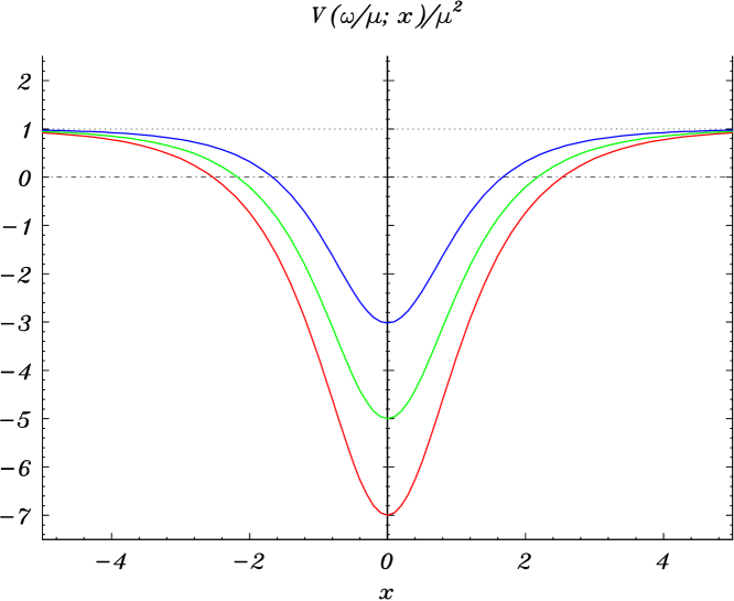
with $\omega=\sqrt{k^{2}+\mu^{2}}$ as before. Note that the potential depends on the momentum of the incoming particle, as shown in Fig. 2.

Figure 2: The normalized potential $V(\omega/\mu;x)/\mu^{2}$ of eq. (4), for $\omega/\mu=$1.01 (upper), 2 (middle) and 3 (lower).

5 Numerical Results

The usual textbook prescription for studying quantum mechanical scattering in one dimension [16] is to start at $t={-}\infty$ with an incoming wave $e^{ikx}$ at $x\sim{-}\infty$. One then analyzes the outgoing waves at $t={+}\infty$, i.e. the transmitted wave $T\,e^{ikx}$ for $x\sim{+}\infty$, and the reflected wave $R\,e^{-ikx}$ for $x\sim{-}\infty$. $T$ is the transition amplitude and $R$ is the reflection amplitude, with

$$|T|^{2}+|R|^{2}=1$$ (59)

ensured by unitarity.

It turns out that for numerical solution of the scattering problem it is more convenient to take the coefficient of the outgoing wave at $x\sim{+}\infty$ to be 1, instead of the $T$ prefactor, and integrate eq. (57) backward, reading off the $T$ and $R$ amplitudes from the solution at $x\sim{-}\infty$.

We thus use

$$v_{j}(x) = e^{ikx},\qquad\qquad\phantom{aaaaaaaaaa}\,\,x\,\to\,{+}\infty$$

(60)

$$v_{j}(x) = {1\over T}\,e^{ikx}+{R\over T}\,e^{-ikx},\qquad\qquad x\,\to\,{-}\infty$$

Since the potential is symmetric, the symmetric and anti-symmetric scattering amplitudes don’t mix, yielding two independent phase shifts $\delta_{S}$ and $\delta_{A}$, respectively. This leads to

$$T = {1\over 2}\left(e^{i\delta_{S}}+e^{i\delta_{A}}\right)$$

(61)

$$R = {1\over 2}\left(e^{i\delta_{S}}-e^{i\delta_{A}}\right)$$

Define

$$\delta_{\pm}={1\over 2}\left(\delta_{S}{\pm}\delta_{A}\right)$$ (62)

Then

$$T = e^{i\delta_{+}}\cos{\delta_{-}}$$

(63)

$$R = ie^{i\delta_{+}}\sin{\delta_{-}}$$

Note that $R/T$ is purely imaginary. The transmission and reflections probabilities are

$$|T|^{2} = \cos^{2}{\delta_{-}}$$

(64)

$$|R|^{2} = \sin^{2}{\delta_{-}}$$

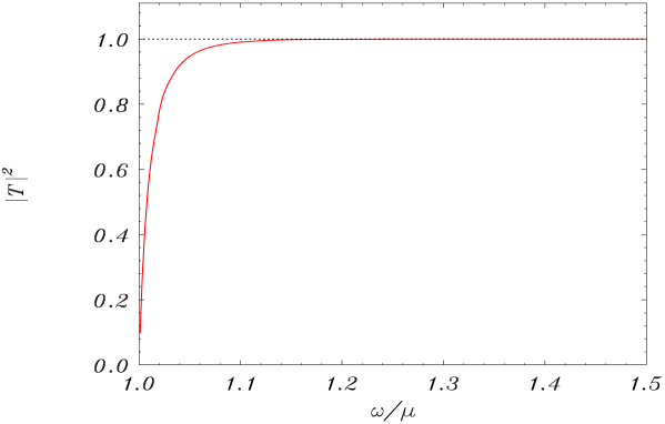
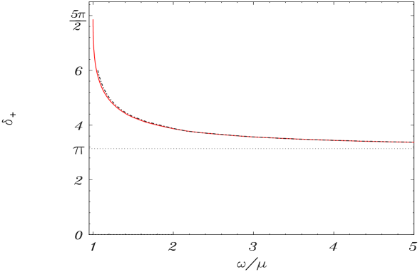
The numerical results for the transmission probability $|T|^{2}$ and for the phase of $T$, $\delta_{+}$ are presented in fig. 3. For comparison and as an extra check we also plot the WKB result for $\delta_{+}$. Note that no resonance appears.

Note that the asymptotic value of the phase shift is $\pi$. This can also be obtained from a WKB calculation, which becomes exact at infinite energies.

Figure 3: Scattering by the potential eq. (4) as function of the normalized energy $\omega/\mu$. Upper plot: transmission probability $|T|^{2}$;  lower plot: phase of $T$, $\delta_{+}$ (continuous line). Also shown is the approximate result for $\delta_{+}$ from WKB (dot-dashed line).

References

• [1] For reviews, see Extended Systems In Field Theory, Proc. Paris meeting, June 16-21, 1975, J.L. Gervais and A. Neveu, Eds., Phys. Rept.  23 (1976) 237.
• [2] R. Rajaraman, Solitons and Instantons: an Introduction to Solitons and Instantons in Quantum Field Theory, North-Holland, 2nd Ed., 1987.
• [3] T. H. Skyrme, Proc. Roy. Soc. Lond. A 260, 127 (1961).
• [4] E. Witten, Nucl. Phys. B 160, 57 (1979).
• [5] For an application of this procedure to the Skyrme model, see G. S. Adkins, C. R. Nappi and E. Witten, Nucl. Phys. B 228, 552 (1983).
• [6] M. P. Mattis and M. Karliner, Phys. Rev. D 31, 2833 (1985);
• [7] M. Karliner and M. P. Mattis, Phys. Rev. Lett.  56, 428 (1986).
• [8] M. Karliner and M. P. Mattis, Phys. Rev. D 34, 1991 (1986).
• [9] H. Walliser and G. Eckart, Nucl. Phys. A 429 (1984) 514.
• [10] G. ’t Hooft, Nucl. Phys. B 75, 461 (1974).
• [11] G. D. Date, Y. Frishman and J. Sonnenschein, Nucl. Phys. B 283, 365 (1987);
• [12] Y. Frishman and J. Sonnenschein, Nucl. Phys. B 294, 801 (1987).
• [13] Y. Frishman and M. Karliner, Nucl. Phys. B 344, 393 (1990).
• [14] J. R. Ellis, Y. Frishman, A. Hanany and M. Karliner, Nucl. Phys. B 382, 189 (1992) [arXiv:hep-ph/9204212].
• [15] Y. Frishman and J. Sonnenschein, Phys. Rept.  223, 309 (1993) [arXiv:hep-th/9207017].
• [16] L.D. Landau and E.M. Lifshitz, Quantum Mechanics: non-relativistic theory, 3rd ed., §23 and §25, Pergamon Press, 1977.
• [17] S.Novikov, S.V.Manakov, L.P.Pitaevskii and V.E.Zakharov, Theory of Solitons: The Inverse Scattering Method, New York: Consultants Bureau, 1984.
• [18] R.L. Jaffe, An Algebraic Approach to Reflectionless Potentials in One Dimension, unpublished notes; available at www-ctp.mit.edu/$\tilde{\phantom{a}}$jaffe/8059_98/Sample_materials/SamplePaper.pdf .
• [19] S. E. Trullinger and R. J. Flesch, J. Math. Phys.  28, 1683 (1987).