Cluster Percolation and Chiral Phase Transition

Abstract

The Meron Cluster algorithm solves the sign problem in a class of interacting fermion lattice models with a chiral phase transition. Within this framework, we study the geometrical features of the clusters built by the algorithm, that suggest the occurrence of a generalized percolating phase transition at the chiral critical temperature in close analogy with Fortuin-Kasteleyn percolation in spin models.

A fundamental difficulty in the Monte Carlo study of fermion lattice models is the sign problem due to the fluctuating sign of the statistical weight of fermion configurations [1]. Recently, the Meron Cluster algorithm (MCA) [2, 3] has been proposed as an effective solution to the sign problem in a class of interacting models. In particular, here, we focus on a $2+1$ dimensional model with a second order phase transition associated to the dynamical breaking of a discrete chiral symmetry [4].

Like all cluster algorithms for lattice models, MCA defines clusters of sites used as effective non-local degrees of freedom to update configurations without critical slowing down. For a given observable, the sign problem is cured by restricting the Monte Carlo sampling to specific topological sectors that give contributions not canceling in pairs due to the fermion sign. The relevant topological charge is the so-called meron number that we shall define later. The rules that assure convergence to the correct Boltzmann equilibrium distribution determine a well defined cluster dynamics. From the study of lattice spin models we know that this artificial dynamics can be surprisingly rich; in fact, experience in that field suggests the existence of a purely geometrical phase transition concerning the algorithm clusters and underlying the physical thermal transition [5, 6, 7].

The simplest example of such a scenario is the 2D Ising model where clusters can be defined in a natural way as sets of nearest neighboring aligned spins and admit a physical interpretation as real ordered domains. At the thermal transition temperature these clusters percolate [8], but since the critical exponents do not coincide with the thermal ones [9], a complete equivalence of the two transitions cannot be claimed. In three dimensions, the comparison is even worse and also the two critical temperatures are slightly different [10]. To find a geometrical transition occurring at the thermal critical point with the same critical exponents, generalized clusters must be defined [11], like the Fortuin-Kasteleyn bond clusters and their extensions [5, 6]. The equivalence between the thermal phase transition and a suitable percolative process can then be extended to models with continuous rotational or gauge invariance [7].

Similar investigations lack for fermionic models with sign problems because cluster algorithms have not been available until MCA. Here, for the first time, we aim to the identification of a geometrical transition in the MCA dynamics and look for critical phenomena defined in terms of cluster shapes. On the other hand, we must keep into account at least the global configuration signs because they are the only memory of the fact that the model is fermionic and allow to tell it from its bosonized counterpart free of sign problems. Besides, apart from the sign problem, the rules to build clusters in MCA are not precisely the same as for Fortuin-Kasteleyn clusters and the existence of a transition is non trivial.

The model we study describes relativistic staggered fermions, hopping on a $2+1$ dimensional lattice with $L^{2}$ spatial sites, described in [4]. The Hamiltonian is

$$H = \sum_{x}\sum_{i=1,2}\left\{\eta_{x,i}(c^{\dagger}_{x}c_{x+\hat{\i}}+h.c.)+\right.$$ (1)

$$+ \left.G\left(n_{x}-\frac{1}{2}\right)\left(n_{x+\hat{\i}}-\frac{1}{2}\right)\right\},$$ (2)

where $n_{x}=c_{x}^{\dagger}c_{x}$ is the occupation number at site $x$, $\eta_{x,i}$ are the Kawamoto-Smit phases $\eta_{x,1}=1$, $\eta_{x,2}=(-1)^{x_{1}}$ and the operators $c$, $c^{\dagger}$ obey standard anti-commutation relations $\{c_{x},c_{y}\}=0$, $\{c_{x},c_{y}^{\dagger}\}=\delta_{x,y}$. In the following we shall consider the case $G=1$ and adopt periodic boundary conditions.

The partition function $\mbox{Tr}\ e^{-\beta H}$ can be computed by Trotter splitting that maps the quantum model to a statistical system on a $2+1$ dimensional lattice with $L^{2}\times T$ sites. The temporal lattice spacing is $\varepsilon=4\beta/T$. The limit $\varepsilon\to 0$ must be taken at fixed $\beta$ with $T\to\infty$. In practice, we shall present results obtained at the fixed value $T=40$ where $\beta$ can cover the transition point with reasonably small $\varepsilon$ [4].

Each configuration is specified by the occupation numbers ${\bf n}=\{n_{x,t}\}$ and carries a sign $\sigma({\bf n})=\pm 1$, source of the sign-problem. To update a configuration, sites are clustered according to definite rules depending on $\beta$ and discussed in details in [3]. Each cluster is then independently flipped: with probability $1/2$ we apply the global transformation $n_{x,t}\to 1-n_{x,t}$ to all of its sites. Clusters whose flip changes $\sigma({\bf n})$ are defined merons.

The chiral phase transition can be analyzed by studying the asymptotic volume dependence of the susceptibility $\chi$. Defining the chiral condensate in the configuration ${\bf n}=\{n_{x,t}\}$ as

$$Z({\bf n})=\frac{\varepsilon}{4}\sum_{x,t}(-1)^{x_{1}+x_{2}}\left(n_{x,t}-\frac{1}{2}\right),$$ (3)

the chiral susceptibility $\chi$ is given by

$$\chi=\frac{1}{\beta L^{2}}\frac{\langle(Z({\bf n})^{2})\ \sigma({\bf n})\rangle}{\langle\sigma({\bf n})\rangle}.$$ (4)

An improved estimator of $\chi$ free of sign problems can be built by writing $Z({\bf n})$ as a sum over clusters $Z({\bf n})=\sum_{C}Z_{C}$ and taking its average over $2^{N_{C}}$ possible flips, where $N_{C}$ is the number of the clusters. Then, $\chi$ gets contributions from sectors with meron number $N=0,2$:

$$\chi=\frac{1}{\beta L^{2}}\frac{\langle\sum_{C}Z_{C}^{2}\ \delta_{N,0}+2|Z_{C_{1}}Z_{C_{2}}|\ \delta_{N,2}\rangle}{\langle\delta_{N,0}\rangle},$$ (5)

where, for $N=2$, $C_{1}$, $C_{2}$ are the two merons.

From numerical simulations, apart from rather small scaling violations, $\chi$ obeys the Finite Size Scaling (FSS) law $\chi=L^{\gamma}f_{\chi}(L(\beta-\beta_{th}))$ with the exponent $\gamma=7/4$, characteristic of the 2D Ising universality class [12]. Numerical simulations locate the chiral $\beta$ at $\beta_{th}=2.43(1)$ [4](the subscript “th” stands for “thermal”).

To detect a possible purely geometrical transition, we study quantities $Q$ that depend only on the cluster shape and not on their internal occupation numbers. Since cluster flips do not change $Q$ and meron flips change the sign of $\sigma({\bf n})$, the improved estimator of $Q$ is

$$\frac{\langle Q({\bf n})\ \sigma({\bf n})\rangle}{\langle\sigma({\bf n})\rangle}=\frac{\langle Q({\bf n})\ \delta_{N,0}\rangle}{\langle\delta_{N,0}\rangle}\equiv\mbox{\bf E}_{0}(Q),$$ (6)

that is the average restricted to the zero meron sector.

The simplest set of geometrical quantities that we can study are the moments $M_{n}=\mbox{\bf E}_{0}\left(\sum_{C}|C|^{n}\right)$ of the normalized cluster size $|C|=\mbox{Vol}(C)/T$ where $\mbox{Vol}(C)$ is the number of sites in $C$.

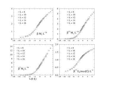
FIG. 1.: FSS analysis of $M_{n}$ and $\mbox{\bf E}_{0}(\max|C|)$.

We perform simulations to compute numerically $\{M_{n}\}_{n=2,3,4}$ and also $\mbox{\bf E}_{0}(\max|C|)$. We work on lattices with $L=8$, $10$, $12$, $14$, $16$ in the range $1.5<\beta<3.0$ and presented about $1.5\cdot 10^{5}$ measures per point. Fig. (1) shows the numerical data supporting as a first result the remarkable validity of the empirical scaling relations:

$$\beta^{n/2}\ M_{n} = L^{n\rho}\ f_{n}(y),\quad n\geq 2,$$ (7)

$$\beta^{1/2}\ \mbox{\bf E}_{0}(\max|C|) = L^{\rho}\ h(y)$$ (8)

in terms of the scaling variable $y=L(\beta-\beta_{c})$. This scaling behavior defines an order parameter of the geometrical phase transition. The results for the exponent $\rho$ and the critical $\beta_{c}$ are $\rho=1.71(5)$ and $\beta_{c}=2.42(5)$. Within errors, $\rho$ is consistent with the exact 2D Ising exact value $\gamma=7/4$. We also find $\beta_{c}\simeq\beta_{th}$ with an accuracy that can be appreciated by looking at Fig. (2).

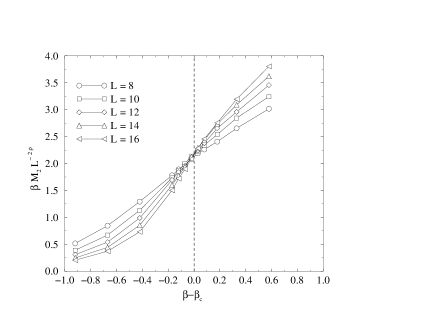
FIG. 2.: Data crossing for $M_{2}$ with different $L$. By virtue of the scaling law Eq. (7), at $\beta=\beta_{c}$ the quantity $\beta M_{2}L^{-2\rho}$ is independent on $L$.

The ratios $R_{n}=M_{2}^{1/2}/M_{n}^{1/n}$ for $n=3,4$ and $R_{\infty}=M_{2}^{1/2}/\mbox{\bf E}_{0}(\max|C|)$ are shown in Fig. (3).

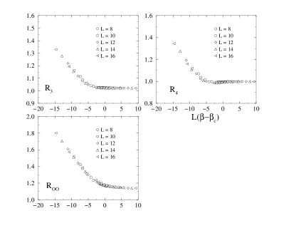
FIG. 3.: Ratios $R_{n}$ and $R_{\infty}$. $M_{n}^{1/n}$ is well approximated by the contribution of the largest cluster beyond the critical point.

The plots strongly indicate that $R_{n}$ are independent on $L$ at fixed $y$ in agreement with Eq. (7).

It can be checked that, at $\beta=\beta_{c}$, $M_{n}$ receives the main contribution from a small set of large clusters growing like $L^{\rho}$, and the fact that the ratios $R_{n}(y)\rightarrow 1$ as $y$ grows, simply means that this contribution is more and more dominant. We briefly summarize this behavior by saying that the clusters are percolating. Following [13], further information on the critical ensemble can be obtained by studying the cluster distribution

$$n_{s}=\mbox{\bf E}_{0}(\#\ \mbox{number of clusters $C$ with $\mbox{Vol}(C)=s$}).$$ (9)

In Fig. (4) we show that the simple law

$$n_{s}=L^{-\rho}f\left(\frac{s}{L^{\rho}}\right),$$ (10)

is well satisfied for $s/L^{\rho}\gg 1$ .

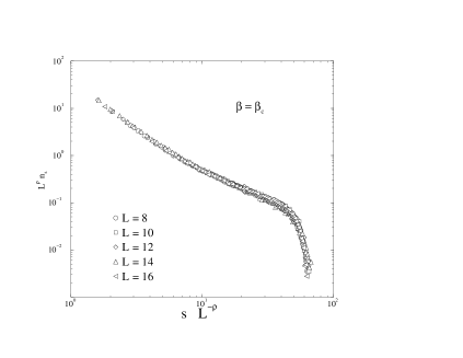
FIG. 4.: FSS plot of $n_{s}$. The curves are obtained after averaging over blocks of 10 subsequent sizes. In the region with $L^{\rho}<s<40\ L^{\rho}$, $n_{s}$ decreases roughly algebraically; beyond the knee at $s\simeq 40\ L^{\rho}$ the distribution falls down quickly. The critical region is dominated by the clusters at the right edge of the plot.

The critical cluster distribution $n_{s}$ decreases not faster than algebraically with $s$ until $s\simeq 40\ L^{\rho}$ where the final large cluster tail is reached and $n_{s}$ falls down quickly.

If one takes into account that the leading contribution to $\{M_{n}\}_{n\geq 2}$ actually comes from the region where $s/L^{\rho}\gg 1$, observing that $M_{n}=\sum_{s}s^{n}n_{s}$ and using Eq. (10) we obtain a $L$-dependence consistent with Eq. (7).

There are many small clusters and one can check that the normalized number of clusters $\beta\ \mbox{\bf E}_{0}(N_{C})/L^{2}$ depends mildly on $L$ for a wide range of $\beta$ and $L$.

It is interesting to analyze what happens to the typical cluster configurations when $\beta$ is gradually increased toward the critical point. At small $\beta$, almost all bonds that build the clusters are set in the temporal direction. In physical terms the fermions hop from the initial positions to neighboring ones with small probability. Sites simply tend to cluster in $L^{2}$ straight vertical lines with $T$ sites. As $\beta\to\beta_{c}$, the vertical clusters start merging and breaking and form complicated structures with large dispersion in the cluster size distribution. This process can be seen in Fig. (5):

FIG. 5.: Two elementary clusters with equal dimension $T$, first merge into a single cluster, then break apart in two clusters with very different dimension.

two vertical clusters with $\mbox{Vol}(C)=T$ undergo a two step process allowed by the cluster rules [2]. In the end, they give rise to a large cluster with $\mbox{Vol}(C)=2T-4$ and a small one with 4 sites. After many processes of this kind we find a few large clusters surrounded by a gas of smaller clusters. In Fig. ( 6)

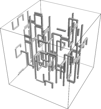
FIG. 6.: A typical largest link configuration for the $8^{2}\times 40$ lattice at $\beta=\beta_{c}$.

we show a typical largest cluster obtained at $\beta=2.5$ on the $8^{2}\times 40$ lattice.

Geometrical quantities that can measure this dispersion effect are the cumulants $\{G_{n}\}_{n\geq 1}$ of the cluster size distribution defined as

$$\sum_{n\geq 1}\frac{\lambda^{n}}{n!}G_{n}=\mbox{\bf E}_{0}\left\{\log\left(\sum_{n\geq 0}\frac{\lambda^{n}}{n!}\frac{1}{N_{C}}\sum_{C}|C|^{n}\right)\right\}.$$ (11)

In our study we do not consider the cumulant $G_{1}$, whose behavior is determined by the the contributions from small clusters, with $s\ll L^{\rho}$.

The next cumulant is the variance

$$G_{2}=\mbox{\bf E}_{0}\left(\frac{1}{N_{C}}\sum_{C}|C|^{2}-\frac{1}{N_{C}^{2}}(\sum_{C}|C|)^{2}\right).$$ (12)

Our data support a FSS law of the form

$$\beta G_{2}=L^{\rho^{\prime}}g_{2}(y),$$ (13)

with $\rho^{\prime}=1.51(4)$, which is compatible with $2\gamma-2$. This exponent can be explained taking account that, analogously to the moment $M_{2}$, the contributions from small clusters are negligible and that, within errors, $\sum_{C}|C|^{2}\sim L^{2\gamma}$ and $N_{C}\sim L^{2}$ .

As we remarked above, when $\beta\rightarrow 0$, the clusters are simple vertical lines and $G_{2}\rightarrow 0$ like $\chi$ does. This fact suggests that it could be interesting to study a possible relationship between these quantities at different $\beta$ values. We remark that, in principle, $G_{2}$ and $\chi$ have different topological origins: $\chi$ is calculated on zero and two merons sector, while $G_{2}$ only on zero-meron sector. Nevertheless, we find that the following empirical relation

$$\chi\simeq 0.15(1)\cdot(\beta\ G_{2})^{\frac{1}{2}\frac{\gamma}{\gamma-1}},$$ (14)

holds for a wide range of parameters $(L,\beta)$ as shown in Fig. (7).

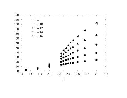
FIG. 7.: Comparison between $\chi$ (empty symbols) and $0.15\cdot(\beta G_{2})^{7/6}$ (full symbols).

In practice, in the region that we have explored, the ratio $\chi/(\beta G_{2})^{7/6}$ is consistent, within errors, with a constant. This result signals an unexpected correlation between different topological sectors. In particular, Eq. (14) could be relevant in the construction of a purely geometrical definition of $\chi$. A FSS study of the higher cumulants $G_{3}$ and $G_{4}$ shows similar scaling laws, but with exponents that are not in simple relation with $\gamma$ and should in principle be matched to the anomalous dimensions of higher operators in the 2D Ising universality class.

To conclude, we have examined the critical behavior of the clusters that arise in the application of the Meron algorithm to a fermion model in $2+1$ dimensions. We have found simple FSS laws that we have explained in terms of a percolative process occurring at the chiral critical temperature. Our data support the results $\rho\simeq\gamma$, $\rho^{\prime}\simeq 2\gamma-2$, as well as the empirical relation Eq. (14) that shows a close correlation between physical and geometrical quantities.

We acknowledge S. Chandrasekharan, K. Holland and U.J. Wiese for useful discussions about the Meron-Cluster Algorithm and its applications. Financial support from INFN, IS-RM42 is also acknowledged.

REFERENCES

- [1] W. von der Linden, Phys. Rep. 220, 53 (1992).
- [2] S. Chandrasekharan and J. Osborn, Springer Proc. Phys. 86, 28 (2000); S. Chandrasekharan and J. C. Osborn, Phys. Lett. B 496, 122 (2000); S. Chandrasekharan, Chin. J. Phys. 38, 696 (2000); S. Chandrasekharan, Nucl. Phys. Proc. Suppl. 83, 774 (2000); S. Chandrasekharan and U. J. Wiese, Phys. Rev. Lett. 83, 3116 (1999); S. Chandrasekharan, Nucl. Phys. Proc. Suppl. 106, 1025 (2002);
- [3] S. Chandrasekharan, J. Cox, K. Holland and U. J. Wiese, Nucl. Phys. B 576, 481 (2000);
- [4] J. Cox and K. Holland, Nucl. Phys. B 583, 331 (2000).
- [5] P. W. Kasteleyn, C. M. Fortuin, Jour. Phys. Soc. of Japan 26 (Suppl.), 11 (1969); C. M. Fortuin, P. W. Kasteleyn, Physica 57, 536 (1972); C. M. Fortuin, Physica 58, 393 (1972); C. M. Fortuin, Physica 59, 545 (1972).
- [6] R. G. Edwards, A. D. Sokal, Phys. Rev. D 38, 2009 (1988).
- [7] S. Fortunato, H. Satz, Nucl. Phys. Proc. Suppl. 106, 890 (2002); S. Fortunato, F. Karsch, P. Petreczky and H. Satz, Nucl. Phys. Proc. Suppl. 94, 398 (2001); S. Fortunato and H. Satz, Nucl. Phys. B 598, 601 (2001). P. Blanchard et al., J. Phys. A 33, 8603 (2000);
- [8] A. Coniglio, C. R. Nappi, F. Peruggi and L. Russo, Commun. Math. Phys. 51, 315 (1976).
- [9] M. F. Sykes, D. S. Gaunt, Jour. of Phys. A 9, 2131 (1976).
- [10] H. Müller-Krumbhaar, Phys. Lett. A 48, 459 (1974).
- [11] A. Coniglio, W. Klein, Jour. of Phys. A 13, 2775 (1980).
- [12] The first numerical evidence of this result is J. B. Kogut, M. A. Stephanov, C.G. Strouthos, Phys. Rev. D 58, 096001 (1998);
- [13] D. Stauffer, Phys. Rept. 54, 1 (1979).