LU TP 02-21

hep-ph/0205341

revised October 2002

$K\to 3\pi$ Decays in Chiral Perturbation Theory
Johan Bijnens, Pierre Dhonte and Fredrik Persson
Department of Theoretical Physics, Lund University

Sölvegatan 14A, S 22362 Lund, Sweden

The CP conserving amplitudes for the decays $K\to 3\pi$ are calculated in Chiral Perturbation Theory at the next-to-leading order. We present the expressions in a compact form with single parameter functions only. These expressions are then fitted to all available $K\to 2\pi$ and $K\to 3\pi$ data to obtain a fit of the parameters that occur. We compare with the work of Kambor, Missimer and Wyler.

PACS numbers: 13.20.Eb, 12.39.Fe, 14.40.Aq, 11.30.Rd

1 Introduction

Chiral Perturbation Theory (ChPT) is the low-energy effective field theory of the strong interactions. It was introduced in its modern form by Weinberg, Gasser and Leutwyler [1, 2, 3]. It has had many successes and applications. A pedagogical introduction can be found in [4]. The method has been used as well for nonleptonic weak decays. The main work of extending ChPT to the nonleptonic weak interaction was done long ago by Kambor, Missimer and Wyler who worked out the general formalism [5] and applied it to $K\to 2\pi,3\pi$ decays [6]. These results were then used to obtain directly relations between physical observables in [7]. Reviews of applications of ChPT to nonleptonic weak interactions are [8].

Earlier work using current algebra methods or tree level Lagrangians relevant for $K\to 3\pi$ are [9, 10] and references therein. Many new measurements in $K\to 3\pi$ have become available since the work of [6] so an update of the fits of the parameters done there became necessary. The analytical expressions of [6] were never published and have since been lost. This forced us to reevaluate these decays and we present the analytical results here using a simplified form derived using the arguments first used for $\pi\pi$-scattering by Knecht et al. [11]. We then perform a detailed comparison of the expressions with the data and find a reasonable agreement. We point out some directions for future work.

The next section defines our notation and gives a unique list of possible terms at next-to-leading order in ChPT. Section 3 gives the list of decays and the isospin constraints as well as the simplified analytical form valid up till order $p^{6}$ in ChPT. The ambiguities in this simplified form are discussed in detail in App. A. This section also discusses the isospin constraints on the various amplitudes. Our main result, the recalculation of the $K\to 3\pi$ amplitudes is discussed in Sect. 4 where we present the tree level result and work out the independent combinations of the weak $p^{4}$ parameters that occur. The expressions at order $p^{4}$ are still rather cumbersome and are listed in App. B. Section 5 contains a short review of the available data and presents in detail the various fits we have performed to the data. Our conclusions are summarized in the final section.

2 The ChPT Lagrangian

The Lagrangian of ChPT in the strong sector was worked out at next-to-leading order (NLO) in [2] and is given by

$${\cal L}_{S}={\cal L}_{S2}+{\cal L}_{S4}\,,$$ (1)

with

$${\cal L}_{S2} = \frac{F_{0}^{2}}{4}\{\langle D_{\mu}U^{\dagger}D^{\mu}U\rangle+\langle\chi^{\dagger}U+\chi U^{\dagger}\rangle\}\,,$$ (2)

$${\cal L}_{S4} = L_{1}\langle D_{\mu}U^{\dagger}D^{\mu}U\rangle^{2}+L_{2}\langle D_{\mu}U^{\dagger}D_{\nu}U\rangle\langle D^{\mu}U^{\dagger}D^{\nu}U\rangle$$ (3)

$$+L_{3}\langle D^{\mu}U^{\dagger}D_{\mu}UD^{\nu}U^{\dagger}D_{\nu}U\rangle+L_{4}\langle D^{\mu}U^{\dagger}D_{\mu}U\rangle\langle\chi^{\dagger}U+\chi U^{\dagger}\rangle$$

$$+L_{5}\langle D^{\mu}U^{\dagger}D_{\mu}U(\chi^{\dagger}U+U^{\dagger}\chi)\rangle+L_{6}\langle\chi^{\dagger}U+\chi U^{\dagger}\rangle^{2}$$

$$+L_{7}\langle\chi^{\dagger}U-\chi U^{\dagger}\rangle^{2}+L_{8}\langle\chi^{\dagger}U\chi^{\dagger}U+\chi U^{\dagger}\chi U^{\dagger}\rangle$$

$$-iL_{9}\langle F^{R}_{\mu\nu}D^{\mu}UD^{\nu}U^{\dagger}+F^{L}_{\mu\nu}D^{\mu}U^{\dagger}D^{\nu}U\rangle$$

$$+L_{10}\langle U^{\dagger}F^{R}_{\mu\nu}UF^{L\mu\nu}\rangle\,.$$

$\langle A\rangle$ stands for the flavour trace of the matrix $A$, and $F_{0}$ is the pion decay constant in the chiral limit. The special unitary matrix $U$ contains the Goldstone boson fields

$$U=\exp\left(\frac{i\sqrt{2}}{F_{0}}M\right)\,,\quad M=\left(\begin{array}[]{ccc}\frac{1}{\sqrt{2}}\pi^{0}+\frac{1}{\sqrt{6}}\eta&\pi^{+}&K^{+}\\ \pi^{-}&\frac{-1}{\sqrt{2}}\pi^{0}+\frac{1}{\sqrt{6}}\eta&K^{0}\\ K^{-}&\overline{K^{0}}&\frac{-2}{\sqrt{6}}\eta\end{array}\right)\,.$$ (4)

The formalism we use is the external field method of [2] with $s$, $p$, $l_{\mu}$ and $r_{\mu}$ matrix valued scalar, pseudo-scalar, left-handed and right handed vector external fields respectively. These show up in

$$\chi=2B_{0}\left(s+ip\right)\,,$$ (5)

in the covariant derivative

$$D_{\mu}U=\partial_{\mu}U-ir_{\mu}U+iUl_{\mu}\,,$$ (6)

and in the field strength tensor

$$F_{\mu\nu}^{L(R)}=\partial_{\mu}l(r)_{\nu}-\partial_{\nu}l(r)_{\mu}-i\left[l(r)_{\mu},l(r)_{\nu}\right]\,.$$ (7)

For our purpose it suffices to set

$$s=\left(\begin{array}[]{ccc}m_{u}&&\\ &m_{d}&\\ &&m_{s}\end{array}\right)\,,\quad p=0\,,\quad l_{\mu}=r_{\mu}=0\,.$$ (8)

We also define the matrices $u$, $u_{\mu}$ and $\chi_{\pm}$,

$$u_{\mu}=iu^{\dagger}D_{\mu}Uu^{\dagger}=u_{\mu}^{\dagger}\,,\quad u^{2}=U,\quad\chi_{\pm}=u^{\dagger}\chi u^{\dagger}\pm u\chi^{\dagger}u\,.$$ (9)

The ChPT Lagrangian for the weak nonleptonic interactions at lowest order dates back to current algebra days [9] and is

$${\cal L}_{W2}=C\,F_{0}^{4}\,\Bigg{[}G_{8}\langle\Delta_{32}u_{\mu}u^{\mu}\rangle+G_{8}^{\prime}\langle\Delta_{32}\chi_{+}\rangle+G_{27}t^{ij,kl}\,\langle\Delta_{ij}u_{\mu}\rangle\langle\Delta_{kl}u^{\mu}\rangle\Bigg{]}+\mbox{ h.c.}$$

The tensor $t^{ij,kl}$ has as nonzero components

$$t^{21,13}=t^{13,21}=\frac{1}{3}\, \,t^{22,23}=t^{23,22}=-\frac{1}{6}\,;$$ ;

$$t^{23,33}=t^{33,23}=-\frac{1}{6}\, \,t^{23,11}=t^{11,23}=\frac{1}{3}\,.$$ ; (10)

The matrix $\Delta_{ij}$ is defined as

$$\Delta_{ij}\equiv u\lambda_{ij}u^{\dagger}\,,\quad\left(\lambda_{ij}\right)_{ab}\equiv\delta_{ia}\,\delta_{jb}\,.$$ (11)

We only quote the $|\Delta S|=1$ part here but the others can be obtained by changing the indices in $\Delta_{32}$ and $t^{ij,kl}$ appropriately. The parts with $G_{8}$ and $G_{8}^{\prime}$ transforms as an octet under $SU(3)_{L}$ while the $G_{27}$ part transforms as a 27 under the same group. The term with $G_{8}^{\prime}$ is often referred to as the weak mass term.

The coefficient $C$ is defined such that in the chiral and large $N_{c}$ limits $G_{8}=G_{27}=1$,

$$C=-\frac{3}{5}\,\frac{G_{F}}{\sqrt{2}}V_{ud}\,V_{us}^{*}\,.$$ (12)

The correspondence with the parameters $c_{2}$ and $c_{3}$ of [5, 6] is

$$c_{2}=CF_{0}^{4}G_{8}\,\quad c_{3}=-\frac{1}{6}CF_{0}^{4}G_{27}\,.$$ (13)

The NLO nonleptonic weak Lagrangian was first worked out in [5] but the basis given there was redundant. Subsequent work on a less redundant basis was [12]. A fully nonredundant basis for the octet part was presented in [13]. We will use the basis of [13] for the octet part and use the notation of [5] for the 27 part, but keep only the nonredundant terms as derived in [12]. The NLO weak ChPT Lagrangian, quoting only the terms relevant for $K\to 2\pi$ and $K\to 3\pi$ decays, is

$${\cal L}^{(4)}_{\Delta S=1} = C\,F_{0}^{2}\,\Bigg{\{}G_{8}\Big{[}N_{1}{\cal O}^{8}_{1}+N_{2}{\cal O}^{8}_{2}+N_{3}{\cal O}^{8}_{3}+N_{4}{\cal O}^{8}_{4}N_{5}{\cal O}^{8}_{5}+N_{6}{\cal O}^{8}_{6}+N_{7}{\cal O}^{8}_{7}$$ (14)

$$+N_{8}{\cal O}^{8}_{8}+N_{9}{\cal O}^{8}_{9}+N_{10}{\cal O}^{8}_{10}+N_{11}{\cal O}^{8}_{11}+N_{12}{\cal O}^{8}_{12}+N_{13}{\cal O}^{8}_{13}\Big{]}$$

$$+G_{27}\,\Big{[}D_{1}{\cal O}^{27}_{1}+D_{2}{\cal O}^{27}_{2}+D_{4}{\cal O}^{27}_{4}+D_{5}{\cal O}^{27}_{5}+D_{6}{\cal O}^{27}_{6}+D_{7}{\cal O}^{27}_{7}+D_{26}{\cal O}^{27}_{26}$$

$$+D_{27}{\cal O}^{27}_{27}+D_{28}{\cal O}^{27}_{28}+D_{29}{\cal O}^{27}_{29}+D_{30}{\cal O}^{27}_{30}+D_{31}{\cal O}^{27}_{31}\Big{]}\Bigg{\}}+\mbox{h.c.}\,.$$

The octet operators are

$${\cal O}^{8}_{1} = \langle\Delta_{32}u_{\mu}u^{\mu}u_{\nu}u^{\nu}\rangle\,,$$

$${\cal O}^{8}_{2} = \langle\Delta_{32}u_{\mu}u_{\nu}u^{\nu}u^{\mu}\rangle\,,$$

$${\cal O}^{8}_{3} = \langle\Delta_{32}u_{\mu}u_{\nu}\rangle\langle u^{\mu}u^{\nu}\rangle\,,$$

$${\cal O}^{8}_{4} = \langle\Delta_{32}u_{\mu}\rangle\langle u_{\nu}u^{\mu}u^{\nu}\rangle\,,$$

$${\cal O}^{8}_{5} = \langle\Delta_{32}(\chi_{+}u_{\mu}u^{\mu}+u_{\mu}u^{\mu}\chi_{+})\rangle\,,$$

$${\cal O}^{8}_{6} = \langle\Delta_{32}u_{\mu}\rangle\langle u^{\mu}\chi_{+}\rangle\,,$$

$${\cal O}^{8}_{7} = \langle\Delta_{32}\chi_{+}\rangle\langle u_{\mu}u^{\mu}\rangle\,,$$

$${\cal O}^{8}_{8} = \langle\Delta_{32}u_{\mu}u^{\mu}\rangle\langle\chi_{+}\rangle\,,$$

$${\cal O}^{8}_{9} = \langle\Delta_{32}(\chi_{-}u_{\mu}u^{\mu}-u_{\mu}u^{\mu}\chi_{-})\rangle\,,$$

$${\cal O}^{8}_{10} = \langle\Delta_{32}\chi_{+}\chi_{+}\rangle\,,$$

$${\cal O}^{8}_{11} = \langle\Delta_{32}\chi_{+}\rangle\langle\chi_{+}\rangle\,,$$

$${\cal O}^{8}_{12} = \langle\Delta_{32}\chi_{-}\chi_{-}\rangle\,,$$

$${\cal O}^{8}_{13} = \langle\Delta_{32}\chi_{-}\rangle\langle\chi_{-}\rangle\,.$$ (15)

The 27 operators are

$${\cal O}^{27}_{1} = t^{ij,kl}\langle\Delta_{ij}\chi_{+}\rangle\langle\Delta_{kl}\chi_{+}\rangle\,,$$

$${\cal O}^{27}_{2} = t^{ij,kl}\langle\Delta_{ij}\chi_{-}\rangle\langle\Delta_{kl}\chi_{-}\rangle\,,$$

$${\cal O}^{27}_{4} = t^{ij,kl}\langle\Delta_{ij}u_{\mu}\rangle\langle\Delta_{kl}(u^{\mu}\chi_{+}+\chi_{+}u^{\mu})\rangle\,,$$

$${\cal O}^{27}_{5} = t^{ij,kl}\langle\Delta_{ij}u_{\mu}\rangle\langle\Delta_{kl}(u^{\mu}\chi_{-}-\chi_{-}u^{\mu})\rangle\,,$$

$${\cal O}^{27}_{6} = t^{ij,kl}\langle\Delta_{ij}\chi_{+}\rangle\langle\Delta_{kl}u_{\mu}u^{\mu}\rangle\,,$$

$${\cal O}^{27}_{7} = t^{ij,kl}\langle\Delta_{ij}u_{\mu}\rangle\langle\Delta_{kl}u^{\mu}\rangle\langle\chi_{+}\rangle\,,$$

$${\cal O}^{27}_{26} = t^{ij,kl}\langle\Delta_{ij}u_{\mu}u^{\mu}\rangle\langle\Delta_{kl}u_{\nu}u^{\nu}\rangle\,,$$

$${\cal O}^{27}_{27} = t^{ij,kl}\langle\Delta_{ij}(u_{\mu}u_{\nu}+u_{\nu}u_{\mu})\rangle\langle\Delta_{kl}(u^{\mu}u^{\nu}+u^{\nu}u^{\mu})\rangle\,,$$

$${\cal O}^{27}_{28} = t^{ij,kl}\langle\Delta_{ij}(u_{\mu}u_{\nu}-u_{\nu}u_{\mu})\rangle\langle\Delta_{kl}(u^{\mu}u^{\nu}-u^{\nu}u^{\mu})\rangle\,,$$

$${\cal O}^{27}_{29} = t^{ij,kl}\langle\Delta_{ij}u_{\mu}\rangle\langle\Delta_{kl}u_{\nu}u^{\mu}u^{\nu}\rangle\,,$$

$${\cal O}^{27}_{30} = t^{ij,kl}\langle\Delta_{ij}u_{\mu}\rangle\langle\Delta_{kl}(u^{\mu}u_{\nu}u^{\nu}+u_{\nu}u^{\nu}u^{\mu})\rangle\,,$$

$${\cal O}^{27}_{31} = t^{ij,kl}\langle\Delta_{ij}u_{\mu}\rangle\langle\Delta_{kl}u^{\mu}\rangle\langle u_{\nu}u^{\nu}\rangle\,.$$ (16)

Notice that some have the opposite sign compared to [5], because of the difference in the definition of $\chi_{i}$ and $P$ of that reference. The basis used in [14] for the octet case is slightly different but related to the one here by

$$\begin{array}[b]{lll}N_{5}=E_{10}-E_{11}\,;&N_{6}=E_{11}+2E_{12}\,;&N_{7}=\frac{1}{2}E_{11}+E_{13}\,;\\ N_{8}=E_{11}\,;&N_{9}=E_{15}\,;&N_{10}=E_{1}-E_{5}\,;\\ N_{11}=E_{2}\,;&N_{12}=-E_{3}+E_{5}\,;&N_{13}=E_{4}\,;\\ N_{36}=E_{5}\,.\end{array}$$ (17)

Notice that there is a small misprint in the relation between the $E_{i}$ and $N_{i}$ in (2.19) of [14] in the relation between $N_{13}$ and $E_{4}$.

The infinities appearing in the loop diagrams are canceled by replacing the coefficients in (3) and (14) by the renormalized coefficients and a subtraction part. The infinities needed in the strong sector were calculated first in [3] and those for the weak sector in [5] and confirmed in [12]. For the terms in Eqs. (3) and (14) they are all of the type

$$X_{i}=(e^{c}\mu)^{-2\epsilon}\left(X_{i}^{r}+x_{i}\frac{1}{16\pi^{2}\epsilon}\right)\,,$$ (18)

with the dimension of space-time $d=4-2\epsilon$ and

$$c=-\frac{1}{2}\left(\ln(4\pi)+\Gamma^{\prime}(1)+1\right)\,,$$ (19)

for $X=L,N,D$. The coefficients are listed in Table 1 [3, 5, 12].

$L_{i}$	$\ell_{i}$	$N_{i}$	$n_{i}$	$D_{i}$	$d_{i}$
1	$-3/64$	1	$-1$	1	$1/12$
2	$-3/32$	2	$1/4$	2	$0$
3	$0$	3	$0$	4	$-3/2$
4	$-1/16$	4	$-1/2$	5	$-1/2$
5	$-3/16$	5	$-3/4-3/8\,(G_{8}^{\prime}/G_{8})$	6	$3/4$
6	$-11/288$	6	$1/8$	7	$-1/2$
7	$0$	7	$9/16-1/4\,(G_{8}^{\prime}/G_{8})$	26	$1/2$
8	$-5/96$	8	$1/4$	27	$1/4$
9	$-1/8$	9	$-3/8+3/8\,(G_{8}^{\prime}/G_{8})$	28	$5/6$
10	$1/8$	10	$-1/3-5/24\,(G_{8}^{\prime}/G_{8})$	29	$-19/$
		11	$13/36-11/36\,(G_{8}^{\prime}/G_{8})$	30	$-5/3$
		12	$5/24-5/24\,(G_{8}^{\prime}/G_{8})$	31	$0$
		13	$0$

Table 1: The coefficients of the subtraction of the infinite parts defined in Eq. (18).

3 Kinematics and Isospin

There are five CP-conserving decays of the type $K\to 3\pi$:

$$K_{L}(k) \to \pi^{0}(p_{1})\pi^{0}(p_{2})\pi^{0}(p_{3})\,,\quad[A^{L}_{000}]\,,$$

$$K_{L}(k) \to \pi^{+}(p_{1})\pi^{-}(p_{2})\pi^{0}(p_{3})\,,\quad[A^{L}_{+-0}]\,,$$

$$K_{S}(k) \to \pi^{+}(p_{1})\pi^{-}(p_{2})\pi^{0}(p_{3})\,,\quad[A^{S}_{+-0}]\,,$$

$$K^{+}(k) \to \pi^{0}(p_{1})\pi^{0}(p_{2})\pi^{+}(p_{3})\,,\quad[A_{00+}]\,,$$

$$K^{+}(k) \to \pi^{+}(p_{1})\pi^{+}(p_{2})\pi^{-}(p_{3})\,,\quad[A_{++-}]\,,$$ (20)

where we have indicated the four momentum defined for each particle and the symbol we will use for the amplitude. The $K^{+}$ decays have an obvious counterpart in $K^{-}$ decays.

The kinematics is normally treated using

$$s_{1}=\left(k-p_{1}\right)^{2}\,,\quad s_{2}=\left(k-p_{2}\right)^{2}\,,\quad s_{3}=\left(k-p_{3}\right)^{2}\,.$$ (21)

The amplitudes are often expanded in terms of the Dalitz plot variables $x$ and $y$ defined via

$$x=\frac{s_{2}-s_{1}}{m_{\pi^{+}}^{2}}\,,\quad y=\frac{s_{3}-s_{0}}{m_{\pi^{+}}^{2}}\,,\quad s_{0}=\frac{1}{3}\left(m_{K}^{2}+m_{\pi^{1}}^{2}+m_{\pi^{2}}^{2}+m_{\pi^{3}}^{2}\right)\,,$$ (22)

where the kaon mass and the pion masses in $s_{0}$ are those from the particles appearing in the decay under consideration.

The amplitudes for $K_{L}\to\pi^{+}\pi^{-}\pi^{0},K^{+}\to\pi^{+}\pi^{+}\pi^{-}$ and $K^{+}\to\pi^{0}\pi^{0}\pi^{+}$ are symmetric under the interchange of the first two pions because of CP or Bose-symmetry. The amplitude for $K_{L}\to\pi^{0}\pi^{0}\pi^{0}$ is obviously symmetric under the interchange of all three final state particles and the one for $K_{S}\to\pi^{+}\pi^{-}\pi^{0}$ is antisymmetric under the interchange of $\pi^{+}$ and $\pi^{-}$ because of CP.

Isospin invariance does give some constraints on the amplitudes [15, 16, 17]. These can be written as

$$A^{L}_{000}(s_{1},s_{2},s_{3}) = 3A_{n}(s_{1},s_{2},s_{3})\,,$$

$$A^{L}_{+-0}(s_{1},s_{2},s_{3}) = A_{n}(s_{1},s_{2},s_{3})-B_{n}(s_{1},s_{2},s_{3})\,,$$

$$A^{S}_{+-0}(s_{1},s_{2},s_{3}) = C_{0}(s_{1},s_{2},s_{3})+\frac{2}{3}\left[B_{t}(s_{3},s_{2},s_{1})-B_{t}(s_{3},s_{1},s_{2})\right]\,,$$

$$A_{00+}(s_{1},s_{2},s_{3}) = A_{c}(s_{1},s_{2},s_{3})-B_{c}(s_{1},s_{2},s_{3})+B_{t}(s_{1},s_{2},s_{3})\,,$$

$$A_{++-}(s_{1},s_{2},s_{3}) = 2A_{c}(s_{1},s_{2},s_{3})+B_{c}(s_{1},s_{2},s_{3})+B_{t}(s_{1},s_{2},s_{3})\,.$$ (23)

The functions $A_{c,n}$ are fully symmetric in $s_{1},s_{2},s_{3}$. $C_{0}$ is fully antisymmetric and $B_{c,n,t}(s_{1},s_{2},s_{3})$ is symmetric under the interchange $s_{1}\leftrightarrow s_{2}$ and satisfies the relation

$$B_{i}(s_{1},s_{2},s_{3})+B_{i}(s_{2},s_{3},s_{1})+B_{i}(s_{3},s_{1},s_{2})=0\,.$$ (24)

$A_{c,n}$ and $B_{c,n}$ belong to the $I=1$ final state, $B_{t}$ to the $I=2$ final state and $C_{0}$ to the $I=0$ final state.

A further simplification can be obtained by observing that the imaginary parts of loop diagrams in ChPT do not contain $\ell\geq 2$ until at least ${\cal O}(p^{8})$. This allows to rewrite the amplitudes in a way that only contains functions of single variables and is fully correct up to ${\cal O}(p^{6})$. The underlying arguments are the same as the ones used for a similar decomposition for $\pi\pi$ scattering by [11].

$$A^{L}_{000}(s_{1},s_{2},s_{3}) = M_{0}(s_{1})+M_{0}(s_{2})+M_{0}(s_{3})\,,$$

$$A^{L}_{+-0}(s_{1},s_{2},s_{3}) = M_{1}(s_{3})+M_{2}(s_{1})+M_{2}(s_{2})+M_{3}(s_{1})(s_{2}-s_{3})+M_{3}(s_{2})(s_{1}-s_{3})\,,$$

$$A^{S}_{+-0}(s_{1},s_{2},s_{3}) = M_{4}(s_{1})-M_{4}(s_{2})+M_{5}(s_{1})(s_{2}-s_{3})-M_{5}(s_{2})(s_{1}-s_{3})$$

$$+M_{6}(s_{3})(s_{1}-s_{2})\,,$$

$$A_{00+}(s_{1},s_{2},s_{3}) = M_{7}(s_{3})+M_{8}(s_{1})+M_{8}(s_{2})+M_{9}(s_{1})(s_{2}-s_{3})+M_{9}(s_{2})(s_{1}-s_{3})\,,$$

$$A_{++-}(s_{1},s_{2},s_{3}) = M_{10}(s_{3})+M_{11}(s_{1})+M_{11}(s_{2})+M_{12}(s_{1})(s_{2}-s_{3})+M_{12}(s_{2})(s_{1}-s_{3})\,.$$

The expressions for the various amplitudes become significantly shorter when written explicitly in this form. Comparing (3) and (3) gives

$$A_{n}(s_{1},s_{2},s_{3}) = \sum_{i=1,3}\frac{1}{3}M_{0}(s_{i})\,,$$

$$A_{c}(s_{1},s_{2},s_{3}) = \sum_{i=1,3}\frac{1}{3}\left(M_{7}(s_{i})+2M_{8}(s_{i})\right)\,,$$

$$B_{n}(s_{1},s_{2},s_{3}) = B_{n1}(s_{1})+B_{n1}(s_{2})-2B_{n1}(s_{3})+B_{n2}(s_{1})(s_{2}-s_{3})+B_{n2}(s_{2})(s_{1}-s_{3})\,,$$

$$B_{n1}(s) = \frac{1}{3}\left(M_{1}(s)-M_{2}(s)\right)\,,$$

$$B_{n2}(s) = -M_{3}(s)\,,$$

$$B_{c}(s_{1},s_{2},s_{3}) = B_{c1}(s_{1})+B_{c1}(s_{2})-2B_{c1}(s_{3})+B_{c2}(s_{1})(s_{2}-s_{3})+B_{c2}(s_{2})(s_{1}-s_{3})\,,$$

$$B_{c1}(s) = \frac{1}{6}\left(M_{7}(s)-M_{8}(s)-M_{10}(s)+M_{11}(s)\right)\,$$

$$B_{c2}(s) = \frac{1}{2}\left(-M_{9}(s)+M_{12}(s)\right)\,,$$

$$B_{t}(s_{1},s_{2},s_{3}) = B_{t1}(s_{1})+B_{t1}(s_{2})-2B_{t1}(s_{3})+B_{t2}(s_{1})(s_{2}-s_{3})+B_{t2}(s_{2})(s_{1}-s_{3})\,,$$

$$B_{t1}(s) = \frac{1}{6}\left(-M_{7}(s)+M_{8}(s)-M_{10}(s)+M_{11}(s)\right)\,$$

$$B_{t2}(s) = \frac{1}{2}\left(M_{9}(s)+M_{12}(s)\right)\,,$$

$$C_{0}(s_{1},s_{2},s_{3}) = C_{01}(s_{3})(s_{1}-s_{2})+C_{01}(s_{1})(s_{2}-s_{3})+C_{01}(s_{2})(s_{3}-s_{1})\,,$$

$$C_{01}(s) = \frac{1}{3}\left(2M_{5}(s)+M_{6}(s)\right)$$ (26)

and the relations

$$M_{0}(s) = M_{1}(s)+2M_{2}(s)\,,$$

$$2M_{7}(s)+4M_{8}(s) = M_{10}(s)+2M_{11}(s)\,,$$

$$M_{4}(s) = \frac{1}{3}\left(M_{7}(s)-M_{8}(s)+M_{10}(s)-M_{11}(s)\right)\,$$

$$M_{5}(s)-M_{6}(s) = M_{9}(s)+M_{12}(s)\,.$$ (27)

The split-up between the polynomial parts in (3) has some ambiguity as discussed in App. A. The same ambiguity appears in the rewriting of the $B_{cnt}$ functions in single variable parts and can affect the last two relations in (3). The results given explicitly in App. B are brought in a form satisfying the relations (3) using this freedom.

4 Analytical Results

The lowest order result is well known and follows from the diagrams in Fig.1.

Figure 1: The tree level diagrams for $K\to 3\pi$. A filled square is a vertex from ${\cal L}_{W2}$ and a filled circle from ${\cal L}_{S2}$.

The Feynman amplitude at tree level for $A^{L}_{000}$ is

$$\left.M_{0}(s)\right|_{p^{2}}=i\frac{CF_{0}^{4}}{F_{\pi}^{3}F_{K}}\,\frac{1}{3}\left(G_{8}-G_{27}\right)m_{K}^{2}\,.$$ (28)

A choice for $A^{L}_{+-0}$ compatible with the relations (3) and (28) is

$$\left.M_{1}(s)\right|_{p^{2}} = i\frac{CF_{0}^{4}}{F_{\pi}^{3}F_{K}}\,\frac{1}{3}\left(G_{8}-G_{27}\right)m_{K}^{2}\,,$$

$$\left.M_{2}(s)\right|_{p^{2}} = 0\,,$$

$$\left.M_{3}(s)\right|_{p^{2}} = i\frac{CF_{0}^{4}}{F_{\pi}^{3}F_{K}}\,\left\{-\frac{G_{8}}{3}+\frac{G_{27}}{6}\,\frac{-3m_{K}^{2}+8m_{\pi}^{2}}{m_{K}^{2}-m_{\pi}^{2}}\right\}$$ (29)

The tree level result for $A^{S}_{+-0}$ allows very much of reshuffling between $M_{4}$, $M_{5}$ and $M_{6}$. A choice is

$$\left.M_{4}(s)\right|_{p^{2}} = i\frac{CF_{0}^{4}}{F_{\pi}^{3}F_{K}}\,\frac{G_{27}}{m_{K}^{2}-m_{\pi}^{2}}\,\frac{5}{6}\left(2m_{\pi}^{2}-3m_{K}^{2}\right)s\,,$$

$$\left.M_{5}(s)\right|_{p^{2}} = i\frac{CF_{0}^{4}}{F_{\pi}^{3}F_{K}}\,\frac{G_{27}}{m_{K}^{2}-m_{\pi}^{2}}\,\frac{5}{6}\left(2m_{\pi}^{2}-3m_{K}^{2}\right)\,,$$

$$\left.M_{6}(s)\right|_{p^{2}} = i\frac{CF_{0}^{4}}{F_{\pi}^{3}F_{K}}\,\frac{G_{27}}{m_{K}^{2}-m_{\pi}^{2}}\frac{5}{6}\left(2m_{\pi}^{2}-3m_{K}^{2}\right)\,.$$ (30)

$A_{00+}$ leads to

$$\left.M_{7}(s)\right|_{p^{2}} = i\frac{CF_{0}^{4}}{F_{\pi}^{3}F_{K}}\,\Bigg{\{}\frac{G_{8}}{2}\left(m_{\pi}^{2}+m_{K}^{2}-s\right)$$

$$+\frac{G_{27}}{m_{K}^{2}-m_{\pi}^{2}}\left(\frac{-5}{3}m_{\pi}^{2}m_{K}^{2}+\frac{13}{6}m_{\pi}^{4}-\frac{1}{2}m_{K}^{4}+\frac{7}{6}m_{\pi}^{2}s-\frac{17}{6}m_{K}^{2}s\right)\Bigg{\}}\,,$$

$$\left.M_{8}(s)\right|_{p^{2}} = -\left.M_{7}(s)\right|_{p^{2}}+i\frac{CF_{0}^{4}}{F_{\pi}^{3}F_{K}}\,\frac{G_{27}}{m_{K}^{2}-m_{\pi}^{2}}\frac{5}{6}\left(2m_{\pi}^{2}-3m_{K}^{2}\right)s\,,$$

$$\left.M_{9}(s)\right|_{p^{2}} = 0\,.$$ (31)

The amplitude for $A_{++-}$ can be written as

$$\left.M_{10}(s)\right|_{p^{2}} = i\frac{CF_{0}^{4}}{F_{\pi}^{3}F_{K}}\,\left\{G_{8}\left(s-m_{\pi}^{2}-m_{K}^{2}\right)+G_{27}\left(-\frac{13}{3}\,s+m_{K}^{2}+\frac{13}{3}m_{\pi}^{2}\right)\right\}\,,$$

$$\left.M_{11}(s)\right|_{p^{2}} = 0\,,$$

$$\left.M_{12}(s)\right|_{p^{2}} = 0\,.$$ (32)

Figure 2: The diagrams of order $p^{4}$. An open square is a vertex from ${\cal L}_{W4}$, an open circle a vertex from ${\cal L}_{S4}$, a filled square a vertex from ${\cal L}_{W2}$ and a filled circle a vertex from ${\cal L}_{S2}$. Diagrams contributing to strong interaction wave function renormalization are not shown.

The result at order $p^{4}$ is significantly longer. The diagrams that contribute are shown in Fig. 2. Using the decomposition of all the amplitudes in the $M_{i}(s)$, and using the freedom in choosing the functions $M_{i}(s)$, relatively compact expressions can be obtained and we have given them explicitly in App. B. Our results for $K\to\pi\pi$ are in full agreement with [14].

In order to do the data fits it is important to see how many combinations of the 25 unknown parameters appearing in (14) actually matter. Taking the various independent coefficients from the amplitudes $M_{i}(s)$, it turns out that only 11 linear combinations of the 25 parameters show up. Of these seven appear in the amplitudes multiplied by coefficients of order $m_{K}^{4}$ while the remaining four have coefficients of order $m_{\pi}^{2}m_{K}^{2}$.

The measurable combinations are displayed in table 2. Any linear combination of them is of course also allowed. The choice displayed in the table was made to have all combinations to be orthogonal to the non-measurable ones when possible. The remainder was then chosen simply to have somewhat compact expressions for their contributions to the $M_{i}(s)$ and the $A_{0}$ and $A_{2}$ amplitude for $K\to\pi\pi$. $\tilde{K}_{4}$ is the combination multiplying $m_{K}^{4}$ in the $A_{2}$ amplitude. $\tilde{K}_{1}$ is the octet part of the $A_{0}$ amplitude proportional to $m_{K}^{4}$ plus the part of the 27 multiplying $m_{K}^{4}$ that cannot be written in terms of $\tilde{K}_{4}$. $\tilde{K}_{10}$ and $\tilde{K}_{8}$ are the equivalent parts of the coefficients of $m_{\pi}^{4}$ in $A_{2}$ and $A_{0}$. The numbering is chosen such that $\tilde{K}_{1}$ to $\tilde{K}_{7}$ contribute leading in $m_{K}^{2}$ and inside those categories the ones with octet contributions are listed first. There are 5 combinations with octet contributions of which three leading in $m_{K}^{2}$.

$\tilde{K}_{1}$	$G_{8}\left(N_{5}^{r}-2N_{7}^{r}+2N_{8}^{r}+N_{9}^{r}\right)+G_{27}\left(-\frac{1}{2}D_{6}^{r}\right)$
$\tilde{K}_{2}$	$G_{8}\left(N_{1}^{r}+N_{2}^{r}\right)+G_{27}\left(\frac{1}{3}D_{26}^{r}-\frac{4}{3}D_{28}^{r}\right)$
$\tilde{K}_{3}$	$G_{8}\left(N_{3}^{r}\right)+G_{27}\left(\frac{2}{3}D_{27}^{r}+\frac{2}{3}D_{28}^{r}\right)$
$\tilde{K}_{4}$	$G_{27}\left(D_{4}^{r}-D_{5}^{r}+4D_{7}^{r}\right)$
$\tilde{K}_{5}$	$G_{27}\left(D_{30}^{r}+D_{31}^{r}+2D_{28}^{r}\right)$
$\tilde{K}_{6}$	$G_{27}\left(8D_{28}^{r}-D_{29}^{r}+D_{30}^{r}\right)$
$\tilde{K}_{7}$	$G_{27}\left(-4D_{28}^{r}+D_{29}^{r}\right)$
$\tilde{K}_{8}$	$G_{8}\left(2N_{5}^{r}+4N_{7}^{r}+N_{8}^{r}-2N_{10}^{r}-4N_{11}^{r}-2N_{12}^{r}\right)+G_{27}\left(-\frac{2}{3}D_{1}^{r}+\frac{2}{3}D_{6}^{r}\right)$
$\tilde{K}_{9}$	$G_{8}\left(N_{5}^{r}+N_{8}^{r}+N_{9}^{r}\right)+G_{27}\left(-\frac{1}{6}D_{6}^{r}\right)$
$\tilde{K}_{10}$	$G_{27}\left(2D_{2}^{r}-2D_{4}^{r}-D_{7}^{r}\right)$
$\tilde{K}_{11}$	$G_{27}\left(D_{7}^{r}\right)$

Table 2: The independent linear combinations of the $N_{i}^{r}$ and $D_{i}^{r}$ that appear in the amplitudes.

The amplitudes we calculated are at one loop in ChPT. They thus include final state rescattering effects. A partial analysis of this type of effects was done in [17]. They derived the relations

$$\left(\begin{array}[]{c}A_{c}(s_{1},s_{2},s_{3})\\ B_{c}(s_{1},s_{2},s_{3})\end{array}\right)_{R} = R(s_{1},s_{2},s_{3})\left(\begin{array}[]{c}A_{c}(s_{1},s_{2},s_{3})\\ B_{c}(s_{1},s_{2},s_{3})\end{array}\right)_{NR}$$ (37)

$$\left(\begin{array}[]{c}A_{n}(s_{1},s_{2},s_{3})\\ B_{n}(s_{1},s_{2},s_{3})\end{array}\right)_{R} = R(s_{1},s_{2},s_{3})\left(\begin{array}[]{c}A_{n}(s_{1},s_{2},s_{3})\\ B_{n}(s_{1},s_{2},s_{3})\end{array}\right)_{NR}$$ (42)

$$B_{2}(s_{1},s_{2},s_{3})_{R} = \delta(s_{1},s_{2},s_{3})B_{2}(s_{1},s_{2},s_{3})_{NR}$$ (43)

for the amplitudes defined in (3). The subscript $R$ on the l.h.s. means that rescattering effects have been included and $NR$ on the r.h.s. that they are not included. The expressions for the matrix function $R(s_{1},s_{2},s_{3})$ and the function $\delta(s_{1},s_{2},s_{3})$ to lowest order in ChPT can be found in [17]. We have checked numerically that our amplitudes satisfy those relations to the order required. The approach to the various thresholds ($s_{i}\to 4m_{\pi}^{2}$) is as expected to this order in ChPT. The effects of the thresholds can be seen in Fig. 3. The plot shows $\mathrm{Im}(A_{++-})$ as a function of $x$ and $y$ normalized to $-|A_{++-}(s_{0},s_{0},s_{0})|$

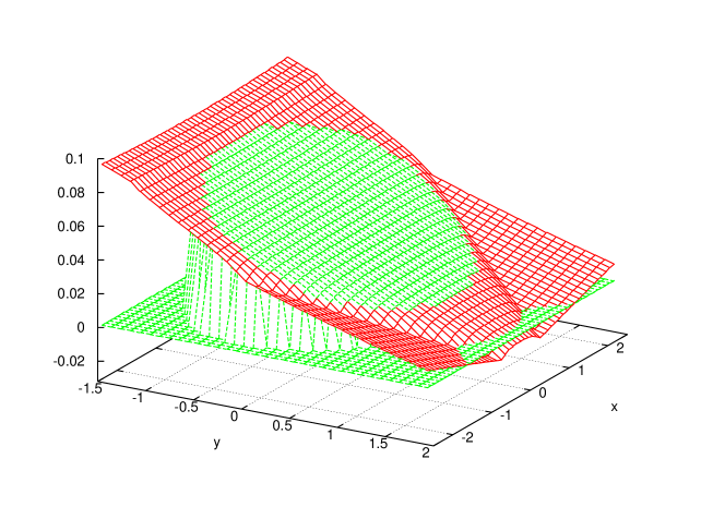
Figure 3: $\mathrm{Im}(A_{++-})$ as a function of $x$ and $y$ normalized to $-|A_{++-}(s_{0},s_{0},s_{0})|$. The curve with the plateau at zero indicates the phasespace. The thresholds in the various $\pi\pi$ channels are clearly visible.

5 Experimental Data and Fits

At the end of the seventies a review was written incorporating the then finished precision experiments on the charged kaon decays [18]. Since then there have been many new results on $K\to 3\pi$ decays. A recent attempt to refit the data using some of the partial numerics of [6] is [19]. We have in this paper recalculated the full expressions and will do a full fit to the data contrary to [19]. We analyze the data in terms of the widths given in Table 3. The numbers are taken from the review of particle properties [20]. We do not directly use the data for $\Gamma^{S}_{+-0}$ but instead fit directly to the measured quantity $\lambda$ as discussed below.

Decay	Width [GeV]	CHPT fit [GeV]
$K^{+}\to\pi^{+}\pi^{0}$	$(1.1245\pm 0.0078)\cdot 10^{-17}$	$1.124\cdot 10^{-17}$
$K_{S}\to\pi^{0}\pi^{0}$	$(2.3124\pm 0.0207)\cdot 10^{-15}$	$2.312\cdot 10^{-15}$
$K_{S}\to\pi^{+}\pi^{-}$	$(5.0543\pm 0.0211)\cdot 10^{-15}$	$5.054\cdot 10^{-15}$
$K_{L}\to\pi^{0}\pi^{0}\pi^{0}$	$(2.6901\pm 0.0402)\cdot 10^{-18}$	$2.655\cdot 10^{-18}$
$K_{L}\to\pi^{+}\pi^{-}\pi^{0}$	$(1.5978\pm 0.0283)\cdot 10^{-18}$	$1.626\cdot 10^{-18}$
$K_{S}\to\pi^{+}\pi^{-}\pi^{0}$	$(2.36\pm 0.81)\cdot 10^{-21}$	$3.1\cdot 10^{-21}$
$K^{+}\to\pi^{0}\pi^{0}\pi^{+}$	$(0.9194\pm 0.0426)\cdot 10^{-18}$	$0.911\cdot 10^{-18}$
$K^{+}\to\pi^{+}\pi^{+}\pi^{-}$	$(2.9706\pm 0.0272)\cdot 10^{-18}$	$2.973\cdot 10^{-18}$

Table 3: The various decay widths from the PDG tables[20].

In addition several slope parameters are measured in the various decays. The distributions in the Dalitz plot are conventionally described in terms of $x$ and $y$ defined in (22).

The decay amplitudes squared are now expanded as

$$\left|\frac{A(s_{1},s_{2},s_{3})}{A(s_{0},s_{0},s_{0})}\right|^{2}=1+gy+hy^{2}+kx^{2}$$ (44)

where we have used $CP$ invariance and the symmetries in the decays. For $K_{L}\to\pi^{0}\pi^{0}\pi^{0}$ $g=0$ and $k=h/3$. For $K_{S}\to\pi^{+}\pi^{-}\pi^{0}$ one defines the ratio $\lambda$ or measures directly the expansion of the amplitude [21]

$$\lambda = \frac{\displaystyle\int_{y_{min}}^{y_{max}}dy\int_{0}^{x_{lim}(y)}dxA^{L*}_{+-0}A^{S}_{+-0}}{\displaystyle\int_{y_{min}}^{y_{max}}dy\int_{0}^{x_{lim}(y)}dxA^{L*}_{+-0}A^{L}_{+-0}}$$

$$A^{S}_{+-0} = \gamma_{S}x-\xi_{S}xy\,.$$ (45)

The various measurements are given in Table 4. Experiments after 1980 have been cited explicitly. Earlier references can be found in the PDG[20] or in the comprehensive review [18]. Notice that there are significant discrepancies between the various experiments indicated by the fairly large scale factors.

Decay	Quantity		S	Ref.	CHPT fit
$K_{L}\to\pi^{0}\pi^{0}\pi^{0}$	$h$	$-0.0033\pm 0.0013$		[22]
	$h$	$-0.0061\pm 0.0010$		[23]
	$h$	$-0.00506\pm 0.00135$	1.7	average	$-$0.0072
$K_{L}\to\pi^{+}\pi^{-}\pi^{0}$	$g$	$0.678\pm 0.008$	1.5	[21, 20]	0.677
	$h$	$0.076\pm 0.006$		[21, 20]	0.085
	$k$	$0.0099\pm 0.0015$		[21, 20]	0.0055
$K_{S}\to\pi^{+}\pi^{-}\pi^{0}$	Re($\lambda$)	$0.0316\pm 0.0062$		[21, 24]	0.0359
	Im($\lambda$)	$-0.0088\pm 0.0068$		[21, 24]	$-$0.003
	$\gamma_{S}$	$(3.3\pm 0.5)\cdot 10^{-8}$		[21]	$3.4\cdot 10^{-8}$
	$\xi_{S}$	$(0.4\pm 0.8)\cdot 10^{-8}$		[21]	$-0.2\cdot 10^{-8}$
$K^{\pm}\to\pi^{0}\pi^{0}\pi^{\pm}$	$g$	$0.652\pm 0.031$	2.7	[25, 26, 20]	0.638
	$h$	$0.057\pm 0.018$	1.4	[25, 26, 20]	0.074
	$k$	$0.0197\pm 0.0054$		[25, 20]	0.0045
$K^{+}\to\pi^{+}\pi^{+}\pi^{-}$	$g$	$-0.2154\pm 0.0035$	1.4	[20]	$-$0.216
	$h$	$0.012\pm 0.008$	1.4	[20]	0.012
	$k$	$-0.0101\pm 0.0034$	2.1	[20]	$-$0.0052
$K^{-}\to\pi^{-}\pi^{-}\pi^{+}$	$g$	$-0.217\pm 0.007$	2.5	[20]
	$h$	$0.010\pm 0.006$		[20]
	$k$	$-0.0084\pm 0.0019$	2.1	[20]

Table 4: The measurements of the Dalitz plot distributions. Notice that in many cases the scale factors calculated with the PDG[20] method are sizable. The references refer to the most recent measurements and the PDG. S is the scale factor calculated using the prescription of [20].

The data have been analyzed previously in terms of expansions in $x$ and $y$ of the amplitudes.

$$A^{L}_{000} = 3(\alpha_{1}+\alpha_{3})+3(\zeta_{1}-2\zeta_{3})\left(y^{2}+\frac{1}{3}x^{2}\right)\,,$$

$$A^{L}_{+-0} = (\alpha_{1}+\alpha_{3})-(\beta_{1}+\beta_{3})y+(\zeta_{1}-2\zeta_{3})\left(y^{2}+\frac{1}{3}x^{2}\right)+(\xi_{1}-2\xi_{3})\left(y^{2}-\frac{1}{3}x^{2}\right)\,,$$

$$A^{S}_{+-0} = \frac{2}{3}\sqrt{3}\,\gamma_{3}x-\frac{4}{3}\xi_{3}^{\prime}xy\,,$$

$$A_{00+} = \left(-\alpha_{1}+\frac{1}{2}\alpha_{3}\right)+\left(\beta_{1}-\frac{1}{2}\beta_{3}-\sqrt{3}\gamma_{3}\right)y+(-\zeta_{1}-\zeta_{3})\left(y^{2}+\frac{1}{3}x^{2}\right)$$

$$+(-\xi_{1}-\xi_{3}-\xi_{3}^{\prime})\left(y^{2}-\frac{1}{3}x^{2}\right)\,,$$

$$A_{++-} = \left(-2\alpha_{1}+\alpha_{3}\right)+\left(-\beta_{1}+\frac{1}{2}\beta_{3}-\sqrt{3}\gamma_{3}\right)y+(-2\zeta_{1}-2\zeta_{3})\left(y^{2}+\frac{1}{3}x^{2}\right)$$ (46)

$$+(\xi_{1}+\xi_{3}-\xi_{3}^{\prime})\left(y^{2}-\frac{1}{3}x^{2}\right)\,.$$

A main problem in dealing with the data fitting is the question of how to deal with the isospin breaking effects. The phase-space itself is very sensitive to the precise masses of the pions and kaons which are used. There are several ways to deal with this problem. One is to first fit the expressions (5) to the data where $x$ and $y$ are defined with $s_{0}$ calculated with the physical masses but otherwise the charged pion mass as in (22). The result of this fit is shown in Table 5. Here we have assumed that the only complex phase appearing is the relative phase between $A_{0}$ and $A_{2}$. The errors quoted are the minuit errors. For the $K_{S}$-measurements only $\mbox{Re}(\lambda)$ is included. Leaving it out changes the $\chi^{2}/DOF$ to 3.9/4 but all parameters stay within the errors given.

quantity	Ref. [18]	Ref. [6]	Our fit	$p^{2}$	$\tilde{K}_{i}=0$
$|A_{0}|$	$0.4687\pm 0.0006$	$0.4699\pm 0.0012$	$0.4622\pm 0.0014$	input	input
$|A_{2}|$	$0.0210\pm 0.0001$	$0.0211\pm 0.0001$	$0.0212\pm 0.0001$	input	input
$\delta_{2}-\delta_{0}$	$(-45.6\pm 5)^{\rm o}$	$(-61.5\pm 4)^{\rm o}$	$(-58.2\pm 4)^{\rm o}$	—	—
$\alpha_{1}$	$91.4\pm 0.24$	$91.71\pm 0.32$	$93.16\pm 0.36$	74.0(73.5)	59.4
$\alpha_{3}$	$-7.14\pm 0.36$	$-7.36\pm 0.47$	$-6.72\pm 0.46$	$-4.8(4.8)$	$-6.5$
$\beta_{1}$	$-25.83\pm 0.41$	$-25.68\pm 0.27$	$-27.06\pm 0.43$	$-17.7(16.2)$	$-21.9$
$\beta_{3}$	$-2.48\pm 0.48$	$-2.43\pm 0.41$	$-2.22\pm 0.47$	$-1.2(1.1)$	$-1.0$
$g_{3}$	$2.51\pm 0.36$	$2.26\pm 0.23$	$2.95\pm 0.32$	$2.3(2.1)$	$2.5$
$\zeta_{1}$	$-0.37\pm 0.11$	$-0.47\pm 0.15$	$-0.40\pm 0.19$	—	0.26
$\zeta_{3}$	—	$-0.21\pm 0.08$	$-0.09\pm 0.10$	—	$-0.01$
$\xi_{1}$	$-1.25\pm 0.12$	$-1.51\pm 0.30$	$-1.83\pm 0.30$	—	$-0.46$
$\xi_{3}$	—	$-0.12\pm 0.17$	$-0.17\pm 0.16$	—	$-0.01$
$\xi_{3}^{\prime}$	—	$-0.21\pm 0.51$	$-0.56\pm 0.42$	—	$-0.06$
$\chi^{2}/DOF$	$12.8/3$	$10.3/2$	$5.4/5$	—	—

Table 5: The values of the parameters in the expansion in $x$ and $y$ of the $K\to 3\pi$ amplitudes and the $K\to\pi\pi$ amplitudes. The $\chi^{2}$ quoted are for the fits with the then used data. $|A_{0}|$ and $|A_{2}|$ are in units of $10^{-6}~{}GeV$. $\alpha_{1}$,…,$\xi_{3}^{\prime}$ are in units of $10^{-8}$.

In the column labeled $p^{2}$ in Table 5 we fixed $G_{8}$ and $G_{27}$ from the result for $A_{0}$ and $A_{2}$ at tree level and show the predictions for the linear slopes in the amplitude at this order. The source of the differences with [6] is not obvious but could be due to a different pion and kaon mass. The numbers in the table were calculated using the charged pion and kaon masses, using the neutral ones instead leads to the numbers in brackets. As can be seen a general reasonable agreement within about 40% is obtained. The input here determines $G_{8}=10.4$ and $G_{27}=0.61$ when we used for $F_{0}$ the pion decay constant $F_{\pi}$ and used $F_{\pi}$ and $F_{K}$ in the tree level amplitude with the physical values.

Going to the next order, we first show also in Table 5 in the column labeled $\tilde{K}_{i}=0$ the $p^{4}$ results with $G_{8}$ and $G_{27}$ fixed to fit $|A_{0}|$ and $|A_{2}|$. These were calculated with charged pion and kaon mass. The input here determines $G_{8}=5.47$ and $G_{27}=0.39$. The change compared to the previous is an indication of the size of the $p^{4}$ effect. It should be kept in mind that we have chosen to normalize the lowest order including one factor of $1/F_{K}$, changing that to $1/F_{\pi}$ changes the relative size of the $p^{2}$ and $p^{4}$ contributions significantly. There is as well a mild dependence on the value of the $L_{i}^{r}$ used. We use in general a scale of $\mu=0.77$ GeV and the $L_{i}^{r}$ values of the one-loop fit of [27], the $p^{4}$ fit including the latest $K_{\ell 4}$ data. These values are (all at $\mu=0.77$ GeV.)

$$\displaystyle L_{1}^{r}=0.38\cdot 10^{-3},\quad L_{2}^{r}=1.59\cdot 10^{-3},\quad L_{3}^{r}=-2.91\cdot 10^{-3},\quad L_{4}^{r}=0,$$

$$\displaystyle L_{5}^{r}=1.46\cdot 10^{-3},\quad L_{6}^{r}=0,\quad L_{7}^{r}=-0.49\cdot 10^{-3},\quad L_{8}^{r}=1.0\cdot 10^{-3}\,.$$ (47)

It is not possible to determine all 13 quantities $G_{8}$, $G_{27}$ and $\tilde{K}_{1}$,…,$\tilde{K}_{11}$. In principle it cannot be done if we try to fit to the 12 quantities listed in Table 5, but in practice the situation is even worse, simply fitting the possible parameters without constraints leads to fits with negligible tree level contributions. We have therefore chosen a two-step process, first we study the variation of fitting subsets of $G_{8}$, $G_{27}$ and $\tilde{K}_{1}$,…,$\tilde{K}_{11}$ to $|A_{0}|$,…,$\xi_{3}^{\prime}$. This allows for a more direct study of the various dependencies on parameters. Finally we present the direct fit where we compare directly to the data, but allowing in addition for a variable phase $\delta_{2}-\delta_{0}$ between $A_{0}$ and $A_{2}$

The various relations advocated in [7] follow if one sets

$$\tilde{K}_{1}=\tilde{K}_{4}=0\quad\mbox{and}\quad\tilde{K}_{8}=\cdots=\tilde{K}_{11}=0\,.$$ (48)

The resulting fit values are in Table 6, column 2. Several of the $\tilde{K}_{i}$ are uncomfortably large but inspection of the size of the $p^{2}$ versus $p^{4}$ contributions shows nothing conspicuous. The source of the problem turned out to be $\gamma_{3}$ which with the constraints of Eq. (48) can only be fitted by varying $\tilde{K}_{6}$ but it comes multiplied with a small factor. It then produces fairly large other $\tilde{K}_{i}$ in order to minimize the effect of $\tilde{K}_{7}$ on the other quantities. We have therefore also fitted using the constraints

$$\tilde{K}_{1}=\tilde{K}_{4}=\tilde{K}_{6}=0\quad\mbox{and}\quad\tilde{K}_{8}=\cdots=\tilde{K}_{11}=0\,.$$ (49)

We can now attempt to also determine somewhat the combinations $\tilde{K}_{1}$ and $\tilde{K}_{4}$. Leaving $\tilde{K}_{1}$ free hardly changes the quality of the fit but shows that the actual value of $G_{8}$ can change over a fairly wide range. The results are shown in the fourth column of Table 6 with constraints

$$\tilde{K}_{4}=0\quad\mbox{and}\quad\tilde{K}_{8}=\cdots=\tilde{K}_{11}=0\,.$$ (50)

The same type of correlation occurs for $G_{27}$ and $\tilde{K}_{4}$ as shown with the results in column 5 of the Table where we fitted with constraints

$$\tilde{K}_{1}=0,\quad\tilde{K}_{4}=0.1\quad\mbox{and}\quad\tilde{K}_{8}=\cdots=\tilde{K}_{11}=0\,.$$ (51)

The reason we have picked a fixed value for $\tilde{K}_{4}$ is because there is very long, narrow and extremely shallow fitting region that moves in the end to a very small $G_{27}$ and values for $\tilde{K}_{4}$, $\tilde{K}_{5}$, $\tilde{K}_{6}$ and $\tilde{K}_{7}$ that are simply enormous but a total $\chi^{2}$ which is only marginally smaller than the one shown, 11.7 rather than 11.9.

constraints	Eq. (48)	Eq. (49)	Eq. (50)	Eq. (51)	Eq. (48)
Fitted	$|A_{0}|,\ldots,\xi_{3}^{\prime}$				experiment
$G_{8}$	5.47(2)	5.47(2)	7.24(2.04)	5.49	5.45(2)
$G_{27}$	0.392(2)	0.392(2)	0.392(2)	0.139	0.392(2)
$10^{3}\tilde{K}_{1}/G_{8}$	$\equiv 0$	$\equiv 0$	$-$8.5(7.5)	$\equiv 0$	$\equiv 0$
$10^{3}\tilde{K}_{2}/G_{8}$	54.7(2.8)	53.6(2.7)	41.3(11.4)	53.7	51.9(3.2)
$10^{3}\tilde{K}_{3}/G_{8}$	3.0(1.4)	3.5(1.3)	10.0(6.3)	3.2	3.8(1.5)
$10^{3}\tilde{K}_{4}/G_{27}$	$\equiv 0$	$\equiv 0$	$\equiv 0$	$\equiv 100$	$\equiv 0$
$10^{3}\tilde{K}_{5}/G_{27}$	$-$54.5(23.4)	$-$19.8(9.6)	$-$54.5(23.1)	$-$49.4	$-$42.5(16.6)
$10^{3}\tilde{K}_{6}/G_{27}$	$-$185(114)	$\equiv 0$	$-$184(113)	$-$366	$-$166(113)
$10^{3}\tilde{K}_{7}/G_{27}$	114(46)	45.1(18.2)	114(46)	199	120(32)
$\chi^{2}/DOF$	12.3/5	14.9/6	11.8/4	11.9/4	26.8/10

Table 6: The results for $G_{8}$, $G_{27}$ and the $\tilde{K}_{i}$ for the various constraints discussed in the text. In brackets are the MINUIT errors.

How well do the relations proposed in [7] stand up to the new data. In practice, for the octet which dominates the $\Delta I=1/2$ part, it means that $\alpha_{1}$ determines $\zeta_{1}$, $\beta_{1}$ determines $\xi_{1}$. The first of these relations is extremely well satisfied, but it is hard to get $\xi_{1}$ to better than about 2.5 standard deviations, the value obtained from the various above fits is

$$\xi_{1}\approx(-0.98-i0.13)\cdot 10^{-8}\,.$$ (52)

Inspection of the numerical coefficients for the octet parameters that only contribute suppressed by powers of $m_{\pi}^{2}$ reveals that some of them show up with large numerical coefficients. One can then instead choose to leave $K_{8}$ or $\tilde{K}_{9}$ free rather than $\tilde{K}_{1}$. The resulting fits are of similar quality to the one with $\tilde{K}_{1}$ free and do not significantly improve the prediction for $\xi_{1}$ given in (52). The possible variation is less than 10%.

There is no similar single value with significant discrepancies for the $\Delta I=3/2$ parameters. The above named problem with $\gamma_{3}$ does not lead to a major discrepancy but typically the quadratic quantities are the ones with a deviation of about 0.5 to 1.4 $\sigma$.

Varying the masses of the pion and kaon or the eta mass used in the loops does not change the results of the fits significantly.

The fit via the intermediate step of $|A_{0}|,\ldots,\xi_{3}^{\prime}$ is fairly fast and allows an easy study of the variation with the inputs. We have also done the fit directly to all the experimental data listed in Tables 3 and 4 with only the use of Re($\lambda$) for the $K_{S}\to\pi^{+}\pi^{-}\pi^{0}$ data. The masses used in the phase space were the physical masses occurring in the decays. The masses used in the amplitudes are the physical kaon mass and the pion mass such that $3m_{\pi}^{2}=\sum_{i=1,3}m_{\pi^{i}}^{2}$ is satisfied. The eta mass in the loops we then calculated using the GMO relation. The resulting values for the $\tilde{K}_{i}$ are given in the last column of Table 6 and the values for the widths and Dalitz plot distribution variables are in the column labeled CHPT fit in Tables 3 and 4. We have allowed an extra phase between $A_{0}$ and $A_{2}$ in this fit. Otherwise this fit corresponds to the constraints (48). The higher $\chi^{2}$ is mainly due to the fact that $\xi_{1}$ has been fitted to more than one quantity, and here we have the discrepancy with the slope $k$ in $K_{L}\to\pi^{+}\pi^{-}\pi^{0}$ and $K^{+}\to\pi^{0}\pi^{0}\pi^{+}$. These together account for 16.4 of $\chi^{2}$.

The fact that the last fit and the fit via the intermediate step of $|A_{0}|,\ldots,\xi_{3}^{\prime}$ agree very well is an indication that the isospin breaking effects at the amplitude level are small. An estimate can be done by calculating the amplitudes and the slopes with the masses of ${K^{0}}$, ${\pi^{0}}$ and comparing them with the amplitudes calculated with $m_{K^{+}}$, $m_{\pi^{+}}$. Since often factors of $m_{K}^{2}-m_{\pi}^{2}$ appear this is the worst case. The changes are typically 2% for the amplitudes, 5-8% for the linear slopes and up to 20% for the quadratic slopes.

6 Conclusions

In this paper we have recalculated the $K\to\pi\pi$ and $K\to\pi\pi\pi$ amplitudes to next-to-leading order in CHPT in the isospin limit and presented the amplitudes in a simple form suitable for dispersive estimates of higher orders.

We have performed a new global fit to all available kaon data at this level taking into account the isospin breaking in the phase space. Work is under progress to include isospin breaking also in the amplitudes.

At present the situation is that a satisfactory agreement is obtained with the predictions keeping in mind that for the quadratic slopes higher order corrections could be sizable as happened with the analogous results in $\eta\to 3\pi$ results. A discussion of the latter together with references can be found in [28]. Some work exists on dispersive corrections in $K\to 3\pi$ [17], but more study is needed to fit their results in this framework.

Now the isospin breaking corrections, including possible electromagnetic radiative corrections, need to be studied to see if they are the cause of the differences in the quadratic Dalitz plot parameters. Work exists to a large extent for the $K\to 2\pi$ decays [29], but little has been done using modern methods for $K\to 3\pi$ decays.

Appendix A Ambiguity in the definition of $M_{i}$

The functions $M_{i}(s)$ defined in Eq. (3) are not unique for two reasons. The variables $s_{1},s_{2}$ and $s_{3}$ are not independent, they satisfy the relation (22), and low powers of $s_{1},s_{2}$ and $s_{3}$ can be fitted in more than one of the $M_{i}$ functions.

As a simple example, we could have added

$$\delta M_{0}(s)=\alpha\left(s-s_{0}\right)\,,$$ (A.1)

with $\alpha$ any constant, without changing the result, for $A^{L}_{000}$. The full set of these ambiguities can be derived by checking the total number of independent terms that exist in the polynomial expansion of the amplitudes and comparing it with the the same expansion of the $M_{i}(s)$.

The changes of the functions that leave all amplitudes unchanged are

$$M_{0}(s) \longrightarrow M_{0}(s)+\delta_{1}\left(s-s_{0}\right)$$ (A.2)

$$M_{1}(s) \longrightarrow M_{1}(s)+\delta_{2},\quad M_{2}(s)\longrightarrow M_{2}(s)-\frac{1}{2}\delta_{2}\,;$$ (A.3)

$$M_{1}(s) \longrightarrow M_{1}(s)+\delta_{3}\left(s-s_{0})\right),\quad M_{2}(s)\longrightarrow M_{2}(s)+\delta_{3}\left(s-s_{0})\right)\,;$$ (A.4)

$$M_{1}(s) \longrightarrow M_{1}(s)+2\delta_{4}s,\quad M_{2}(s)\longrightarrow M_{2}(s)-\delta_{4}s,\quad M_{3}(s)\longrightarrow M_{3}(s)+\delta_{4}\,;$$ (A.5)

$$M_{1}(s) \longrightarrow M_{1}(s)-2\delta_{5}s\left(s-3s_{0}\right),\quad M_{2}(s)\longrightarrow M_{2}(s)+\delta_{5}s\left(s-3s_{0}\right),$$

$$M_{3}(s) \longrightarrow M_{3}(s)+\delta_{5}s\,;$$ (A.6)

$$M_{1}(s) \longrightarrow M_{1}(s)+\frac{2}{3}\delta_{6}\left(s-3s_{0}\right)^{3},\quad M_{2}(s)\longrightarrow M_{2}(s)-\frac{1}{3}\delta_{6}s^{2}\left(s-9s_{0}\right),$$

$$M_{3}(s) \longrightarrow M_{3}(s)+\delta_{6}s^{2}\,;$$ (A.7)

$$M_{4}(s) \longrightarrow M_{4}(s)+\delta_{7}\,;$$ (A.8)

$$M_{4}(s) \longrightarrow M_{4}(s)+\delta_{8}s\,,\quad M_{5}(s)\longrightarrow M_{5}(s)+\delta_{8};$$ (A.9)

$$M_{5}(s) \longrightarrow M_{5}(s)+\delta_{9},\quad M_{6}(s)\longrightarrow M_{5}(s)+\delta_{9};$$ (A.10)

$$M_{4}(s) \longrightarrow M_{4}(s)-\delta_{10}s\left(s-3s_{0}\right)\,,\quad M_{5}(s)\longrightarrow M_{5}(s)+\delta_{10}s;$$ (A.11)

$$M_{5}(s) \longrightarrow M_{5}(s)+\delta_{11}s,\quad M_{6}(s)\longrightarrow M_{5}(s)+\delta_{11}s;$$ (A.12)

$$M_{4}(s) \longrightarrow M_{4}(s)+\delta_{12}\left(s^{3}-9s_{0}s^{2}+18s_{0}^{2}s\right),\quad M_{5}(s)\longrightarrow M_{5}(s)+\delta_{12}s^{2};$$

$$M_{6}(s) \longrightarrow M_{6}(s)-2\delta_{12}s^{2};$$ (A.13)

$$M_{4}(s) \longrightarrow M_{4}(s)+\delta_{13}3s_{0}\left(s^{3}-9s_{0}s^{2}+18s_{0}^{2}s\right),\quad M_{5}(s)\longrightarrow M_{5}(s)+\delta_{13}s^{3},$$

$$M_{6}(s) \longrightarrow M_{6}(s)-2\delta_{13}\left(s^{2}-9s_{0}s^{2}\right)\,.$$ (A.14)

The triplets $(M_{7},M_{8},M_{9})$ and $(M_{10},M_{11},M_{12})$ have an ambiguity similar to (A.3)-(A), leading to a total ambiguity of 23 free parameters.

Appendix B Explicit expressions for the $M_{i}(s)$ in $K\to 3\pi$.

We write the $M_{i}(s)$ functions defined in Eq. (3) as

$$M_{i}(s)=\left.M_{i}(s)\right|_{p^{2}}+i\frac{CF_{0}^{4}}{F_{\pi}^{3}F_{K}}\left\{\frac{G_{8}}{F_{\pi}^{2}}M_{i}^{8}(s)+\frac{G_{8}^{\prime}}{F_{\pi}^{2}}M_{i}^{8\prime}(s)+\frac{G_{27}}{F_{\pi}^{2}}M_{i}^{27}(s)\right\}\,.$$ (B.1)

The effect of $G_{8}^{\prime}$ cannot be distinguished from higher order coefficients in decays not involving external fields. This was known at tree level earlier and has been proven to one-loop in [5]. The effect of $M_{i}^{8\prime}(s)$ can be reconstructed from $M_{i}^{8}(s)$ by the changes

$$N_{10}^{r}+2N_{11}^{r}+N_{12}^{r} \longrightarrow N_{10}^{r}+2N_{11}^{r}+N_{12}^{r}+\frac{G_{8}^{\prime}}{G_{8}}\left(2L_{5}^{r}-16L_{6}^{r}-8L_{8}^{r}\right)\,,$$

$$N_{7}^{r} \longrightarrow N_{7}^{r}+\frac{G_{8}^{\prime}}{G_{8}}\left(-4L_{4}^{r}\right)\,.$$ (B.2)

The results for the $K\to\pi\pi$ amplitudes are in full agreement with [14] and can be found there.

We have brought the $M_{i}^{j}(s)$ in a form that satisfies the isospin relations (3). These can be used in the form

$$M_{1}^{j}(s) = M_{0}^{j}(s)-2M_{2}^{j}(s)\,,$$

$$M_{6}^{j}(s) = M_{5}^{j}(s)-M_{9}^{j}(s)-M_{12}^{j}(s)\,,$$

$$M_{7}^{j}(s) = 2M_{4}^{j}(s)-\frac{1}{2}M_{10}^{j}(s)+M_{11}^{j}(s)\,,$$

$$M_{8}^{j}(s) = -M_{4}^{j}(s)+\frac{1}{2}M_{10}^{j}(s)$$ (B.3)

to reconstruct these. We have extensively used the GMO relation in writing them in this form.

The explicit expressions for $\overline{A}$, $\overline{B}$ and $\overline{B}_{1}$, the finite part of the loop functions, can be found in many places, e.g. [30].

The octet ones are:

$$M^{8}_{0}(s)=$$ (B.4)

$$+(N_{1}^{r}+N_{2}^{r})\,(-2\,m_{\pi}^{2}\,m_{K}^{2}+3\,m_{\pi}^{2}\,s-2\,m_{\pi}^{4}+m_{K}^{2}\,s-s^{2})$$

$$+N_{3}^{r}\,(2\,m_{\pi}^{2}\,m_{K}^{2}-3\,m_{\pi}^{2}\,s+5\,m_{\pi}^{4}-m_{K}^{2}\,s+m_{K}^{4}-2\,s^{2})$$

$$+N_{5}^{r}\,(2\,m_{\pi}^{2}\,m_{K}^{2}-2\,m_{\pi}^{2}\,s+2\,m_{\pi}^{4}+2\,m_{K}^{2}\,s)+N_{7}^{r}\,(8\,m_{\pi}^{2}\,m_{K}^{2}-4\,m_{K}^{2}\,s)$$

$$+N_{8}^{r}\,(-2\,m_{\pi}^{2}\,s+2\,m_{\pi}^{4}+4\,m_{K}^{2}\,s)+N_{9}^{r}\,(-2\,m_{\pi}^{2}\,m_{K}^{2}-2\,m_{\pi}^{2}\,s+2\,m_{\pi}^{4}+2\,m_{K}^{2}\,s)$$

$$+(N_{10}^{r}+2N_{11}^{r}+N_{12}^{r})\,(-4\,m_{\pi}^{2}\,m_{K}^{2})$$

$$+L_{1}^{r}\,(32\,m_{\pi}^{2}\,m_{K}^{2}-48\,m_{\pi}^{2}\,s+32\,m_{\pi}^{4}-16\,m_{K}^{2}\,s+16\,s^{2})$$

$$+L_{2}^{r}\,(-16\,m_{\pi}^{2}\,m_{K}^{2}+24\,m_{\pi}^{2}\,s-40\,m_{\pi}^{4}+8\,m_{K}^{2}\,s-8\,m_{K}^{4}+16\,s^{2})$$

$$+L_{3}^{r}\,(16\,m_{\pi}^{2}\,m_{K}^{2}-24\,m_{\pi}^{2}\,s+16\,m_{\pi}^{4}-8\,m_{K}^{2}\,s+8\,s^{2})$$

$$+L_{4}^{r}\,(-16\,m_{\pi}^{2}\,m_{K}^{2}+16\,m_{\pi}^{2}\,s-16\,m_{\pi}^{4})+L_{5}^{r}\,(-8\,m_{\pi}^{2}\,m_{K}^{2}+16\,m_{\pi}^{2}\,s-16\,m_{\pi}^{4})$$

$$+({1}/{(16\pi^{2})})\,(4/3\,m_{\pi}^{2}\,m_{K}^{2}+1/2\,m_{\pi}^{2}\,s-1/2\,m_{\pi}^{4}-3/2\,m_{K}^{2}\,s+1/2\,m_{K}^{4})$$

$$+\overline{A}(m_{\pi}^{2})\,(-19/8\,m_{\pi}^{2}-2/3\,m_{K}^{2}+21/8\,s)+\overline{A}(m_{K}^{2})\,(-13/4\,m_{\pi}^{2}-1/3\,m_{K}^{2}+3\,s)$$

$$+\overline{A}(m_{\eta}^{2})\,(-3/8\,m_{\pi}^{2}+3/8\,s)+\overline{B}(m_{\pi}^{2},m_{\pi}^{2},s)\,(1/2\,m_{\pi}^{2}\,m_{K}^{2}-2\,m_{\pi}^{2}\,s+m_{\pi}^{4}+s^{2})$$

$$+\overline{B}(m_{\pi}^{2},m_{K}^{2},s)\,(13/8\,m_{\pi}^{2}\,m_{K}^{2}-5/4\,m_{\pi}^{2}\,s-5/8\,m_{K}^{2}\,s-1/8\,m_{K}^{4}+3/4\,s^{2})$$

$$+\overline{B}(m_{K}^{2},m_{K}^{2},s)\,(1/4\,m_{\pi}^{2}\,s+1/4\,m_{K}^{2}\,s-1/4\,s^{2})$$

$$+\overline{B}(m_{\eta}^{2},m_{K}^{2},s)\,(-5/24\,m_{\pi}^{2}\,m_{K}^{2}+1/8\,m_{K}^{2}\,s+1/24\,m_{K}^{4})+\overline{B}(m_{\eta}^{2},m_{\eta}^{2},s)\,(1/18\,m_{\pi}^{2}\,m_{K}^{2})$$

$$+\overline{B_{1}}(m_{\pi}^{2},m_{K}^{2},s)\,(-3/4\,m_{\pi}^{2}\,m_{K}^{2}+1/2\,m_{\pi}^{4}+1/4\,m_{K}^{4})$$

$$+\overline{B_{1}}(m_{\eta}^{2},m_{K}^{2},s)\,(1/4\,m_{\pi}^{2}\,m_{K}^{2}-1/4\,m_{K}^{4})\,.$$

$$M^{8}_{2}(s)=$$

$$+N_{3}^{r}\,(-s^{2})+L_{2}^{r}\,(8\,s^{2})+({1}/{(16\pi^{2})})\,(1/6\,s^{2})$$

$$+\overline{B}(m_{\pi}^{2},m_{\pi}^{2},s)\,(1/2\,m_{\pi}^{2}\,m_{K}^{2}-3/4\,m_{\pi}^{2}\,s+1/2\,m_{\pi}^{4}-1/4\,m_{K}^{2}\,s+1/4\,s^{2})$$

$$+\overline{B}(m_{\pi}^{2},m_{K}^{2},s)\,(1/2\,m_{\pi}^{2}\,m_{K}^{2}-1/2\,m_{\pi}^{2}\,s+1/4\,m_{\pi}^{4}-1/2\,m_{K}^{2}\,s+1/4\,m_{K}^{4}+1/4\,s^{2}).$$

$$M^{8}_{3}(s)=$$ (B.6)

$$+\overline{B}(m_{\pi}^{2},m_{\pi}^{2},s)\,(1/3\,m_{\pi}^{2}-1/12\,s)+\overline{B}(m_{\pi}^{2},m_{K}^{2},s)\,(1/8\,m_{\pi}^{2}+1/24\,m_{K}^{2}-1/24\,s)$$

$$+\overline{B}(m_{\eta}^{2},m_{K}^{2},s)\,(-1/8\,m_{\pi}^{2}+5/8\,m_{K}^{2}-1/8\,s)+\overline{B_{1}}(m_{\pi}^{2},m_{K}^{2},s)\,(-1/12\,m_{\pi}^{2}+1/12\,m_{K}^{2})$$

$$+\overline{B_{1}}(m_{\eta}^{2},m_{K}^{2},s)\,(1/12\,m_{\pi}^{2}-1/12\,m_{K}^{2}).$$

$$M^{8}_{4}(s) = 0.$$ (B.7)

$$M^{8}_{5}(s)=$$ (B.8)

$$+\overline{B}(m_{\pi}^{2},m_{K}^{2},s)\,(-1/8\,m_{\pi}^{2}-1/24\,m_{K}^{2}+1/24\,s)+\overline{B}(m_{K}^{2},m_{K}^{2},s)\,(-1/3\,m_{K}^{2}+1/12\,s)$$

$$+\overline{B}(m_{\eta}^{2},m_{K}^{2},s)\,(1/8\,m_{\pi}^{2}-5/8\,m_{K}^{2}+1/8\,s)+\overline{B_{1}}(m_{\pi}^{2},m_{K}^{2},s)\,(1/12\,m_{\pi}^{2}-1/12\,m_{K}^{2})$$

$$+\overline{B_{1}}(m_{\eta}^{2},m_{K}^{2},s)\,(-1/12\,m_{\pi}^{2}+1/12\,m_{K}^{2});$$

$$M^{8}_{9}(s) = -M^{8}_{3}(s).$$ (B.9)

$$M^{8}_{10}(s)=$$ (B.10)

$$+(N_{1}^{r}+N_{2}^{r})\,(-2\,m_{\pi}^{2}\,m_{K}^{2}+3\,m_{\pi}^{2}\,s-5\,m_{\pi}^{4}+m_{K}^{2}\,s-m_{K}^{4})$$

$$+N_{3}^{r}\,(2\,m_{\pi}^{2}\,m_{K}^{2}-3\,m_{\pi}^{2}\,s-m_{\pi}^{4}-m_{K}^{2}\,s-m_{K}^{4}+2\,s^{2})$$

$$+N_{5}^{r}\,(-8\,m_{\pi}^{2}\,m_{K}^{2}-2\,m_{\pi}^{2}\,s+2\,m_{\pi}^{4}+2\,m_{K}^{2}\,s-2\,m_{K}^{4})$$

$$+N_{7}^{r}\,(-4\,m_{\pi}^{2}\,m_{K}^{2}-4\,m_{K}^{2}\,s+4\,m_{K}^{4})$$

$$+N_{8}^{r}\,(-10\,m_{\pi}^{2}\,m_{K}^{2}-2\,m_{\pi}^{2}\,s+2\,m_{\pi}^{4}+4\,m_{K}^{2}\,s-4\,m_{K}^{4})$$

$$+N_{9}^{r}\,(-2\,m_{\pi}^{2}\,s+2\,m_{\pi}^{4}+2\,m_{K}^{2}\,s-2\,m_{K}^{4})+(N_{10}^{r}+2N_{11}^{r}+N_{12}^{r})\,(8\,m_{\pi}^{2}\,m_{K}^{2})$$

$$+L_{1}^{r}\,(32\,m_{\pi}^{2}\,m_{K}^{2}-48\,m_{\pi}^{2}\,s+80\,m_{\pi}^{4}-16\,m_{K}^{2}\,s+16\,m_{K}^{4})$$

$$+L_{2}^{r}\,(-16\,m_{\pi}^{2}\,m_{K}^{2}+24\,m_{\pi}^{2}\,s+8\,m_{\pi}^{4}+8\,m_{K}^{2}\,s+8\,m_{K}^{4}-16\,s^{2})$$

$$+L_{3}^{r}\,(16\,m_{\pi}^{2}\,m_{K}^{2}-24\,m_{\pi}^{2}\,s+40\,m_{\pi}^{4}-8\,m_{K}^{2}\,s+8\,m_{K}^{4})$$

$$+L_{4}^{r}\,(16\,m_{\pi}^{2}\,m_{K}^{2}+16\,m_{\pi}^{2}\,s-16\,m_{\pi}^{4})+L_{5}^{r}\,(16\,m_{\pi}^{2}\,s-16\,m_{\pi}^{4})$$

$$+({1}/{(16\pi^{2})})\,(11/9\,m_{\pi}^{2}\,m_{K}^{2}+4/9\,m_{\pi}^{2}\,s-1/3\,m_{\pi}^{4}-13/9\,m_{K}^{2}\,s+4/9\,m_{K}^{4}-1/3\,s^{2})$$

$$+\overline{A}(m_{\pi}^{2})\,(-25/8\,m_{\pi}^{2}-31/24\,m_{K}^{2}+21/8\,s)+\overline{A}(m_{K}^{2})\,(-5/2\,m_{\pi}^{2}-7/3\,m_{K}^{2}+3\,s)$$

$$+\overline{A}(m_{\eta}^{2})\,(-3/8\,m_{\pi}^{2}-3/8\,m_{K}^{2}+3/8\,s)$$

$$+\overline{B}(m_{\pi}^{2},m_{\pi}^{2},s)\,(-m_{\pi}^{2}\,m_{K}^{2}+3/2\,m_{\pi}^{2}\,s-m_{\pi}^{4}+1/2\,m_{K}^{2}\,s-1/2\,s^{2})$$

$$+\overline{B}(m_{\pi}^{2},m_{K}^{2},s)\,(-m_{\pi}^{2}\,m_{K}^{2}+m_{\pi}^{2}\,s-1/2\,m_{\pi}^{4}+m_{K}^{2}\,s-1/2\,m_{K}^{4}-1/2\,s^{2}).$$

$$M^{8}_{11}(s)=$$ (B.11)

$$+(N_{1}^{r}+N_{2}^{r}+N_{3}^{r}-16L_{1}^{r}-8L_{2}^{r}-8L_{3}^{r})\,(s^{2})$$

$$+({1}/{(16\pi^{2})})\,(-1/18\,m_{\pi}^{2}\,s+1/18\,m_{K}^{2}\,s+1/6\,s^{2})$$

$$+\overline{B}(m_{\pi}^{2},m_{\pi}^{2},s)\,(5/4\,m_{\pi}^{2}\,s-1/2\,m_{\pi}^{4}-1/4\,m_{K}^{2}\,s-3/4\,s^{2})$$

$$+\overline{B}(m_{\pi}^{2},m_{K}^{2},s)\,(-9/8\,m_{\pi}^{2}\,m_{K}^{2}+3/4\,m_{\pi}^{2}\,s+1/4\,m_{\pi}^{4}+1/8\,m_{K}^{2}\,s+3/8\,m_{K}^{4}-1/2\,s^{2})$$

$$+\overline{B}(m_{K}^{2},m_{K}^{2},s)\,(-1/4\,m_{\pi}^{2}\,s-1/4\,m_{K}^{2}\,s+1/4\,s^{2})$$

$$+\overline{B}(m_{\eta}^{2},m_{K}^{2},s)\,(5/24\,m_{\pi}^{2}\,m_{K}^{2}-1/8\,m_{K}^{2}\,s-1/24\,m_{K}^{4})+\overline{B}(m_{\eta}^{2},m_{\eta}^{2},s)\,(-1/18\,m_{\pi}^{2}\,m_{K}^{2})$$

$$+\overline{B_{1}}(m_{\pi}^{2},m_{K}^{2},s)\,(3/4\,m_{\pi}^{2}\,m_{K}^{2}-1/2\,m_{\pi}^{4}-1/4\,m_{K}^{4})$$

$$+\overline{B_{1}}(m_{\eta}^{2},m_{K}^{2},s)\,(-1/4\,m_{\pi}^{2}\,m_{K}^{2}+1/4\,m_{K}^{4}).$$

$$M^{8}_{12}(s) = M^{8}_{3}(s)=-M^{8}_{9}(s).$$ (B.12)

The 27 plet ones depend as well on the quantity

$$P_{K\pi}=\frac{1}{m_{K}^{2}-m_{\pi}^{2}}\,.$$ (B.13)

$$M^{27}_{0}(s)=$$ (B.14)

$$+D_{1}^{r}\,(-4/3\,m_{\pi}^{2}\,m_{K}^{2})$$

$$+D_{2}^{r}\,((2/3\,m_{\pi}^{2}\,m_{K}^{2}+10\,m_{\pi}^{2}\,s-40/3\,m_{\pi}^{4})+P_{K\pi}(10\,m_{\pi}^{4}\,s-40/3\,m_{\pi}^{6}))$$

$$+D_{4}^{r}\,((-11/2\,m_{\pi}^{2}\,m_{K}^{2}+m_{\pi}^{2}\,s+7/3\,m_{\pi}^{4}+3/2\,m_{K}^{2}\,s-5/6\,m_{K}^{4})$$

$$~{}~{}+P_{K\pi}\,(-10\,m_{\pi}^{4}\,s+40/3\,m_{\pi}^{6}))$$

$$+D_{5}^{r}\,(29/6\,m_{\pi}^{2}\,m_{K}^{2}-11\,m_{\pi}^{2}\,s+11\,m_{\pi}^{4}-3/2\,m_{K}^{2}\,s+5/6\,m_{K}^{4})$$

$$+D_{6}^{r}\,(5/3\,m_{\pi}^{2}\,m_{K}^{2}+1/3\,m_{\pi}^{2}\,s-1/3\,m_{\pi}^{4}-m_{K}^{2}\,s)$$

$$+D_{7}^{r}\,((-25/3\,m_{\pi}^{2}\,m_{K}^{2}-3\,m_{\pi}^{2}\,s+8\,m_{\pi}^{4}+6\,m_{K}^{2}\,s-10/3\,m_{K}^{4})$$

$$~{}~{}+P_{K\pi}\,D_{7}^{r}\,(-15\,m_{\pi}^{4}\,s+20\,m_{\pi}^{6}))$$

$$+D_{26}^{r}\,(-2/3\,m_{\pi}^{2}\,m_{K}^{2}+m_{\pi}^{2}\,s-2/3\,m_{\pi}^{4}+1/3\,m_{K}^{2}\,s-1/3\,s^{2})$$

$$+D_{27}^{r}\,(4/3\,m_{\pi}^{2}\,m_{K}^{2}-2\,m_{\pi}^{2}\,s+10/3\,m_{\pi}^{4}-2/3\,m_{K}^{2}\,s+2/3\,m_{K}^{4}-4/3\,s^{2})$$

$$+D_{28}^{r}\,(8\,m_{\pi}^{2}\,m_{K}^{2}-12\,m_{\pi}^{2}\,s+12\,m_{\pi}^{4}-4\,m_{K}^{2}\,s+4/3\,m_{K}^{4})$$

$$+D_{29}^{r}\,(-3/2\,m_{\pi}^{2}\,m_{K}^{2}+9/4\,m_{\pi}^{2}\,s-13/4\,m_{\pi}^{4}+3/4\,m_{K}^{2}\,s-7/12\,m_{K}^{4}+s^{2})$$

$$+D_{30}^{r}\,(3/2\,m_{\pi}^{2}\,m_{K}^{2}-9/4\,m_{\pi}^{2}\,s+1/4\,m_{\pi}^{4}-3/4\,m_{K}^{2}\,s-5/12\,m_{K}^{4}+2\,s^{2})$$

$$+D_{31}^{r}\,(4\,m_{\pi}^{2}\,m_{K}^{2}-6\,m_{\pi}^{2}\,s+4\,m_{\pi}^{4}-2\,m_{K}^{2}\,s+2\,s^{2})$$

$$+L_{1}^{r}\,(-32\,m_{\pi}^{2}\,m_{K}^{2}+48\,m_{\pi}^{2}\,s-32\,m_{\pi}^{4}+16\,m_{K}^{2}\,s-16\,s^{2})$$

$$+L_{2}^{r}\,(16\,m_{\pi}^{2}\,m_{K}^{2}-24\,m_{\pi}^{2}\,s+40\,m_{\pi}^{4}-8\,m_{K}^{2}\,s+8\,m_{K}^{4}-16\,s^{2})$$

$$+L_{3}^{r}\,((-58/3\,m_{\pi}^{2}\,m_{K}^{2}+34\,m_{\pi}^{2}\,s-118/3\,m_{\pi}^{4}+8\,m_{K}^{2}\,s-8\,s^{2})$$

$$~{}~{}+P_{K\pi}\,(40\,m_{\pi}^{4}\,s-160/3\,m_{\pi}^{6}))$$

$$+L_{4}^{r}\,(16\,m_{\pi}^{2}\,m_{K}^{2}-16\,m_{\pi}^{2}\,s+16\,m_{\pi}^{4})$$

$$+L_{5}^{r}\,((8\,m_{\pi}^{2}\,m_{K}^{2}-16\,m_{\pi}^{2}\,s+68/3\,m_{\pi}^{4})+P_{K\pi}\,(-20\,m_{\pi}^{4}\,s+80/3\,m_{\pi}^{6}))$$

$$+({1}/{(16\pi^{2})})\,((503/324\,m_{\pi}^{2}\,m_{K}^{2}+197/216\,m_{\pi}^{2}\,s-287/216\,m_{\pi}^{4}-401/216\,m_{K}^{2}\,s$$

$$~{}~{}+401/648\,m_{K}^{4})+P_{K\pi}\,({1}/{(16\pi^{2})})\,(5/4\,m_{\pi}^{4}\,s-5/3\,m_{\pi}^{6}))$$

$$+\overline{A}(m_{\pi}^{2})\,((-409/72\,m_{\pi}^{2}-49/9\,m_{K}^{2}+29/3\,s)+P_{K\pi}\,(-215/24\,m_{\pi}^{2}\,s+215/18\,m_{\pi}^{4})$$

$$~{}~{}+P_{K\pi}^{2}\,(5/2\,m_{\pi}^{4}\,s-10/3\,m_{\pi}^{6}))$$

$$+\overline{A}(m_{K}^{2})\,((-191/72\,m_{\pi}^{2}-19/8\,m_{K}^{2}+37/6\,s)+P_{K\pi}\,(-325/24\,m_{\pi}^{2}\,s+325/18\,m_{\pi}^{4})$$

$$~{}~{}+P_{K\pi}^{2}\,(-5/2\,m_{\pi}^{4}\,s+10/3\,m_{\pi}^{6}))$$

$$+\overline{A}(m_{\eta}^{2})\,((-13/12\,m_{\pi}^{2}-5/8\,m_{K}^{2}+3/2\,s)+P_{K\pi}\,(-5/4\,m_{\pi}^{2}\,s+5/3\,m_{\pi}^{4}))$$

$$+\overline{B}(m_{\pi}^{2},m_{\pi}^{2},s)\,((1/3\,m_{\pi}^{2}\,m_{K}^{2}-13/6\,m_{\pi}^{2}\,s+2/3\,m_{\pi}^{4}-5/6\,m_{K}^{2}\,s+3/2\,s^{2})$$

$$~{}~{}+P_{K\pi}\,(-5/2\,m_{\pi}^{2}\,s^{2}+35/6\,m_{\pi}^{4}\,s-10/3\,m_{\pi}^{6}))$$

$$+\overline{B}(m_{\pi}^{2},m_{K}^{2},s)\,((91/24\,m_{\pi}^{2}\,m_{K}^{2}-35/6\,m_{\pi}^{2}\,s+10/3\,m_{\pi}^{4}-25/12\,m_{K}^{2}\,s-7/24\,m_{K}^{4}$$

$$~{}~{}+19/8\,s^{2})+P_{K\pi}\,(15/8\,m_{\pi}^{2}\,s^{2}-5\,m_{\pi}^{4}\,s+10/3\,m_{\pi}^{6}))$$

$$+\overline{B}(m_{K}^{2},m_{K}^{2},s)\,((-13/12\,m_{\pi}^{2}\,s-7/8\,m_{K}^{2}\,s+7/8\,s^{2})+P_{K\pi}\,(5/8\,m_{\pi}^{2}\,s^{2}-5/6\,m_{\pi}^{4}\,s))$$

$$+\overline{B}(m_{\eta}^{2},m_{K}^{2},s)\,(5/24\,m_{\pi}^{2}\,m_{K}^{2}-1/8\,m_{K}^{2}\,s-1/24\,m_{K}^{4})+\overline{B}(m_{\eta}^{2},m_{\eta}^{2},s)\,(-1/18\,m_{\pi}^{2}\,m_{K}^{2})$$

$$+\overline{B_{1}}(m_{\pi}^{2},m_{K}^{2},s)\,(-4/3\,m_{\pi}^{2}\,m_{K}^{2}+1/3\,m_{\pi}^{4}-2/3\,m_{K}^{4})$$

$$+\overline{B_{1}}(m_{\eta}^{2},m_{K}^{2},s)\,(-1/4\,m_{\pi}^{2}\,m_{K}^{2}+1/4\,m_{K}^{4}).$$

$$M^{27}_{2}(s)=$$ (B.15)

$$+D_{27}^{r}\,(-2/3\,s^{2})+D_{28}^{r}\,(-4/3\,s^{2})+D_{29}^{r}\,(7/12\,s^{2})+D_{30}^{r}\,(5/12\,s^{2})+L_{2}^{r}\,(-8\,s^{2})$$

$$+P_{K\pi}\,L_{3}^{r}\,(10/3\,m_{\pi}^{2}\,s^{2})$$

$$+({1}/{(16\pi^{2})})\,((-55/648\,m_{\pi}^{2}\,s+55/648\,m_{K}^{2}\,s+8/27\,s^{2})+P_{K\pi}\,(-5/24\,m_{\pi}^{2}\,s^{2}))$$

$$+\overline{B}(m_{\pi}^{2},m_{\pi}^{2},s)\,((-1/12\,m_{\pi}^{2}\,m_{K}^{2}-11/12\,m_{\pi}^{2}\,s+1/3\,m_{\pi}^{4}+1/24\,m_{K}^{2}\,s+3/8\,s^{2})$$

$$~{}~{}+P_{K\pi}\,\overline{B}(m_{\pi}^{2},m_{\pi}^{2},s)\,(-5/8\,m_{\pi}^{2}\,s^{2}+25/12\,m_{\pi}^{4}\,s-5/3\,m_{\pi}^{6}))$$

$$+\overline{B}(m_{\pi}^{2},m_{K}^{2},s)\,((13/4\,m_{\pi}^{2}\,m_{K}^{2}-67/16\,m_{\pi}^{2}\,s+11/6\,m_{\pi}^{4}-217/96\,m_{K}^{2}\,s+1/6\,m_{K}^{4}$$

$$~{}~{}+67/32\,s^{2})+P_{K\pi}\,\overline{B}(m_{\pi}^{2},m_{K}^{2},s)\,(25/32\,m_{\pi}^{2}\,s^{2}-5/3\,m_{\pi}^{4}\,s+5/6\,m_{\pi}^{6}))$$

$$+\overline{B}(m_{\eta}^{2},m_{K}^{2},s)\,((5/72\,m_{\pi}^{2}\,m_{K}^{2}-5/12\,m_{\pi}^{2}\,s+5/18\,m_{\pi}^{4}-5/32\,m_{K}^{2}\,s-5/72\,m_{K}^{4}$$

$$~{}~{}+5/32\,s^{2})+P_{K\pi}\,(5/32\,m_{\pi}^{2}\,s^{2}-5/12\,m_{\pi}^{4}\,s+5/18\,m_{\pi}^{6}))$$

$$+\overline{B_{1}}(m_{\pi}^{2},m_{K}^{2},s)\,(-15/16\,m_{\pi}^{2}\,m_{K}^{2}+5/24\,m_{\pi}^{4}-25/48\,m_{K}^{4})$$

$$+\overline{B_{1}}(m_{\eta}^{2},m_{K}^{2},s)\,(5/16\,m_{\pi}^{2}\,m_{K}^{2}+5/48\,m_{K}^{4}).$$

$$M^{27}_{3}(s)=$$

$$+\overline{B}(m_{\pi}^{2},m_{\pi}^{2},s)\,((1/2\,m_{\pi}^{2}-1/8\,s)+P_{K\pi}\,(5/24\,m_{\pi}^{2}\,s-5/6\,m_{\pi}^{4}))$$

$$+\overline{B}(m_{\pi}^{2},m_{K}^{2},s)\,(67/144\,m_{\pi}^{2}+43/288\,m_{K}^{2}-43/288\,s+P_{K\pi}\,(-5/288\,m_{\pi}^{2}\,s+5/72\,m_{\pi}^{4}))$$

$$+\overline{B}(m_{K}^{2},m_{K}^{2},s)\,((-5/18\,m_{\pi}^{2}+5/9\,m_{K}^{2}-5/36\,s)+P_{K\pi}\,(5/72\,m_{\pi}^{2}\,s-5/18\,m_{\pi}^{4}))$$

$$+\overline{B}(m_{\eta}^{2},m_{K}^{2},s)\,((-7/24\,m_{\pi}^{2}+5/32\,m_{K}^{2}-1/32\,s)+P_{K\pi}\,(5/96\,m_{\pi}^{2}\,s-5/24\,m_{\pi}^{4}))$$

$$+\overline{B_{1}}(m_{\pi}^{2},m_{K}^{2},s)\,(-19/72\,m_{\pi}^{2}+43/144\,m_{K}^{2})+\overline{B_{1}}(m_{\eta}^{2},m_{K}^{2},s)\,(1/18\,m_{\pi}^{2}-1/48\,m_{K}^{2}).$$

$$M^{27}_{4}(s)=$$ (B.17)

$$+D_{2}^{r}\,(10/3\,m_{\pi}^{2}\,s)+P_{K\pi}\,(10/3\,m_{\pi}^{4}\,s))+D_{4}^{r}\,(-10\,m_{\pi}^{2}\,s-5/2\,m_{K}^{2}\,s)+P_{K\pi}\,(-10/3\,m_{\pi}^{4}\,s))$$

$$+D_{5}^{r}\,(20/3\,m_{\pi}^{2}\,s+5/2\,m_{K}^{2}\,s)+D_{7}^{r}\,((-25/3\,m_{\pi}^{2}\,s-10\,m_{K}^{2}\,s)+P_{K\pi}\,(-5\,m_{\pi}^{4}\,s))$$

$$+D_{28}^{r}(10\,m_{\pi}^{2}\,s+10/3\,m_{K}^{2}\,s-10/3\,s^{2})+(D_{29}^{r}-D_{30}^{r})(-5/4\,m_{\pi}^{2}s-5/12\,m_{K}^{2}s+5/12\,s^{2})$$

$$+L_{3}^{r}\,((10/3\,m_{\pi}^{2}\,s)+P_{K\pi}\,(-10/3\,m_{\pi}^{2}\,s^{2}+40/3\,m_{\pi}^{4}\,s))$$

$$+L_{4}^{r}\,(64/9\,m_{\pi}^{2}\,m_{K}^{2})+L_{5}^{r}\,(P_{K\pi}\,(-20/3\,m_{\pi}^{4}\,s))$$

$$+({1}/{(16\pi^{2})})\,(5/18\,m_{\pi}^{2}\,s+205/108\,m_{K}^{2}\,s+55/54\,s^{2})+P_{K\pi}\,(5/24\,m_{\pi}^{2}\,s^{2}+5/12\,m_{\pi}^{4}\,s))$$

$$+\overline{A}(m_{\pi}^{2})\,((-1105/72\,s)+P_{K\pi}\,(-95/24\,m_{\pi}^{2}\,s)+P_{K\pi}^{2}\,(5/6\,m_{\pi}^{4}\,s))$$

$$+\overline{A}(m_{K}^{2})\,((-335/36\,s)+P_{K\pi}\,(-85/24\,m_{\pi}^{2}\,s)+P_{K\pi}^{2}\,(-5/6\,m_{\pi}^{4}\,s))$$

$$+\overline{A}(m_{\eta}^{2})\,((-35/24\,s)+P_{K\pi}\,(-5/12\,m_{\pi}^{2}\,s))$$

$$+\overline{B}(m_{\pi}^{2},m_{\pi}^{2},s)\,((5/4\,m_{\pi}^{2}\,m_{K}^{2}-35/6\,m_{\pi}^{2}\,s+25/6\,m_{\pi}^{4}-5/8\,m_{K}^{2}\,s+15/8\,s^{2})$$

$$~{}~{}+P_{K\pi}\,(5/8\,m_{\pi}^{2}\,s^{2}-25/12\,m_{\pi}^{4}\,s+5/3\,m_{\pi}^{6}))$$

$$+\overline{B}(m_{\pi}^{2},m_{K}^{2},s)\,((-5/12\,m_{\pi}^{2}\,m_{K}^{2}-5/16\,m_{\pi}^{2}\,s+5/12\,m_{\pi}^{4}-55/96\,m_{K}^{2}\,s+5/12\,m_{K}^{4}$$

$$~{}~{}+5/32\,s^{2})+P_{K\pi}\,(-25/32\,m_{\pi}^{2}\,s^{2}+5/3\,m_{\pi}^{4}\,s-5/6\,m_{\pi}^{6}))$$

$$+\overline{B}(m_{\eta}^{2},m_{K}^{2},s)\,(-5/72\,m_{\pi}^{2}\,m_{K}^{2}+5/12\,m_{\pi}^{2}\,s-5/18\,m_{\pi}^{4}+5/32\,m_{K}^{2}\,s+5/72\,m_{K}^{4}$$

$$~{}~{}-5/32\,s^{2})+P_{K\pi}\,(-5/32\,m_{\pi}^{2}\,s^{2}+5/12\,m_{\pi}^{4}\,s-5/18\,m_{\pi}^{6}))$$

$$+\overline{B_{1}}(m_{\pi}^{2},m_{K}^{2},s)\,(15/16\,m_{\pi}^{2}\,m_{K}^{2}-5/24\,m_{\pi}^{4}+25/48\,m_{K}^{4})$$

$$+\overline{B_{1}}(m_{\eta}^{2},m_{K}^{2},s)\,(-5/16\,m_{\pi}^{2}\,m_{K}^{2}-5/48\,m_{K}^{4}).$$

$$M^{27}_{5}(s)=$$

$$+D_{2}^{r}\,((10/3\,m_{\pi}^{2})+P_{K\pi}\,(10/3\,m_{\pi}^{4}))+D_{4}^{r}\,((-10\,m_{\pi}^{2}-5/2\,m_{K}^{2})+P_{K\pi}\,(-10/3\,m_{\pi}^{4}))$$

$$+D_{5}^{r}\,(20/3\,m_{\pi}^{2}+5/2\,m_{K}^{2})+D_{7}^{r}\,((-25/3\,m_{\pi}^{2}-10\,m_{K}^{2})+P_{K\pi}\,(-5\,m_{\pi}^{4}))$$

$$+D_{28}^{r}\,(10/3\,s)+D_{29}^{r}\,(-5/12\,s)+D_{30}^{r}\,(5/12\,s)+P_{K\pi}\,(L_{3}^{r}-2L_{5}^{r})\,(10/3\,m_{\pi}^{2}\,s)$$

$$+({1}/{(16\pi^{2})})\,((280/81\,m_{\pi}^{2}+1945/648\,m_{K}^{2}-55/54\,s)+P_{K\pi}\,(-5/24\,m_{\pi}^{2}\,s+5/4\,m_{\pi}^{4}))$$

$$+\overline{A}(m_{\pi}^{2})\,((-1105/72)+P_{K\pi}\,(-95/24\,m_{\pi}^{2})+P_{K\pi}^{2}\,(5/6\,m_{\pi}^{4}))$$

$$+\overline{A}(m_{K}^{2})\,((-335/36)+P_{K\pi}\,(-85/24\,m_{\pi}^{2})+P_{K\pi}^{2}\,(-5/6\,m_{\pi}^{4}))$$

$$+\overline{A}(m_{\eta}^{2})\,((-35/24)+P_{K\pi}\,(-5/12\,m_{\pi}^{2}))$$

$$+\overline{B}(m_{\pi}^{2},m_{\pi}^{2},s)\,(-5/6\,m_{\pi}^{2}+5/24\,s)+P_{K\pi}\,(5/72\,m_{\pi}^{2}\,s-5/18\,m_{\pi}^{4}))$$

$$+\overline{B}(m_{\pi}^{2},m_{K}^{2},s)\,(-67/144\,m_{\pi}^{2}-43/288\,m_{K}^{2}+43/288\,s+P_{K\pi}\,(5/288\,m_{\pi}^{2}\,s-5/72\,m_{\pi}^{4}))$$

$$+\overline{B}(m_{K}^{2},m_{K}^{2},s)\,((-5/18\,m_{\pi}^{2}-7/9\,m_{K}^{2}+7/36\,s)+P_{K\pi}\,(5/72\,m_{\pi}^{2}\,s-5/18\,m_{\pi}^{4}))$$

$$+\overline{B}(m_{\eta}^{2},m_{K}^{2},s)\,((7/24\,m_{\pi}^{2}-5/32\,m_{K}^{2}+1/32\,s)+P_{K\pi}\,(-5/96\,m_{\pi}^{2}\,s+5/24\,m_{\pi}^{4}))$$

$$+\overline{B_{1}}(m_{\pi}^{2},m_{K}^{2},s)\,(19/72\,m_{\pi}^{2}-43/144\,m_{K}^{2})+\overline{B_{1}}(m_{\eta}^{2},m_{K}^{2},s)\,(-1/18\,m_{\pi}^{2}+1/48\,m_{K}^{2}).$$

$$M^{27}_{9}(s)=$$

$$+\overline{B}(m_{\pi}^{2},m_{\pi}^{2},s)\,((-19/18\,m_{\pi}^{2}+19/72\,s)+P_{K\pi}\,(5/24\,m_{\pi}^{2}\,s-5/6\,m_{\pi}^{4}))$$

$$+\overline{B}(m_{\pi}^{2},m_{K}^{2},s)\,(-67/144\,m_{\pi}^{2}-43/288\,m_{K}^{2}+43/288\,s+P_{K\pi}\,(5/288\,m_{\pi}^{2}\,s-5/72\,m_{\pi}^{4}))$$

$$+\overline{B}(m_{K}^{2},m_{K}^{2},s)\,((-5/9\,m_{\pi}^{2}-5/9\,m_{K}^{2}+5/36\,s)+P_{K\pi}\,(5/36\,m_{\pi}^{2}\,s-5/9\,m_{\pi}^{4}))$$

$$+\overline{B}(m_{\eta}^{2},m_{K}^{2},s)\,((7/24\,m_{\pi}^{2}-5/32\,m_{K}^{2}+1/32\,s)+P_{K\pi}\,(-5/96\,m_{\pi}^{2}\,s+5/24\,m_{\pi}^{4}))$$

$$+\overline{B_{1}}(m_{\pi}^{2},m_{K}^{2},s)\,(19/72\,m_{\pi}^{2}-43/144\,m_{K}^{2})+\overline{B_{1}}(m_{\eta}^{2},m_{K}^{2},s)\,(-1/18\,m_{\pi}^{2}+1/48\,m_{K}^{2}).$$

$$M^{27}_{10}(s)=$$

$$(D_{1}^{r}+2D_{2}^{r})(8/3\,m_{\pi}^{2}\,m_{K}^{2})+D_{4}^{r}(14/3\,m_{\pi}^{2}m_{K}^{2}-47/3\,m_{\pi}^{2}s+47/3\,m_{\pi}^{4}-13/3\,m_{K}^{2}\,s+m_{K}^{4})$$

$$+D_{5}^{r}\,(-10\,m_{\pi}^{2}\,m_{K}^{2}+47/3\,m_{\pi}^{2}\,s-47/3\,m_{\pi}^{4}+13/3\,m_{K}^{2}\,s-m_{K}^{4})$$

$$+D_{6}^{r}\,(-2/3\,m_{\pi}^{2}\,m_{K}^{2}+1/3\,m_{\pi}^{2}\,s-1/3\,m_{\pi}^{4}-m_{K}^{2}\,s+m_{K}^{4})$$

$$+D_{7}^{r}\,(50/3\,m_{\pi}^{2}\,m_{K}^{2}-34/3\,m_{\pi}^{2}\,s+34/3\,m_{\pi}^{4}-52/3\,m_{K}^{2}\,s+4\,m_{K}^{4})$$

$$+D_{26}^{r}\,(-2/3\,m_{\pi}^{2}\,m_{K}^{2}+m_{\pi}^{2}\,s-5/3\,m_{\pi}^{4}+1/3\,m_{K}^{2}\,s-1/3\,m_{K}^{4})$$

$$+D_{27}^{r}\,(4/3\,m_{\pi}^{2}\,m_{K}^{2}-2\,m_{\pi}^{2}\,s-2/3\,m_{\pi}^{4}-2/3\,m_{K}^{2}\,s-2/3\,m_{K}^{4}+4/3\,s^{2})$$

$$+D_{28}^{r}\,(-12\,m_{\pi}^{2}\,m_{K}^{2}+18\,m_{\pi}^{2}\,s-18\,m_{\pi}^{4}+6\,m_{K}^{2}\,s-2\,m_{K}^{4}-4\,s^{2})$$

$$+D_{29}^{r}\,(8/3\,m_{\pi}^{2}\,m_{K}^{2}-4\,m_{\pi}^{2}\,s+8/3\,m_{\pi}^{4}-4/3\,m_{K}^{2}\,s+4/3\,s^{2})$$

$$+D_{30}^{r}\,(-8/3\,m_{\pi}^{2}\,m_{K}^{2}+4\,m_{\pi}^{2}\,s-20/3\,m_{\pi}^{4}+4/3\,m_{K}^{2}\,s-4/3\,m_{K}^{4})$$

$$+D_{31}^{r}\,(-8/3\,m_{\pi}^{2}\,m_{K}^{2}+4\,m_{\pi}^{2}\,s-20/3\,m_{\pi}^{4}+4/3\,m_{K}^{2}\,s-4/3\,m_{K}^{4})$$

$$+L_{1}^{r}\,(64/3\,m_{\pi}^{2}\,m_{K}^{2}-32\,m_{\pi}^{2}\,s+160/3\,m_{\pi}^{4}-32/3\,m_{K}^{2}\,s+32/3\,m_{K}^{4})$$

$$+L_{2}^{r}\,(-32/3\,m_{\pi}^{2}\,m_{K}^{2}+16\,m_{\pi}^{2}\,s+16/3\,m_{\pi}^{4}+16/3\,m_{K}^{2}\,s+16/3\,m_{K}^{4}-32/3\,s^{2})$$

$$+L_{3}^{r}\,(32/3\,m_{\pi}^{2}\,m_{K}^{2}-16\,m_{\pi}^{2}\,s+80/3\,m_{\pi}^{4}-16/3\,m_{K}^{2}\,s+16/3\,m_{K}^{4})$$

$$+L_{4}^{r}\,(32/3\,m_{\pi}^{2}\,m_{K}^{2}+32/3\,m_{\pi}^{2}\,s-32/3\,m_{\pi}^{4})+L_{5}^{r}\,(32/3\,m_{\pi}^{2}\,s-32/3\,m_{\pi}^{4})$$

$$+({1}/{(16\pi^{2})})\,(-643/162\,m_{\pi}^{2}\,m_{K}^{2}-49/324\,m_{\pi}^{2}\,s+31/108\,m_{\pi}^{4}+1273/324\,m_{K}^{2}\,s$$

$$~{}~{}-439/324\,m_{K}^{4}+34/27\,s^{2})$$

$$+\overline{A}(m_{\pi}^{2})\,((2075/72\,m_{\pi}^{2}+493/72\,m_{K}^{2}-329/12\,s)+P_{K\pi}\,(-35/24\,m_{\pi}^{2}\,s+25/9\,m_{\pi}^{4}))$$

$$+\overline{A}(m_{K}^{2})\,((575/36\,m_{\pi}^{2}+149/36\,m_{K}^{2}-49/3\,s)+P_{K\pi}\,(5/6\,m_{\pi}^{2}\,s-10/9\,m_{\pi}^{4}))$$

$$+\overline{A}(m_{\eta}^{2})\,((29/24\,m_{\pi}^{2}+19/24\,m_{K}^{2}-9/4\,s)+P_{K\pi}\,(5/8\,m_{\pi}^{2}\,s-5/3\,m_{\pi}^{4}))$$

$$+\overline{B}(m_{\pi}^{2},m_{\pi}^{2},s)\,(m_{\pi}^{2}\,m_{K}^{2}-13/2\,m_{\pi}^{2}\,s+13/3\,m_{\pi}^{4}-1/2\,m_{K}^{2}\,s+13/6\,s^{2})$$

$$+\overline{B}(m_{\pi}^{2},m_{K}^{2},s)\,(8/3\,m_{\pi}^{2}\,m_{K}^{2}-13/3\,m_{\pi}^{2}\,s+13/6\,m_{\pi}^{4}-8/3\,m_{K}^{2}\,s+1/2\,m_{K}^{4}+13/6\,s^{2}).$$

$$M^{27}_{11}(s)=$$ (B.21)

$$+(D_{26}^{r}+2D_{27}^{r}+6D_{28}^{r}+4D_{30}^{r}+4D_{31}^{r})\,(1/3\,s^{2})+(2L_{1}^{r}+L_{2}^{r}+L_{3}^{r})\,(-16/3\,s^{2})$$

$$+({1}/{(16\pi^{2})})\,(-11/162\,m_{\pi}^{2}\,s+11/162\,m_{K}^{2}\,s-17/27\,s^{2})$$

$$+\overline{B}(m_{\pi}^{2},m_{\pi}^{2},s)\,((-5/12\,m_{\pi}^{2}\,m_{K}^{2}+5/2\,m_{\pi}^{2}\,s-2\,m_{\pi}^{4}-1/6\,m_{K}^{2}\,s-1/2\,s^{2})$$

$$~{}~{}+P_{K\pi}\,(-5/4\,m_{\pi}^{2}\,s^{2}+35/12\,m_{\pi}^{4}\,s-5/3\,m_{\pi}^{6}))$$

$$+\overline{B}(m_{\pi}^{2},m_{K}^{2},s)\,((7/24\,m_{\pi}^{2}\,m_{K}^{2}-13/24\,m_{\pi}^{2}\,s+7/12\,m_{\pi}^{4}+19/48\,m_{K}^{2}\,s-3/8\,m_{K}^{4}$$

$$~{}~{}-1/48\,s^{2})+P_{K\pi}\,(15/16\,m_{\pi}^{2}\,s^{2}-5/2\,m_{\pi}^{4}\,s+5/3\,m_{\pi}^{6}))$$

$$+\overline{B}(m_{K}^{2},m_{K}^{2},s)\,(-3/8\,m_{\pi}^{2}\,s-3/8\,m_{K}^{2}\,s+3/8\,s^{2})$$

$$+\overline{B}(m_{\eta}^{2},m_{K}^{2},s)\,((-5/72\,m_{\pi}^{2}\,m_{K}^{2}-5/6\,m_{\pi}^{2}\,s+5/9\,m_{\pi}^{4}-3/16\,m_{K}^{2}\,s-7/72\,m_{K}^{4}$$

$$~{}~{}+5/16\,s^{2})+P_{K\pi}\,(5/16\,m_{\pi}^{2}\,s^{2}-5/6\,m_{\pi}^{4}\,s+5/9\,m_{\pi}^{6}))$$

$$+\overline{B}(m_{\eta}^{2},m_{\eta}^{2},s)\,((-13/36\,m_{\pi}^{2}\,m_{K}^{2}+5/12\,m_{\pi}^{2}\,s-5/9\,m_{\pi}^{4})+P_{K\pi}\,(5/12\,m_{\pi}^{4}\,s-5/9\,m_{\pi}^{6}))$$

$$+\overline{B_{1}}(m_{\pi}^{2},m_{K}^{2},s)\,(-13/24\,m_{\pi}^{2}\,m_{K}^{2}+1/12\,m_{\pi}^{4}-3/8\,m_{K}^{4})$$

$$+\overline{B_{1}}(m_{\eta}^{2},m_{K}^{2},s)\,(7/8\,m_{\pi}^{2}\,m_{K}^{2}-1/24\,m_{K}^{4}).$$

$$M^{27}_{12}(s)=$$

$$+\overline{B}(m_{\pi}^{2},m_{\pi}^{2},s)\,(-13/9\,m_{\pi}^{2}+13/36\,s)$$

$$+\overline{B}(m_{\pi}^{2},m_{K}^{2},s)\,((-8/9\,m_{\pi}^{2}-41/144\,m_{K}^{2}+41/144\,s)+P_{K\pi}\,(5/144\,m_{\pi}^{2}\,s-5/36\,m_{\pi}^{4}))$$

$$+\overline{B}(m_{K}^{2},m_{K}^{2},s)\,((5/9\,m_{\pi}^{2}-5/18\,m_{K}^{2}+5/72\,s)+P_{K\pi}\,(-5/36\,m_{\pi}^{2}\,s+5/9\,m_{\pi}^{4}))$$

$$+\overline{B}(m_{\eta}^{2},m_{K}^{2},s)\,((-7/24\,m_{\pi}^{2}-55/48\,m_{K}^{2}+11/48\,s)+P_{K\pi}\,(5/48\,m_{\pi}^{2}\,s-5/12\,m_{\pi}^{4}))$$

$$+\overline{B_{1}}(m_{\pi}^{2},m_{K}^{2},s)\,(1/2\,m_{\pi}^{2}-41/72\,m_{K}^{2})+\overline{B_{1}}(m_{\eta}^{2},m_{K}^{2},s)\,(-1/12\,m_{\pi}^{2}+11/72\,m_{K}^{2}).$$

References

- [1] S. Weinberg, PhysicaA 96 (1979) 327.
- [2] J. Gasser and H. Leutwyler, Annals Phys. 158 (1984) 142.
- [3] J. Gasser and H. Leutwyler, Nucl. Phys. B 250 (1985) 465.
-
[4]
Pich, A., Lectures at Les Houches Summer School in
Theoretical Physics, Session 68: Probing the Standard Model of Particle
Interactions, Les Houches, France, 28 Jul - 5 Sep 1997,
[hep-ph/9806303];
Ecker, G., Lectures given at Advanced School on Quantum Chromodynamics (QCD 2000), Benasque, Huesca, Spain, 3-6 Jul 2000, [hep-ph/0011026]. - [5] J. Kambor, J. Missimer and D. Wyler, Nucl. Phys. B 346 (1990) 17.
- [6] J. Kambor, J. Missimer and D. Wyler, Phys. Lett. B 261 (1991) 496.
- [7] J. Kambor, J. F. Donoghue, B. R. Holstein, J. Missimer and D. Wyler, Phys. Rev. Lett. 68 (1992) 1818.
-
[8]
G. Ecker,
Prog. Part. Nucl. Phys. 35 (1995) 1
[hep-ph/9501357];
A. Pich, Rept. Prog. Phys. 58 (1995) 563 [hep-ph/9502366];
E. de Rafael, Lectures given at Theoretical Advanced Study Institute in Elementary Particle Physics (TASI 94): CP Violation and the limits of the Standard Model, Boulder, CO, 29 May - 24 Jun 1994, hep-ph/9502254. - [9] J. A. Cronin, Phys. Rev. 161 (1967) 1483.
-
[10]
B. R. Holstein,
Phys. Rev. 183 (1969) 1228;
J. F. Donoghue, E. Golowich and B. R. Holstein, Phys. Rev. D 30 (1984) 587;
H. Y. Cheng, C. Y. Cheung and W. B. Yeung, Mod. Phys. Lett. A 4 (1989) 869; Z. Phys. C 43 (1989) 391;
S. Fajfer and J. M. Gerard, Z. Phys. C 42 (1989) 425. - [11] M. Knecht, B. Moussallam, J. Stern and N. H. Fuchs, Nucl. Phys. B 457 (1995) 513 [hep-ph/9507319].
- [12] G. Esposito-Farese, Z. Phys. C 50 (1991) 255.
- [13] G. Ecker, J. Kambor and D. Wyler, Nucl. Phys. B 394 (1993) 101.
- [14] J. Bijnens, E. Pallante and J. Prades, Nucl. Phys. B 521 (1998) 305 [hep-ph/9801326].
- [15] C. Zemach, Phys.Rev. 133 (1964) 1201.
- [16] S. Weinberg, Phys. Rev. Lett. 17 (1966) 61.
- [17] G. D’Ambrosio, G. Isidori, A. Pugliese and N. Paver, Phys. Rev. D 50 (1994) 5767 [Erratum-ibid. D 51 (1994) 3975] [hep-ph/9403235].
- [18] T. J. Devlin and J. O. Dickey, Rev. Mod. Phys. 51 (1979) 237.
- [19] C. Cheshkov, hep-ph/0105131.
- [20] D. E. Groom et al. [Particle Data Group Collaboration], Eur. Phys. J. C 15 (2000) 1.
-
[21]
R. Adler et al. [CPLEAR Collaboration],
Phys. Lett. B 407 (1997) 193;
R. Adler et al. [CPLEAR Collaboration], Phys. Lett. B 374 (1996) 313;
A. Angelopoulos et al. [CPLEAR Collaboration], Eur. Phys. J. C 5 (1998) 389. - [22] S. Somalwar et al. [Fermilab E-731 Collaboration], Phys. Rev. Lett. 68 (1992) 2580.
- [23] A. Lai et al. [NA48 Collaboration], Phys. Lett. B 515 (2001) 261 [hep-ex/0106075].
-
[24]
G. B. Thomson et al.,
Phys. Lett. B 337 (1994) 411;
Y. Zou et al., Phys. Lett. B 369 (1996) 362. - [25] V. Y. Batusov et al., Nucl. Phys. B 516 (1998) 3.
- [26] V. N. Bolotov et al., Sov. J. Nucl. Phys. 44 (1986) 73 [Yad. Fiz. 44 (1986) 117].
- [27] G. Amoros, J. Bijnens and P. Talavera, Phys. Lett. B 480 (2000) 71 [hep-ph/9912398]; Nucl. Phys. B 585 (2000) 293 [Erratum-ibid. B 598 (2001) 665] [hep-ph/0003258]; Nucl. Phys. B 602 (2001) 87 [hep-ph/0101127].
- [28] J. Bijnens and J. Gasser, “Eta decays at and beyond in chiral perturbation theory,” [hep-ph/0202242], proceedings of the Workshop on Eta Physics: Prospects of Precision Measurements with the CELSIUS/WASA Facility, Uppsala, Sweden, 25-27 Oct 2001.
-
[29]
G. Ecker, G. Isidori, G. Muller, H. Neufeld and A. Pich,
Nucl. Phys. B 591 (2000) 419
[hep-ph/0006172];
V. Cirigliano, J. F. Donoghue and E. Golowich, Phys. Rev. D 61 (2000) 093002 [hep-ph/9909473]; Phys. Rev. D 61 (2000) 093001 [Erratum-ibid. D 63 (2000) 059903] [hep-ph/9907341];
S. Gardner and G. Valencia, Phys. Lett. B 466 (1999) 355 [hep-ph/9909202];
C. E. Wolfe and K. Maltman, Phys. Lett. B 482 (2000) 77 [hep-ph/9912254];
G. Ecker, G. Muller, H. Neufeld and A. Pich, Phys. Lett. B 477 (2000) 88 [hep-ph/9912264]. - [30] G. Amoros, J. Bijnens and P. Talavera, Nucl. Phys. B 568 (2000) 319 [hep-ph/9907264].