The fundamental constants and their variation: observational status and theoretical motivations
Abstract
This article describes the various experimental bounds on the variation of the fundamental constants of nature. After a discussion on the role of fundamental constants, of their definition and link with metrology, the various constraints on the variation of the fine structure constant, the gravitational, weak and strong interactions couplings and the electron to proton mass ratio are reviewed. This review aims (1) to provide the basics of each measurement, (2) to show as clearly as possible why it constrains a given constant and (3) to point out the underlying hypotheses. Such an investigation is of importance to compare the different results, particularly in view of understanding the recent claims of the detections of a variation of the fine structure constant and of the electron to proton mass ratio in quasar absorption spectra. The theoretical models leading to the prediction of such variation are also reviewed, including Kaluza-Klein theories, string theories and other alternative theories and cosmological implications of these results are discussed. The links with the tests of general relativity are emphasized.
Contents
toc
I Introduction
The development of physics relied considerably on the Copernician principle, which states that we are not living in a particular place in the universe and stating that the laws of physics do not differ from one point in spacetime to another. This contrasts with the Aristotelian point of view in which the laws on Earth and in Heavens differ. It is however natural to question this assumption. Indeed, it is difficult to imagine a change of the form of physical laws (e.g. a Newtonian gravitation force behaving as the inverse of the square of the distance on Earth and as another power somewhere else) but a smooth change in the physical constants is much easier to conceive.
Comparing and reproducing experiments is also a root of the scientific approach which makes sense only if the laws of nature does not depend on time and space. This hypothesis of constancy of the constants plays an important role in particular in astronomy and cosmology where the redshift measures the look-back time. Ignoring the possibility of varying constants could lead to a distorted view of our universe and if such a variation is established corrections would have to be applied. It is thus of importance to investigate this possibility especially as the measurements become more and more precise. Obviously, the constants have not undergone huge variations on Solar system scales and geological time scales and one is looking for tiny effects. Besides, the question of the values of the constants is central to physics and one can hope to explain them dynamically as predicted by some high-energy theories. Testing for the constancy of the constants is thus part of the tests of general relativity. Let us emphasize that this latter step is analogous to the transition from the Newtonian description of mechanics in which space and time were just a static background in which matter was evolving to the relativistic description where spacetime becomes a dynamical quantity determined by the Einstein equations (Damour, 2001).
Before discussing the properties of the constants of nature, we must have an idea of which constants to consider. First, all constants of physics do not play the same role, and some have a much deeper one than others. Following Levy-Leblond (1979), we can define three classes of fundamental constants, class A being the class of the constants characteristic of particular objects, class B being the class of constants characteristic of a class of physical phenomena, and class C being the class of universal constants. Indeed, the status of a constant can change with time. For instance, the velocity of light was a initially a type A constant (describing a property of light) which then became a type B constant when it was realized that it was related to electro-magnetic phenomena and, to finish, it ended as a type C constant (it enters many laws of physics from electromagnetism to relativity including the notion of causality…). It has even become a much more fundamental constant since it has been chosen as the definition of the meter (Petley, 1983). A more conservative definition of a fundamental constant would thus be to state that it is any parameter that can not be calculated with our present knowledge of physics, i.e. a free parameter of our theory at hand. Each free parameter of a theory is in fact a challenge for future theories to explain its value.
How many fundamental constants should we consider? The set of constants which are conventionally considered as fundamental (Flowers and Petley, 2001) consists of the electron charge , the electron mass , the proton mass , the reduced Planck constant , the velocity of light in vacuum , the Avogadro constant , the Boltzmann constant , the Newton constant , the permeability and permittivity of space, and . The latter has a fixed value in the SI system of unit () which is implicit in the definition of the Ampere; is then fixed by the relation . The inclusion of in the former list has been debated a lot (see e.g. Birge, 1929). To compare with, the minimal standard model of particle physics plus gravitation that describes the four known interactions depends on 20 free parameters (Cahn, 1996; Hogan, 2000): the Yukawa coefficients determining the masses of the six quark and three lepton flavors, the Higgs mass and vacuum expectation value, three angles and a phase of the Cabibbo-Kobayashi-Maskawa matrix, a phase for the QCD vacuum and three coupling constants for the gauge group respectively. Below the mass, and combine to form the electro-magnetic coupling constant
| (1) |
The number of free parameters indeed depends on the physical model at hand (see Weinberg, 1983). This issue has to be disconnected from the number of required fundamental dimensionful constants. Duff, Okun and Veneziano (2002) recently debated this question, respectively arguing for none, three and two (see also Wignall, 2000). Arguing for no fundamental constant leads to consider them simply as conversion parameters. Some of them are, like the Boltzmann constant, but some others play a deeper role in the sense that when a physical quantity becomes of the same order of this constant new phenomena appear, this is the case e.g. of and which are associated respectively to quantum and relativistic effects. Okun (1991) considered that only three fundamental constants are necessary, the underlying reason being that in the international system of units which has 7 base units an 17 derived units, four of the seven base units are in fact derived (Ampere, Kelvin, mole and candela). The three remaining base units (meter, second and kilogram) are then associated to three fundamental constants (, and ). They can be seen as limiting quantities: is associated to the maximum velocity and to the unit quantum of angular momentum and sets a minimum of uncertainty whereas is not directly associated to any physical quantity (see Martins 2002 who argues that is the limiting potential for a mass that does not form a black hole). In the framework of quantum field theory + general relativity, it seems that this set of three constants has to be considered and it allows to classify the physical theories (see figure 1). However, Veneziano (1986) argued that in the framework of string theory one requires only two dimensionful fundamental constants, and the string length . The use of seems unnecessary since it combines with the string tension to give . In the case of the Goto-Nambu action and the Planck constant is just given by . In this view, has not disappeared but has been promoted to the role of a UV cut-off that removes both the infinities of quantum field theory and singularities of general relativity. This situation is analogous to pure quantum gravity (Novikov and Zel’dovich, 1982) where and never appear separately but only in the combination so that only and are needed. Volovik (2002) considered the analogy with quantum liquids. There, an observer knows both the effective and microscopic physics so that he can judge whether the fundamental constants of the effective theory remain fundamental constants of the microscopic theory. The status of a constant depends on the considered theory (effective or microscopic) and, more interestingly, on the observer measuring them, i.e. on whether this observer belongs to the world of low-energy quasi-particles or to the microscopic world.
Resolving this issue is indeed far beyond the scope of this article and can probably be considered more as an epistemological question than a physical one. But, as the discussion above tends to show, the answer depends on the theoretical framework considered [see also Cohen-Tannoudji (1985) for arguments to consider the Boltzmann constant as a fundamental constant]. A more pragmatic approach is then to choose a theoretical framework, so that the set of undetermined fixed parameters is fully known and then to wonder why they have the values they have and if they are constant.
We review in this article both the status of the experimental constraints on the variation of fundamental constants and the theoretical motivations for considering such variations. In section II, we recall Dirac’s argument that initiated the consideration of time varying constants and we briefly discuss how it is linked to anthropic arguments. Then, since the fundamental constants are entangled with the theory of measurement, we make some very general comments on the consequences of metrology. In Sections III and IV, we review the observational constraints respectively on the variation of the fine structure and of gravitational constants. Indeed, we have to keep in mind that the obtained constraints depend on underlying assumptions on a certain set of other constants. We summarize more briefly in Section V, the constraints on other constants and we give, in Section VI, some hints of the theoretical motivations arising mainly from grand unified theories, Kaluza-Klein and string theories. We also discuss a number of cosmological models taking these variations into account. For recent shorter reviews, see Varshalovich et al. (2000a), Chiba (2001), Uzan (2002) and Martins (2002).
Notations: In this work, we use SI units and the following values of the fundamental constants today†††see http://physics.nist.gov/cuu/Constants/ for an up to date list of the recommended values of the constants of nature.
| (2) | |||||
| (3) | |||||
| (4) | |||||
| (5) | |||||
| (6) | |||||
| (7) | |||||
| (8) |
for the velocity of light, the reduced Planck constant, the Newton constant, the masses of the electron, proton and neutron, and the charge of the electron. We also define
| (9) |
and the following dimensionless ratios
| (10) | |||||
| (11) | |||||
| (12) | |||||
| (13) | |||||
| (14) | |||||
| (15) | |||||
| (16) |
which characterize respectively the strength of the electro-magnetic, weak, strong and gravitational forces and the electron-proton mass ratio, is the proton gyro-magnetic factor. Note that the relation (12) between two quantities that depend strongly on energy; this will be discussed in more details in Section V. We introduce the notations
| (17) | |||||
| (18) | |||||
| (19) |
respectively for the Bohr radius, the hydrogen ionization energy and the Rydberg constant.
While working in cosmology, we assume that the universe is described by a Friedmann-Lemaître spacetime
| (20) |
where is the cosmic time, the scale factor and the metric of the spatial sections. We define the redshift as
| (21) |
where is the value of the scale factor today while and are respectively the frequencies at emission and today. We decompose the Hubble constant today as
| (22) |
where is a dimensionless number, and the density of the universe today is given by
| (23) |
II Generalities
A From Dirac numerological principle to anthropic arguments
The question of the constancy of the constants of physics was probably first addressed by Dirac (1937, 1938, 1979) who expressed, in his “Large Numbers hypothesis”, the opinion that very large (or small) dimensionless universal constants cannot be pure mathematical numbers and must not occur in the basic laws of physics. He suggested, on the basis of this numerological principle, that these large numbers should rather be considered as variable parameters characterizing the state of the universe. Dirac formed the five dimensionless ratios , , , and and asked the question of which of these ratio is constant as the universe evolves. Usually, only and vary as the inverse of the cosmic time (note that with the value of the density chosen by Dirac, the universe is not flat so that and ). Dirac then noticed that , representing the relative magnitude of electrostatic and gravitational forces between a proton and an electron, was of the same order as representing the age of the universe in atomic time so that the five previous numbers can be “harmonized” if one assumes that and vary with time and scale as the inverse of the cosmic time‡‡‡The ratio represents roughly the inverse of the number of times an electron orbits around a proton during the age of the universe. Already, this suggested a link between micro-physics and cosmological scales.. This implies that the intensity of all gravitational effects decrease with a rate of about and that (since is constant) which corresponds to a flat universe. Kothari (1938) and Chandrasekhar (1939) were the first to point out that some astronomical consequences of this statement may be detectable. Similar ideas were expressed by Milne (1937).
Dicke (1961) pointed out that in fact the density of the universe is determined by its age, this age being related to the time needed to form galaxies, stars, heavy nuclei… This led him to formulate that the presence of an observer in the universe places constraints on the physical laws that can be observed. In fact, what is meant by observer is the existence of (highly?) organized systems and the anthropic principle can be seen as a rephrasing of the question “why is the universe the way it is?” (Hogan, 2000). Carter (1974, 1976, 1983), who actually coined the term “anthropic principle”, showed that the numerological coincidence found by Dirac can be derived from physical models of stars and the competition between the weakness of gravity with respect to nuclear fusion. Carr and Rees (1979) then showed how one can scale up from atomic to cosmological scales only by using combinations of , and .
Dicke (1961, 1962b) brought Mach’s principle into the discussion and proposed (Brans and Dicke, 1961) a theory of gravitation based on this principle. In this theory the gravitational constant is replaced by a scalar field which can vary both in space and time. It follows that, for cosmological solutions, , and where is expressible in terms of an arbitrary parameter as . Einstein gravity is recovered when . This predicts that and whereas , and are kept constant. This kind of theory was further generalized to obtain various functional dependences for in the formalization of scalar-tensor theories of gravitation (see e.g. Damour and Esposito-Farèse, 1992).
The first extension of Dirac’s idea to non-gravitational forces was proposed by Jordan (1937, 1939) who still considered that the weak interaction and the proton to electron mass ratio were constant. He realized that the constants has to become dynamical fields and used the action
| (24) |
and being two parameters. Fierz (1956) realized that with such a Lagrangian, atomic spectra will be space-dependent. But, Dirac’s idea was revived after Teller (1948) argued that the decrease of contradicts paleontological evidences [see also Pochoda and Schwarzschild (1964) and Gamow (1967c) for evidences based on the nuclear resources of the Sun]. Gamow (1967a, 1967b) proposed that might vary as in order to save the, according to him, “elegant” idea of Dirac (see also Stanyukovich, 1962). In both Gamow (1967a, 1967b) and Dirac (1937) theories the ratio decreases as . Teller (1948) remarked that so that would become the logarithm of a large number. Landau (1955), de Witt (1964) and Isham et al. (1971) advocated that such a dependence may arise if the Planck length provides a cut-off to the logarithmic divergences of quantum electrodynamics. In this latter class of models , , and and remain constant. Dyson (1967), Peres (1967) and then Davies (1972) showed, using respectively geological data of the abundance of rhenium and osmium and the stability of heavy nuclei, that these two hypothesis were ruled out observationally (see Section III for details on the experimental results). Modern theories of high energy physics offer new arguments to reconsider the variation of the fundamental constants (see Section VI). The most important outcome of Dirac’s proposal and of the following assimilated theories [among which a later version of Dirac (1974) theory in which there is matter creation either where old matter was present or uniformly throughout the universe] is that the hypothesis of the constancy of the fundamental constants can and must be checked experimentally.
A way to reconcile some of the large numbers is to consider the energy dependence of the couplings as determined by the renormalization group (see e.g. Itzkyson and Zuber, 1980). For instance, concerning the fine structure constant, the energy-dependence arises from vacuum polarization that tends to screen the charge. This screening is less important at small distance and the charge appears bigger so that the effective coupling constant grows with energy. It follows from this approach that the three gauge groups get unified into a larger grand unification group so that the three couplings , and stem from the same dimensionless number . This might explain some large numbers and answer some of Dirac concerns (Hogan, 2000) but indeed, it does not explain the weakness of gravity which has become known as the hierarchy problem.
Let us come back briefly to the anthropic considerations and show that they allow to set an interval of admissible values for some constants. Indeed, the anthropic principle does not tell whether the constants are varying or not but it gives an insight on how special our universe is. In such an approach, one studies the effect of small variations of a constant around its observed value and tries to find a phenomenon highly dependent on this constant. This does not ensure that there is no other set of constants (very different of the one observed today) for which an organized universe may exist. It just tells about the stability in a neighborhood of the location of our universe in the parameter space of physical constants. Rozental (1988) argued that requiring that the lifetime of the proton yr is larger than the age of the universe s implies that . On the other side, if we believe in a grand unified theory, this unification has to take place below the Planck scale implying that , this bound depending on assumptions on the particle content. Similarly requiring that the electromagnetic repulsion is much smaller than the attraction by strong interaction in nuclei (which is necessary to have nuclei) leads to . The thermonuclear reactions in stars are efficient if and the temperature of a star of radius and mass can roughly be estimated as , which leads to the estimate . One can indeed think of many other examples to put such bounds. From the previous considerations, we retain that the most stringent is
| (25) |
It is difficult to believe that these arguments can lead to much sharper constraints. They are illustrative and give a hint that the constants may not be “random” parameters without giving any explanation for their values.
Rozental (1988) also argued that the existence of hydrogen and the formation of complex elements in stars (mainly the possibility of the reaction ) set constraints on the values of the strong coupling constant. The production of in stars requires a triple tuning: (i) the decay lifetime of , of order s, is four orders of magnitude longer than the time for two particles to scatter, (ii) an excited state of the carbon lies just above the energy of and finally (iii) the energy level of at 7.1197 MeV is non resonant and below the energy of , of order 7.1616 MeV, which ensures that most of the carbon synthetized is not destroyed by the capture of an -particle (see Livio et al., 2000). Oberhummer et al. (2000) showed that outside a window of respectively 0.5% and 4% of the values of the strong and electromagnetic forces, the stellar production of carbon or oxygen will be reduced by a factor 30 to 1000 (see also Pochet et al, 1991). Concerning the gravitational constant, galaxy formation require . Other such constraints on the other parameters listed in the previous section can be obtained.
B Metrology
The introduction of constants in physical law is closely related to the existence of systems of units. For instance, Newton’s law states that the gravitational force between two masses is proportional to each mass and inversely proportional to their separation. To transform the proportionality to an equality one requires the use of a quantity with dimension of independent of the separation between the two bodies, of their mass, of their composition (equivalence principle) and on the position (local position invariance). With an other system of units this constant could have simply been anything.
The determination of the laboratory value of constants relies mainly on the measurements of lengths, frequencies, times,… (see Petley, 1985 for a treatise on the measurement of constants and Flowers and Petley, 2001, for a recent review). Hence, any question on the variation of constants is linked to the definition of the system of units and to the theory of measurement. The choice of a base units affects the possible time variation of constants.
The behavior of atomic matter is mainly determined by the value of the electron mass and of the fine structure constant. The Rydberg energy sets the (non-relativistic) atomic levels, the hyperfine structure involves higher powers of the fine structure constant, and molecular modes (including vibrational, rotational…modes) depend on the ratio . As a consequence, if the fine structure constant is spacetime dependent, the comparison between several devices such as clocks and rulers will also be spacetime dependent. This dependence will also differ from one clock to another so that metrology becomes both device and spacetime dependent.
Besides this first metrologic problem, the choice of units has implications on the permissible variations of certain dimensionful constant. As an illustration, we follow Petley (1983) who discusses the implication of the definition of the meter. The definition of the meter via a prototype platinum-iridium bar depends on the interatomic spacing in the material used in the construction of the bar. Atkinson (1968) argued that, at first order, it mainly depends on the Bohr radius of the atom so that this definition of the meter fixes the combination (17) as constant. Another definition was based on the wavelength of the orange radiation from krypton-86 atoms. It is likely that this wavelength depends on the Rydberg constant and on the reduced mass of the atom so that it ensures that is constant. The more recent definition of the meter as the length of the path traveled by light in vacuum during a time of of a second imposes the constancy of the speed of light§§§Note that the velocity of light is not assigned a fixed value directly, but rather the value is fixed as a consequence of the definition of the meter. . Identically, the definitions of the second as the duration of 9,192,631,770 periods of the transition between two hyperfine levels of the ground state of cesium-133 or of the kilogram via an international prototype respectively impose that and are fixed.
Since the definition of a system of units and the value of the fundamental constants (and thus the status of their constancy) are entangled, and since the measurement of any dimensionful quantity is in fact the measurements of a ratio to standards chosen as units, it only makes sense to consider the variation of dimensionless ratios.
In theoretical physics, we often use the fundamental constants as units (see McWeeny, 1973 for the relation between natural units and SI units). The international system of units (SI) is more appropriate to human size measurements whereas natural systems of units are more appropriate to the physical systems they refer to. For instance , and allows to construct the Planck mass, time and length which are of great use as units while studying high-energy physics and the same can be done from , , and to construct a unit mass (), length () and time (). A physical quantity can always be decomposed as the product of a label representing a standard quantity of reference and a numerical value representing the number of times the standard has to be taken to build the required quantity. It follows that a given quantity that can be expressed as with a dimensionless quantity and a function of the base units (here SI) to some power. Let us decompose as where is another dimensionless constant and a function of a sufficient number of fundamental constants to be consistent with the initial base units. The time variation of is given by
Since only or can be measured, it is necessary to have chosen a system of units, the constancy of which is assumed (i.e. that either or ) to draw any conclusion concerning the time variation of , in the same way as the description of a motion needs to specify a reference frame.
To illustrate the importance of the choice of units and the entanglement between experiment and theory while measuring a fundamental constant, let us sketch how one determines in the SI system (following Mohr and Taylor, 2001), i.e. in kilogram (see figure 2). The kilogram is defined from a platinum-iridium bar to which we have to compare the mass of the electron. The key to this measurement is to express the electron mass as . From the definition of the second, is determined by precision laser-spectroscopy on hydrogen and deuterium and the theoretical expression for the - hydrogen transition as arising from QED. The fine structure constant is determined by comparing theory and experiment for the anomalous magnetic moment of the electron (involving again QED). Finally, the Planck constant is determined by a Watt balance comparing a Watt electrical power to a Watt mechanical power (involving classical mechanics and classical electromagnetism only: enters through the current and voltage calibration based on two condensed-matter phenomena: Josephson and quantum Hall effects so that it involves the theories of these two effects).
As a conclusion, let us recall that (i) in general, the values of the constants are not determined by a direct measurement but by a chain involving both theoretical and experimental steps, (ii) they depend on our theoretical understanding, (iii) the determination of a self-consistent set of values of the fundamental constants results from an adjustment to achieve the best match between theory and a defined set of experiments (see e.g., Birge, 1929) (iv) that the system of units plays a crucial role in the measurement chain, since for instance in atomic units, the mass of the electron could have been obtained directly from a mass ratio measurement (even more precise!) and (v) fortunately the test of the variability of the constants does not require a priori to have a high-precision value of the considered constant.
In the following, we will thus focus on the variation of dimensionless ratios which, for instance, characterize the relative magnitude of two forces, and are independent of the choice of the system of units and of the choice of standard rulers or clocks. Let us note that some (hopeless) attempts to constraint the time variation of dimensionful constants have been tried and will be briefly discussed in Section V F. This does not however mean that a physical theory cannot have dimensionful varying constants. For instance, a theory of varying fine structure constant can be implemented either as a theory with varying electric charge or varying speed of light.
C Overview of the methods
Before going into the details of the constraints, it is worth taking some time to discuss the kind of experiments or observations that we need to consider and what we can hope to infer from them.
As emphasized in the previous section, we can only measure the variation of dimensionless quantities (such as the ratio of two wavelengths, two decay rates, two cross sections …) and the idea is to pick up a physical system which depends strongly on the value of a set of constants so that a small variation will have dramatic effects. The general strategy is thus to constrain the spacetime variation of an observable quantity as precisely as possible and then to relate it to a set of fundamental constants.
Basically, we can split all the methods into three classes: (i) atomic methods including atomic clocks, quasar absorption spectra and observation of the cosmic microwave background radiation (CMBR) where one compares ratios of atomic transition frequencies. The CMB observation depends on the dependence of the recombination process on ; (ii) nuclear methods including nucleosynthesis, - and -decay, Oklo reactor for which the observables are respectively abundances, lifetimes and cross sections; and (iii) gravitational methods including the test of the violation of the universality of free fall where one constrains the relative acceleration of two bodies, stellar evolution…
These methods are either experimental (e.g. atomic clocks) for which one can have a better control of the systematics, observational (e.g. geochemical, astrophysical and cosmological observations) or mixed (- and -decay, universality of free fall). This sets the time scales on which a possible variation can be measured. For instance, in the case of the fine structure constant (see Section III), one expects to be able to constrain a relative variation of of order [geochemical (Oklo)], [astrophysical (quasars)], [cosmological methods], [laboratory methods] respectively on time scales of order yr, yr, yr and months. This brings up the question of the comparison and of the compatibility of the different measurements since one will have to take into account e.g. the rate of change of which is often assumed to be constant. In general, this requires to specify a model both to determine the law of evolution and the links between the constants. Long time scale experiments allow to test a slow drift evolution while short time scale experiments enable to test the possibility of a rapidly varying constant.
The next step is to convert the bound on the variation of some measured physical quantities (decay rate, cross section,…) into a bound on some constants. It is clear that in general (for atomic and nuclear methods at least) it is impossible to consider the electromagnetic, weak and strong effects independently so that this latter step involves some assumptions.
Atomic methods are mainly based on the comparison of the wavelengths of different transitions. The non relativistic spectrum depends mainly on and , the fine structure on and the hyperfine structure on . Extending to molecular spectra to include rotational and vibrational transitions allows to have access to . It follows that we can hope to disentangle the observations of the comparisons of different transitions to constrain on the variation of . The exception is CMB which involves a dependence on and mainly due to the Thomson scattering cross section and the ionization fraction. Unfortunately the effect of these parameters have to be disentangled from the dependence on the usual cosmological parameters which render the interpretation more difficult.
The internal structure and mass of the proton and neutron are completely determined by strong gauge fields and quarks interacting together. Provided we can ignore the quark masses and electromagnetic effects, the whole structure is only dependent on an energy scale . It follows that the stability of the proton greatly depends on the electromagnetic effects and the masses and of the up and down quarks. In nuclei, the interaction of hadrons can be thought to be mediated by pions of mass . Since the stability of the nucleus mainly results from the balance between this attractive nuclear force, the nucleon degeneracy pressure and the Coulomb repulsion, it will mainly involve , , .
Big bang nucleosynthesis depends on (expansion rate), (weak interaction rates), (binding of light elements), (via the electromagnetic contribution to but one will also have to take into account the contribution of a possible variation of the mass of the quarks, and ). Besides, if falls below the -decay of the neutron is no longer energetically possible. The abundance of helium is mainly sensitive to the freeze-out temperature and the neutron lifetime and heavier element abundances to the nuclear rates.
All nuclear methods involve a dependence on the mass of the nuclei of charge and atomic number
where and are respectively the strong and electromagnetic contributions to the binding energy. The Bethe-Weizäcker formula gives that
| (26) |
If we decompose and as (see Gasser and Leutwyler, 1982) where is the pure QCD approximation of the nucleon mass (, and being pure numbers), it reduces to
| (27) | |||||
| (28) | |||||
| (29) |
with , the neutron number. This depends on our understanding of the description of the nucleus and can be more sophisticated. For an atom, one would have to add the contribution of the electrons, . The form (27) depends on strong, weak and electromagnetic quantities. The numerical coefficients are given explicitly by (Gasser and Leutwiller, 1982)
| (30) |
It follows that it is in general difficult to disentangle the effect of each parameter and compare the different methods. For instance comparing the constraint on obtained from electromagnetic methods to the constraints on and from nuclear methods requires to have some theoretical input such as a theory to explain the fermion masses. Moreover, most of the theoretical models predict a variation of the coupling constants from which one has to infer the variation of etc…
For macroscopic bodies, the mass has also a negative contribution
| (31) |
from the gravitational binding energy. As a conclusion, from (27) and (31), we expect the mass to depend on all the coupling constant, .
This has a profound consequence concerning the motion of any body. Let be any fundamental constant, assumed to be a scalar function and having a time variation of cosmological origin so that in the privileged cosmological rest-frame it is given by . A body of mass moving at velocity will experience an anomalous acceleration
| (32) |
Now, in the rest-frame the body, has a spatial dependence so that, as long as , . The anomalous acceleration can thus be rewritten as
| (33) |
In the most general case, for non-relativistically moving body,
| (34) |
It reduces to Eq. (32) in the appropriate limit and the additional gradient term will be produced by local matter sources. This anomalous acceleration is generated by the change in the (electromagnetic, gravitational,…) binding energy (Dicke, 1964; Dicke, 1969; Haugan, 1979; Eardley, 1979; Nordtvedt, 1990). Besides, the -dependence is a priori composition-dependent (see e.g. Eq. 27). As a consequence, any variation of the fundamental constants will entail a violation of the universality of free fall: the total mass of the body being space dependent, an anomalous force appears if energy is to be conserved. The variation of the constants, deviation from general relativity and violation of the weak equivalence principle are in general expected together, e.g. if there exists a new interaction mediated by a massless scalar field.
Gravitational methods include the constraints that can be derived from the test of the theory of gravity such as the test of the universality of free fall, the motion of the planets in the Solar system, stellar and galactic evolutions. They are based on the comparison of two time scales, the first (gravitational time) dictated by gravity (ephemeris, stellar ages,…) and the second (atomic time) is determined by any system not determined by gravity (e.g. atomic clocks,…) (Canuto and Goldman, 1982). For instance planet ranging, neutron star binaries observations, primordial nucleosynthesis and paleontological data allow to constraint the relative variation of respectively to a level of , , , per year.
Attacking the full general problem is a hazardous and dangerous task so that we will first describe the constraints obtained in the literature by focusing on the fine structure constant and the gravitational constant and we will then extend to some other (less studied) combinations of the constants. Another and complementary approach is to predict the mutual variations of different constants in a given theoretical model (see Section VI).
III Fine structure constant
A Geological constraints
1 The Oklo phenomenon
Oklo is a prehistoric natural fission reactor that operated about yr ago during yr in the Oklo uranium mine in Gabon. This phenomenon was discovered by the French Commissariat à l’Énergie Atomique in 1972 (see Naudet, 1974, Maurette, 1976 and Petrov, 1977 for early studies and Naudet, 2000 for a general review) while monitoring for uranium ores. Two billion years ago, uranium was naturally enriched (due to the difference of decay rate between and ) and represented about 3.68% of the total uranium (compared with 0.72% today). Besides, in Oklo the concentration of neutron absorbers which prevent the neutrons from being available for the chain fission was low; water played the role of moderator and slowed down fast neutrons so that they can interact with other and the reactor was large enough so that the neutrons did not escape faster than they were produced.
From isotopic abundances of the yields, one can extract informations about the nuclear reactions at the time the reactor was operational and reconstruct the reaction rates at that time. One of the key quantity measured is the ratio of two light isotopes of samarium which are not fission products. This ratio of order of 0.9 in normal samarium, is about 0.02 in Oklo ores. This low value is interpreted by the depletion of by thermal neutrons to which it was exposed while the reactor was active.
Shlyakhter (1976) pointed out that the capture cross section of thermal neutron by
| (35) |
is dominated by a capture resonance of a neutron of energy of about 0.1 eV. The existence of this resonance is a consequence of an almost cancellation between the electromagnetic repulsive force and the strong interaction.
To obtain a constraint, one first needs to measure the neutron capture cross section of at the time of the reaction and to relate it to the energy of the resonance. One has finally to translate the constraint on the variation of this energy on a constraint on the time variation of the considered constant.
The cross section of the neutron capture (35) is strongly dependent on the energy of a resonance at meV and is well described by the Breit-Wigner formula
| (36) |
where is a statistical factor which depends on the spin of the incident neutron , of the target nucleus and of the compound nucleus ; for the reaction (35), we have . The total width is the sum of the neutron partial width meV (at ) and of the radiative partial width meV.
The effective absorption cross section is defined by
| (37) |
where the velocity corresponds to an energy meV and the effective neutron flux is similarly given by
| (38) |
The samples of the Oklo reactors were exposed (Naudet, 1974) to an integrated effective fluence of about neutron. It implies that any process with a cross section smaller than 1 kb can be neglected in the computation of the abundances; this includes neutron capture by and . On the other hand, the fission of , the capture of neutron by and by with respective cross sections kb, kb and kb are the dominant processes. It follows that the equations of evolution for the number densities , , and of , , and are (Damour and Dyson, 1996; Fujii et al., 2000)
| (39) | |||||
| (40) | |||||
| (41) | |||||
| (42) |
where the system has to be closed by using a modified absorption cross section (see references in Damour and Dyson, 1996). This system can be integrated under the assumption that the cross sections are constant and the result compared with the natural abundances of the samarium to extract the value of at the time of the reaction. Shlyakhter (1976) first claimed that kb (at cited by Dyson, 1978). Damour and Dyson (1996) re-analized this result and found that . Fujii et al. (2000) found that kb.
By comparing this measurements to the current value of the cross section and using (37) one can transform it into a constraint on the variation of the resonance energy. This step requires to estimate the neutron temperature. It can be obtained by using informations from the abundances of other isotopes such as lutetium and gadolinium. Shlyakhter (1976) deduced that but assumed the much too low temperature of C. Dyson and Damour (1996) allowed the temperature to vary between C and C and deduced the conservative bound and Fujii et al. (2000) obtained two branches, the first compatible with a null variation meV and the second indicating a non-zero effect meV both for C and argued that the first branch was favored.
Damour and Dyson (1996) related the variation of to the fine structure constant by taking into account that the radiative capture of the neutron by corresponds to the existence of an excited quantum state (so that ) and by assuming that the nuclear energy is independent of . It follows that the variation of can be related to the difference of the Coulomb energy of these two states. The computation of this latter quantity is difficult and requires to be related to the mean-square radii of the protons in the isotopes of samarium and Damour and Dyson (1996) showed that the Bethe-Weizäcker formula (26) overestimates by about a factor the 2 the -sensitivity to the resonance energy. It follows from this analysis that
| (43) |
which, once combined with the constraint on , implies
| (44) |
corresponding to the range if is assumed constant. This tight constraint arises from the large amplification between the resonance energy ( eV) and the sensitivity ( MeV). Fujii et al. (2000) re-analyzed the data and included data concerning gadolinium and found the favored result which corresponds to
| (45) |
and another branch . The first bound is favored given the constraint on the temperature of the reactor. Nevertheless, the non-zero result cannot be eliminated, even using results from gadolinium abundances (Fujii, 2002). Note however that spliting the analysis in two branches seems to be at odd with the aim of obtaining a constraint. Olive et al. (2002) refined the analysis and confirmed the previous results.
Earlier studies include the original work by Shlyakhter (1976) who found that corresponding to
| (46) |
In fact he stated that the variation of the strong interaction coupling constant was given by where is the depth of a square potential well. Arguing that the Coulomb force increases the average inter-nuclear distance by about 2.5% for , he concluded that , leading to . Irvine (1983a,b) quoted the bound . The analysis of Sisterna and Vucetich (1990) used, according to Damour and Dyson (1996) an ill-motivated finite-temperature description of the excited state of the compound nucleus. Most of the studies focus on the effect of the fine structure constant mainly because the effects of its variation can be well controlled but, one would also have to take the effect of the variation of the Fermi constant, or identically , (see Section V A). Horváth and Vucetich (1988) interpreted the results from Oklo in terms of null-redshift experiments.
2 -decay
The fact that -decay can be used to put constraints on the time variation of the fine structure constant was pointed out by Wilkinson (1958) and then revived by Dyson (1972, 1973). The main idea is to extract the -dependence of the decay rate and to use geological samples to bound its time variation.
The decay rate, , of the -decay of a nucleus of charge and atomic number
| (47) |
is governed by the penetration of the Coulomb barrier described by the Gamow theory and well approximated by
| (48) |
where is the escape velocity of the particle and where is a function that depends slowly on and . It follows that the variation of the decay rate with respect to the fine structure constant is well approximated by
| (49) |
where is the decay energy. Considering that the total energy is the sum of the nuclear energy and of the Coulomb energy and that the former does not depend on , one deduces that
| (50) |
with . It follows that the sensitivity of the decay rate on the fine structure constant is given by
| (51) | |||||
| (52) |
This result can be qualitatively understood since an increase of induces an increase in the height of the Coulomb barrier at the nuclear surface while the depth of the nuclear potential below the top remains the same. It follows that the particle escapes with greater energy but at the same energy below the top of the barrier. Since the barrier becomes thinner at a given energy below its top, the penetrability increases. This computation indeed neglects the effect of a variation of on the nucleus that can be estimated to be dilated by about 1% if increases by 1%.
Wilkinson (1958) considered the most favorable -decay reaction which is the decay of
| (53) |
for which MeV (). By comparing the geological dating of the Earth by different methods, he concluded that the decay constant of , and have not changed by more than a factor 3 or 4 during the last years from which it follows that and thus
| (54) |
This bound is very rough but it agrees with Oklo on comparable time scale. This constraint was revised by Dyson (1972) who claimed that the decay rate has not changed by more than 20%, during the past years, which implies
| (55) |
These data were recently revisited by Olive et al. (2002). Using laboratory and meteoric data for ( MeV, ) for which was estimated to be of order they concluded that
| (56) |
3 Spontaneous fission
-emitting nuclei are classified into four generically independent decay series (the thorium, neptunium, uranium and actinium series). The uranium series is the longest known series. It begins with , passes a second time through () as a consequence of an --decay and then passes by five -decays and finishes by an ---decay to end with . The longest lived member is with a half-life of yr, which four orders of magnitude larger than the second longest lived elements. thus determines the time scale of the whole series.
The expression of the lifetime in the case of spontaneous fission can be obtained from Gamow theory of -decay by replacing the charge by the product of the charges of the two fission products.
Gold (1968) studied the fission of with a decay time of . He obtained a sensitivity (51) of . Ancient rock samples allow to conclude, after comparison of rock samples dated by potassium-argon and rubidium-strontium, that the decay time of has not varied by more than 10% in the last yr. Indeed, the main uncertainty comes from the dating of the rock. Gold (1968) concluded on that basis that
| (57) |
which corresponds to if one assumes that is constant. This bound is indeed comparable, in order of magnitude, to the one obtained by -decay data.
Chitre and Pal (1968) compared the uranium-lead and potassium-argon dating methods respectively governed by - and - decay to date stony meteoric samples. Both methods have different -dependence (see below) and they concluded that
| (58) |
Dyson (1972) argued on similar basis that the decay rate of has not varied by more than 10% in the past yr so that
| (59) |
4 -decay
Dicke (1959) stressed that the comparison of the rubidium-strontium and potassium-argon dating methods to uranium and thorium rates constrains the variation of . He concluded that there was no evidence to rule out a time variation of the -decay rate.
Peres (1968) discussed qualitatively the effect of a fine structure constant increasing with time arguing that the nuclei chart would have then been very different in the past since the stable heavy element would have had ratios much closer to unity (because the deviation from unity is mainly due to the electrostatic repulsion between protons). For instance would be unstable against double -decay to . One of its arguments to claim that has almost not varied lies in the fact that existed in the past as , which is a gas, so that the lead ores on Earth would be uniformly distributed.
As long as long-lived isotopes are concerned for which the decay energy is small, we can use a non-relativistic approximation for the decay rate
| (60) |
respectively for -decay and electron capture. are functions that depend smoothly on and which can thus be considered constant, and are the degrees of forbiddenness of the transition. For high- nuclei with small decay energy , the exponent becomes and is independent of . It follows that the sensitivity (51) becomes
| (61) |
The second factor can be estimated exactly as in Eq. (50) for -decay but with , the , signs corresponding respectively to -decay and electron capture.
The laboratory determined decay rates of rubidium to strontium by -decay
| (62) |
and to potassium to argon by electron capture
| (63) |
are respectively and yr-1. The decay energies are respectively MeV and MeV so that and . Peebles and Dicke (1962) compared these laboratories determined values with their abundances in rock samples after dating by uranium-lead method and with meteorite data (dated by uranium-lead and lead-lead). They concluded that the variation of with cannot be ruled out by comparison to meteorite data. Later, Yahil (1975) used the concordance of the K-Ar and Rb-Sr geochemical ages to put the limit
| (64) |
over the past .
The case of the decay of osmium to rhenium by electron emission
| (65) |
was first considered by Peebles and Dicke (1962). They noted that the very small value of its decay energy keV makes it a very sensitive indicator of the variation of . In that case so that . It follows that a change of about % of will induce a change in the decay energy of order of the keV, that is of the order of the decay energy itself. With a time decreasing , the decay rate of rhenium will have slowed down and then osmium will have become unstable. Peebles and Dicke (1962) did not have reliable laboratory determination of the decay rate to put any constraint. Dyson (1967) compared the isotopic analysis of molybdenite ores, the isotopic analysis of 14 iron meteorites and laboratory measurements of the decay rate. Assuming that the variation of the decay energy comes entirely from the variation of , he concluded that
| (66) |
during the past years. In a re-analysis (Dyson, 1972) he concluded that the rhenium decay-rate did not change by more than 10% in the past years so that
| (67) |
Using a better determination of the decay rate of based on the growth of over a 4-year period into a large source of osmium free rhenium, Lindner et al. (1986) deduced that
| (68) |
over a yr period. This was recenlty updated (Olive et al., 2002) to take into account the improvements in the analysis of the meteorite data which now show that the half-life has not varied by more than in the past 4.6 Gyr (i.e. a redshift of about 0.45). This implies that
| (69) |
We just reported the values of the decay rates as used at the time of the studies. One could want to update these constraints by using new results on the measurements on the decay rate,…. Even though, they will not, in general, be competitive with the bounds obtained by other methods. These results can also be altered if the neutrinos are massive.
5 Conclusion
All the geological studies are on time scales of order of the age of the Earth (typically depending on the values of the cosmological parameters).
The Oklo data are probably the most powerful geochemical data to study the variation of the fine structure constant but one has to understand and to model carefully the correlations of the variation of and as well as the effect of (see the recent study by Olive et al., 2002). This difficult but necessary task remains to be done.
The -decay results depend on the combination and have the advantage not to depend on . They may be considered more as historical investigations than as competitive methods to constraint the variation of the fine structure constant, especially in view of the Oklo results. The dependence and use of this method on was studied by Broulik and Trefil (1971) and Davies (1972) (see section V B).
B Atomic spectra
The previous bounds on the fine structure constant assume that other constants like the Fermi constant do not vary. The use of atomic spectra may offer cleaner tests since we expect them to depend mainly on combinations of , and .
We start by recalling some basics concerning atomic spectra in order to desribe the modelling of the spectra of many-electron systems which is of great use while studying quasar absorption spectra. We then focus on laboratory experiments and the results from quasar absorption spectra.
1 -dependence of atomic spectra
As an example, let us briefly recall the spectrum of the hydrogen atom (see e.g. Cohen-Tannoudji et al., 1977). As long as we neglect the effect of the spins and we work in the non-relativistic approximation, the spectrum is simply obtained by solving the Schrödinger equation with Hamiltonian
| (70) |
the eigenfunctions of which is of the form where is the principal quantum number. This solution has an energy
| (71) |
independently of the quantum numbers and satisfying , . It follows that there are states with the same energy. The spectroscopic nomenclature refers to a given energy level by the principal quantum number and a letter designing the quantum number ( respectively for ).
This analysis neglects relativistic effects which are expected to be typically of order (since in the Bohr model, for the orbit ), to give the fine structure of the spectrum. The derivation of this fine structure spectrum requires to solve the Dirac equation for a particle in a potential and then to develop the solution in the non-relativist limit. Here, we simply use a perturbative approach in which the Hamiltonian of the system is expanded in as
| (72) |
where the corrective term has different contributions. The spin-orbit interaction is described by
| (73) |
Since is of order of the Bohr radius, it follows that . The splitting is indeed small: for instance, it is of order eV between the levels and , where we have added in indices the total electron angular moment quantum number . The second correction arises from the -relativistic terms and is of the form
| (74) |
and it is easy to see that its amplitude is also of order . The third and last correction, known as the Darwin term, arises from the fact that in the Dirac equation the interaction between the electron and the Coulomb field is local. But, the non-relativist approximation leads to a non-local equation for the electron spinor that is sensitive to the field on a zone of order of the Compton wavelength centered in . It follows that
| (75) |
The average in an atomic state is of order . In conclusion all the relativistic corrections are of order . The energy of a fine structure level is
and is independent¶¶¶This is valid to all order in and the Dirac equation directly gives . of the quantum number .
A much finer effect, referred to as hyperfine structure, arises from the interaction between the spins of the electron, , and the proton, . They are respectively associated to the magnetic moments
| (76) |
Note that at this stage, the spectrum becomes dependent on the strong interaction via (and via in more general cases). This effect can be taken into account by adding the Hamiltonian
| (78) | |||||
where is the unit vector pointing from the proton to the electron. The order of magnitude of this effect is typically hence roughly 2000 times smaller than the effect of the spin-orbit coupling. It splits each fine level in a series of hyperfine levels labelled by . For instance for the level and , we have and can take the two values 0 and 1, for the level , and or etc…(see figure 4 for an example). This description neglects the quantum aspect of the electromagnetic field; one effects of the coupling of the atom to this field is to lift the degeneracy between the levels and . This is called the Lamb effect.
In more complex situations, the computation of the spectrum of a given atom has to take all these effects into account but the solution of the Schrödinger equation depends on the charge distribution and has to be performed numerically.
The easiest generalization concerns hydrogen-like atoms of charge for which the spectrum can be obtained by replacing by and by . For an external electron in a many-electron atoms, the electron density near the nucleus is given (see e.g. Dzuba et al., 1999a) by where is the effective charge felt by the external electron outside the atom, an effective principal quantum number defined by . It follows that the relativistic corrections to the energy level are given by
Such a formula does not take into account many-body effects and one expects in general a formula of the form . Dzuba et al. (1999b) developed a method to compute the atomic spectra of many-electrons atoms including relativistic effects. It is based on many-body perturbation theory (Dzuba et al., 1996) including electron-electron correlations and use a correlation-potential method for the atom (Dzuba et al., 1983).
Laboratory measurements can provide these spectra but only for . In order to detect a variation of , one needs to compute them for different values of . Dzuba et al. (1999a) describe the energy levels within one fine-structure multiplet as
| (79) | |||||
| (80) |
where , and describe the configuration center. The terms in induce the spin-orbit coupling, second order spin-orbit interaction and the first order of the Breit interaction. Experimental data can be fitted to get and and then numerical simulations determine and . The result is conveniently written as
| (81) |
with and . As an example, let us cite the result of Dzuba et al. (1999b) for Fe II
| (82) | |||||
| (83) | |||||
| (84) | |||||
| (85) | |||||
| (86) | |||||
| (87) |
with the frequency in cm-1 for transitions from the ground-state. An interesting case is Ni II (Dzuba et al., 2001) which has large relativistic effects of opposite signs
| (88) | |||||
| (89) | |||||
| (90) |
Such results are particularly useful to compare with spectra obtained from quasar absorption systems as e.g. in the analysis by Murphy et al. (2001c).
In conclusion, the key point is that the spectra of atoms depend mainly on , and and contain terms both in and and that typically
| (91) |
so that by comparing different kind of transitions in different atoms there is hope to measure these constants despite the fact that plays a role via the nuclear magnetic moment. We describe in the next section the laboratory experiments and then turn to the measurement of quasar absorption spectra.
2 Laboratory experiments
Laboratory experiments are based on the comparison either of different atomic clocks or of atomic clock with ultra-stable oscillators. They are thus based only on the quantum mechanical theory of the atomic spectra. They also have the advantage to be more reliable and reproducible, thus allowing a better control of the systematics and a better statistics. Their evident drawback is their short time scales, fixed by the fractional stability of the least precise standards. This time scale is of order of a month to a year so that the obtained constraints are restricted to the instantaneous variation today, but it can be compensated by the extreme sensibility. They involve the comparison of either ultra-stable oscillators to different composition or of atomic clocks with different species. Solid resonators, electronic, fine structure and hyperfine structure transitions respectively give access to , , and .
Turneaure and Stein (1974) compared cesium atomic clocks with superconducting microwave cavities oscillator. The frequency of the cavity-controlled oscillators was compared during 10 days that one of a cesium beam. The relative drift rate was . The dimensions of the cavity depends on the Bohr radius of the atom while the cesium clock frequency depends on (hyperfine transition). It follows that so that
| (92) |
Godone et al. (1993) compared the frequencies of cesium and magnesium atomic beams. The cesium clock, used to define the second in the SI system of units, is based on the hyperfine transition in the ground-state of with frequency given, at lowest order and neglecting relativistic and quantum electrodynamic corrections, by
| (93) |
where the effective nuclear charge and the cesium nucleus gyromagnetic ratio. The magnesium clock is based on the frequency of the fine structure transition in the meta-stable triplet of
| (94) |
It follows that
| (95) |
The experiment led to the bound
| (96) |
after using the constraint (Demidov et al., 1992). When combined with the astrophysical result by Wolfe et al. (1976) on the constraint of (see Section V D) it is deduced that
| (97) |
We note that relativistic corrections were neglected.
Prestage et al. (1995) compared the rates of different atomic clocks based on hyperfine transitions in alkali atoms with different atomic numbers. The frequency of the hyperfine transition between states is given by (see e.g. Vanier and Audoin, 1989)
| (99) | |||||
where is the charge of the remaining ion once the valence electron has been removed and . The term is the correction to the potential with respect to the Coulomb potential and a correction for the finite size of the nuclear magnetic dipole moment. It is estimated that and . is the Casimir relativistic contribution to the hyperfine structure and one takes advantage of the increasing importance of as the atomic number increases (see figure 5). It follows that
| (100) |
where is the frequency of a H maser and when comparing two alkali atoms
| (101) |
The comparison of different alkali clocks was performed and the comparison of ions with a cavity tuned H maser over a period of 140 days led to the conclusion that
| (102) |
This method constrains in fact the variation of the quantity . One delicate point is the evaluation of the correction function and the form used by Prestage et al. (1995) [] differs with the [] and [] results for hydrogen like atoms (Breit, 1930).
Sortais et al. (2001) compared a rubidium to a cesium clock over a period of 24 months and deduced that , hence improving the uncertainty by a factor 20 relatively to Prestage et al. (1995). Assuming constant, they deduced
| (103) |
if all the drift can be attributed to the Casimir relativistic correction .
All the results and characteristics of these experiments are summed up in table III. Recently, Braxmaier et al. (2001) proposed a new method to test the variability of and using electromagnetic resonators filled with a dielectric. The index of the dielectric depending on both and , the comparison of two oscillators could lead to an accuracy of . Torgerson (2000) proposed to compare atom-stabilized optical frequency using an optical resonator. On an explicit example using indium and thalium, it is argued that a precision of , being the time of the experiment, can be reached.
Finally, let us note that similar techniques were used to test local Lorentz invariance (Lamoreaux et al., 1986, Chupp et al., 1989) and CPT symmetry (Bluhm et al., 2002). In the former case, the breakdown of local Lorentz invariance would cause shifts in the energy levels of atoms and nuclei that depend on the orientation of the quantization axis of the state with respect to a universal velocity vector, and thus on the quantum numbers of the state.
3 Astrophysical observations
The observation of spectra of distant astrophysical objects encodes information about the atomic energy levels at the position and time of emission. As long as one sticks to the non-relativistic approximation, the atomic transition energies are proportional to the Rydberg energy and all transitions have the same -dependence, so that the variation will affect all the wavelengths by the same factor. Such a uniform shift of the spectra can not be distinguished from a Doppler effect due to the motion of the source or to the gravitational field where it sits.
The idea is to compare different absorption lines from different species or equivalently the redshift associated with them. According to the lines compared one can extract information about different combinations of the constants at the time of emission (see table I).
While performing this kind of observations a number of problems and systematic effects have to be taken into account and controlled:
-
1.
Errors in the determination of laboratory wavelengths to which the observations are compared,
-
2.
while comparing wavelengths from different atoms one has to take into account that they may be located in different regions of the cloud with different velocities and hence with different Doppler redshift.
-
3.
One has to ensure that there is no light blending.
-
4.
The differential isotopic saturation has to be controlled. Usually quasars absorption systems are expected to have lower heavy element abundances (Prochoska and Wolfe, 1996, 1997, 2000). The spatial inhomogeneity of these abundances may also play a role.
-
5.
Hyperfine splitting can induce a saturation similar to isotopic abundances.
-
6.
The variation of the velocity of the Earth during the integration of a quasar spectrum can induce differential Doppler shift,
-
7.
Atmospheric dispersion across the spectral direction of the spectrograph slit can stretch the spectrum. It was shown that this can only mimic a negative (Murphy et al., 2001b).
-
8.
The presence of a magnetic field will shift the energy levels by Zeeman effect.
-
9.
Temperature variations during the observation will change the air refractive index in the spectrograph.
-
10.
Instrumental effects such as variations of the intrinsic instrument profile have to be controlled.
The effect of these possible systematic errors are discussed by Murphy et al. (2001b). In the particular case of the comparison of hydrogen and molecular lines, Wiklind and Combes (1997) argued that the detection of the variation of was limited to . A possibility to reduce the systematics is to look at atoms having relativistic corrections of different signs (see Section III B) since the systematics are not expected, a priori, to simulate the correlation of the shift of different lines of a multiplet (see e.g. the example of Ni II Dzuba et al., 2001). Besides the systematics, statistical errors were important in early studies but have now enormously decreased.
An efficient method is to observe fine-structure doublets for which
| (104) |
being the frequency splitting between the two lines of the doublet and the mean frequency (Bethe and Salpeter, 1977). It follows that and thus . It can be inverted to give as a function of and as
| (105) |
As an example, it takes the following form for Si IV (Varshalovich et al., 1996a)
| (106) |
Since the observed wavelengths are redshifted as it reduces to
| (107) |
As a conclusion, by measuring the two wavelengths of the doublet and comparing to laboratory values, one can measure the time variation of the fine structure constant. This method has been applied to different systems and is the only one that gives a direct measurement of .
Savedoff (1956) was the first to realize that the fine and hyperfine structures can help to disentangle the redshift effect from a possible variation of and Wilkinson (1958) pointed out that “the interpretation of redshift of spectral lines probably implies that atomic constants have not changed by less than parts per year”.
Savedoff (1956) used the data by Minkowski and Wolson (1956) of the spectral lines of H, N II, O I, O II, Ne III and N V for the radio source Cygnus A of redshift . Using the data for the fine-structure doublet of N II and Ne III and assuming that the splitting was proportional to led to
| (108) |
Bahcall and Salpeter (1965) used the fine structure splitting of the O III and Ne III emission lines in the spectra of the quasi-stellar radio sources 3C 47 and 3C 147. Bahcall et al. (1967) used the observed fine structure of Si II and Si IV in the quasi-stellar radio sources 3C 191 to deduce that
| (109) |
at a redshift . Gamow (1967) criticized this measurements and suggested that the observed absorption lines were not associated with the quasi-stellar source but were instead produced in the intervening galaxies. But Bahcall et al. (1967) showed on the particular example of 3C 191 that the excited fine structure states of Si II were seen to be populated in the spectrum of this object and that the photon fluxes required to populate these states were orders of magnitude too high to be obtained in intervening galaxies.
Bahcall and Schmidt (1967) then used the absorption lines of the O III multiplet of the spectra of five radio galaxies with redshift of order to improve the former bound to
| (110) |
considering only statistical errors.
Wolfe et al. (1976) studied the spectrum of AO 0235+164, a BL Lac object with redshift . From the comparison of the hydrogen hyperfine frequency with the resonance line for , they obtained a constraint on (see Section V D). From the comparison with the fine structure separations they constrained , and the fine structure doublet splitting gave
| (111) |
Potekhin and Varshalovich (1994) extended this method based on the absorption lines of alkali-like atoms and compared the wavelengths of a catalog of transitions and for a set of five elements. The advantages of such a method are that (1) it is based on the measurement of the difference of wavelengths which can be measured much more accurately than (broader) emission lines and (2) these transitions correspond to transitions from a single level and are thus not affected by differences in the radial velocity distributions of different ions. They used data on 1414 absorption doublets of C IV, N V, O VI, Mg II, Al III and Si IV and obtained
| (112) |
at and between and at level. In these measurements Si IV, the most widely spaced doublet, is the most sensitive to a change in . The use of a large number of systems allows to reduce the statistical errors and to obtain a redshift dependence after averaging over the celestial sphere. Note however that averaging on shells of constant redshift implies that we average over a priori non-causally connected regions in which the value of the fine structure constant may a priori be different. This result was further constrained by Varshalovitch and Potekhin (1994) who extended the catalog to 1487 pairs of lines and got
| (113) |
at . It was also shown that the fine structure splitting was the same in eight causally disconnected regions at at a level.
Cowie and Songaila (1995) improved the previous analysis to get
| (114) |
for quasars between and . Varshalovich et al. (1996a) used the fine-structure doublet of Si IV to get
| (115) |
at for quasars between and (see also Varshalovich et al., 1996b).
Varshalovich et al. (2000a) studied the doublet lines of Si IV, C IV and Ng II and focused on the fine-structure doublet of Si IV to get
| (116) |
for . An update of this analysis (Ivanchik et al., 1999) with 20 absorption systems between and gave
| (117) |
Murphy et al. (2001d) used the same method with 21 Si IV absorption system toward 8 quasars with redshift to get
| (118) |
hence improving the previous constraint by a factor 3.
Recently Dzuba et al. (1999a,b) and Webb et al. (1999) introduced a new method referred to as the many multiplet method in which one correlates the shift of the absorption lines of a set of multiplets of different ions. It is based on the parametrization (81) of the computation of atomic spectra. One advantage is that the correlation between different lines allows to reduce the systematics. An improvement is that one can compare the transitions from different ground-states and using ions with very different atomic mass also increases the sensitivity because the difference between ground-states relativistic corrections can be very large and even of opposite sign (see the example of Ni II by Dzuba et al., 2001).
Webb et al. (1999) analyzed one transition of the Mg II doublet and five Fe II transitions from three multiplets. The limit of accuracy of the method is set by the frequency interval between Mg II 2796 and Fe II 2383 which induces a fractional change of . Using the simulations by Dzuba et al. (1999a,b) it can be deduced that a change in induces a large change in the spectrum of Fe II and a small one for Mg II (the magnitude of the effect being mainly related to the atomic charge). The method is then to measure the shift of the Fe II spectrum with respect to the one of Mg II. This comparison increases the sensitivity compared with methods using only alkali doublets. Using 30 absorption systems toward 17 quasars they obtained
| (119) | |||
| (120) |
respectively for and . There is no signal of a variation of for redshift smaller than 1 but a 3.5 deviation for redshifts larger than 1 and particularly in the range . The summary of these measurements are depicted on figure 7. A possible explanation is a variation of the isotopic ratio but the change of would need to be substantial to explain the result (Murphy et al., 2001b). Calibration effects can also be important since Fe II and Mg II lines are situated in different order of magnitude of the spectra.
Murphy et al. (2001a) extended this technique of fitting of the absorption lines to the species Mg I, Mg II, Al II, Al III, Si II, Cr II, Fe II, Ni II and Zn II for 49 absorption systems towards 28 quasars with redhsift and got
| (121) | |||
| (122) |
respectively for and at . The low redshift part is a re-analysis of the data by Webb et al. (1999). Over the whole sample () it gives the constraint
| (123) |
Webb et al. (2001) re-analyzed their initial sample and included new optical QSO data to have 28 absorption systems with redshift plus 18 damped Lyman- absorption systems towards 13 QSO plus 21 Si IV absorption systems toward 13 QSO . The analysis used mainly the multiplets of Ni II, Cr II and Zn II and Mg I, Mg II, Al II, Al III and Fe II were also included. One improvement compared with the analysis by Webb et al. (1999) is that the “” coefficient of Ni II, Cr II and Zn II in Eq. (81) vary both in magnitude and sign so that lines shift in opposite directions. The data were reduced to get 72 individual estimates of spanning a large range of redshift. From the Fe II and Mg II sample they obtained
| (124) |
for and from the Ni II, Cr II and Zn II they got
| (125) |
for at a level. The fine-structure of Si IV gave
| (126) |
for .
This series of results is of great importance since all other constraints are just upper bounds. Note that they are incompatible with both Oklo () and meteorites data () if the variation is linear with time. Such a non-zero detection, if confirmed, will have tremendous implications concerning our understanding of physics. Among the first questions that arise, it is interesting to test whether this variation is compatible with other bounds (e.g. test of the universality of free fall), to study the level of detection needed by the other experiments knowing the level of variation by Webb et al. (2001), to sort out the amplitude of the variation of the other constants and to be ensure that no systematic effects has been forgotten. For instance, the fact that Mg II and Fe II are a priori not in the same region of the cloud was not modelled; this could increase the errors even if it is difficult to think that it can mimic the observed variation of . If one forgets the two points arising from HI 21 cm and molecular absorption systems (hollow squares in figure 7), the best fit of the data of figure 7 does not seem to favor today’s value of the fine structure constant. This could indicate an unknown systematic effect. Besides, if the variation of is monotonic then these observations seem to be incompatible with the Oklo results.
C Cosmological constraints
1 Cosmic microwave background
The Cosmic Microwave Background Radiation (CMBR) is composed of the photons emitted at the time of the recombination of hydrogen and helium when the universe was about 300,000 years old [see e.g. Hu and Dodelson (2002) or Durrer (2002) for recent reviews on CMBR physics]. This radiation is observed to be a black body with a temperature K with small anisotropies of order of the K. The temperature fluctuation in a direction is usually decomposed on a basis of spherical harmonics as
| (127) |
The angular power spectrum miltipole is the coefficient of the decomposition of the angular correlation function on Legendre polynomials. Given a model of structure formation and a set of cosmological parameters, this angular power spectrum can be computed and compared to observational data in order to constraint this set of parameters.
Prior to recombination, the photons are tightly coupled to the electrons, after recombination they can be considered mainly as free particles. Changing the fine structure constant modifies the strength of the electromagnetic interaction and thus the only effect on CMB anisotropies arises from the change in the differential optical depth of photons due to the Thomson scattering
| (128) |
which enters in the collision term of the Boltzmann equation describing the evolution of the photon distribution function and where is the ionization fraction (i.e. the number density of free electrons with respect to their total number density ). The first dependence of the optical depth on the fine structure constant arises from the Thomson scattering cross-section given by
| (129) |
and the scattering by free protons can be neglected since . The second, and more subtle dependence, comes from the ionization fraction. Recombination proceeds via 2-photon emission from the level or via the Ly- photons which are redshifted out of the resonance line (Peebles, 1968) because recombination to the ground state can be neglected since it leads to immediate reionization of another hydrogen atom by the emission of a Ly- photon . Following Ma and Bertschinger (1995) and Peebles (1968) and taking into account only the recombination of hydrogen, the equation of evolution of the ionization fraction takes the form
is the energy of the th hydrogen atomic level, is the ionization coefficient, the recombination coefficient, the correction constant due to the redshift of Ly- photons and to 2-photon decay and is the number of proton. is related to by the principle of detailed balance so that
| (130) |
The recombination rate to all other excited levels is
where is the ionization cross section for the excited level of hydrogen. The star indicates that the sum needs to be regularized and the -, -dependence of the ionization cross section is complicated to extract. It can however be shown to behave as .
Finally, the factor is given by
| (131) |
where is the rate of decay of the excited level to the ground state via 2 photons; it scales as . The constant is given in terms of the Ly- photon by and scales as .
Changing will thus have two effects: first it changes the temperature at which the last scattering happens and secondly it changes the residual ionization after recombination. Both effects influence the CMB temperature anisotropies [see Kaplinghat et al. (1999) and Battye et al. (2001) for discussions]. The last scattering can roughly be determined by the maximum of the visibility function which measures the differential probability for a photon to be scattered at a given redshift. Increasing shifts to higher redshift at which the expansion rate is faster so that the temperature and decrease more rapidly, resulting in a narrower . This induces a shift of the spectrum to higher multipoles and an increase of the values of the . The first effect can be understood by the fact that pushing the last scattering surface to a higher redshift leads to a smaller sound horizon at decoupling. The second effect results from a smaller Silk damping.
Hannestad (1999) and then Kaplinghat et al. (1999) implemented these equations in a Boltzmann code, taking into account only the recombination of hydrogen and neglecting the one of helium, and showed that coming satellite experiments such as MAP∥∥∥http://map.gsfc.nasa.gov/ and Planck******http://astro.estec.esa.nl/SA-general/Projects/Planck/ should provide a constraint on at recombination with a precision , which corresponds to a sensitivity at a redshift of about . Avelino et al. (2000) studied the dependence of the position of the first acoustic peak on . Hannestad (1999) chose the underlying CDM model and performed a 8 parameters fit to determine to which precision the parameters can be extracted. Kaplinghat et al. (1999) worked with the parameters . They showed that the precision on varies from if the maximum observed CMB multipole is of order 500-1000 to if one observes multipoles higher than 1500.
Avelino et al. (2000) claim that BOOMERanG and MAXIMA data favor a value of smaller by a few percents in the past (see also Martins et al., 2002) and Battye et al. (2001) showed that the fit to current CMB data are improved by allowing and pointed out that the evidence of a variation of the fine structure constant can be thought of as favoring a delayed recombination model (assuming and ). Avelino et al. (2001) then performed a joint analysis of nucleosynthesis and CMB data and did not find any evidence for a variation of at one-sigma level at either epoch. They consider and as independent and the marginalization over one of the two parameters lead to
| (132) |
at 68% confidence level. Martins et al. (2002) concluded that MAP and Planck will allow to set respectively a 2.2% and 0.4% constraint at 1 if all other parameters are marginalized. Landau et al. (2001) concluded from the study of BOOMERanG, MAXIMA and COBE data in spatially flat models with adiabatic primordial fluctuations that, at level,
| (133) |
All these works assume that only is varying but, as can been seen from Eqs. (127-131), one has to assume the constancy of the electron mass. Battye et al. (2001) show that the change in the fine structure constant and in the mass of the electron are degenerate according to but that this degeneracy was broken for multipoles higher than 1500. The variation of the gravitational constant can also have similar effects on the CMB (Riazuelo and Uzan, 2002). All the works also assume the -dependence of to be negligible and Battye et al. (2001) checked that the helium recombination was negligible in the range of considered.
In conclusion, strong constraints on the variation of can be obtained from the CMB only if the cosmological parameters are independently known. This method is thus non competitive unless one has strong bounds on and (and the result will always be conditional to the model of structure formation) and assumptions about the variation of other constants such as the electron mass, gravitational constant are made.
2 Nucleosynthesis
The amount of produced during the big bang nucleosynthesis is mainly determined by the neutron to proton ratio at the freeze-out of the weak interactions that interconvert neutrons and protons. The result of Big Bang nucleosynthesis (BBN) thus depends on , , and respectively through the expansion rate, the neutron to proton ratio, the neutron-proton mass difference and the nuclear reaction rates, besides the standard parameters such as e.g. the number of neutrino families. The standard BBN scenario (see e.g. Malaney, 1993, Reeves, 1994) proceeds in three main steps:
-
1.
for MeV, ( s) a first stage during which the neutrons, protons, electrons, positrons an neutrinos are kept in statistical equilibrium by the (rapid) weak interaction
(134) (135) As long as statistical equilibrium holds, the neutron to proton ratio is
(136) where MeV. The abundance of the other light elements is given by (Kolb and Turner, 1993)
(138) where is the number of degrees of freedom of the nucleus , is the nucleon mass, the baryon-photon ratio and the binding energy.
-
2.
Around MeV ( s), the weak interactions freeze out at a temperature determined by the competition between the weak interaction rates and the expansion rate of the universe and thus determined by that is
(139) where is the Fermi constant and the number of relativistic degrees of freedom at . Below , the number of neutrons and protons change only from the neutron -decay between to MeV when reactions proceed faster than their inverse dissociation. is determined by demanding that the relative number of photons with energy larger that the deuteron binding energy, , is smaller than one, i.e. so that .
-
3.
For MeV MeV (), the synthesis of light elements occurs only by two-body reactions. This requires the deuteron to be synthetized () and the photon density must be low enough for the photo-dissociation to be negligible. This happens roughly when
(140) with . The abundance of by mass, , is then well estimated by
(141) with
(142) with and , with being the axial/vector coupling of the nucleon. Assuming that , this gives a dependence (see Section V B).
The helium abundance depends thus mainly on , and (and hence mainly on the neutron lifetime, ) and the abundances of the other elements depends also on the nuclear reaction rates.
The light element abundances are thus sensible to the freeze-out temperature, which depends on , , on the proton-neutron mass difference , and on the values of the binding energies so that they mainly depend , , , and the mass of the quarks. An increase in or results in a higher expansion rate and thus to an earlier freeze-out, i.e. a higher . A decrease in , corresponding to a longer neutron lifetime, leads to a decrease of the weak interaction rates and also results in a higher . It inplies, assuming uncorrelated variations, that (see Section IV) and (see Section V A).
First, the radiative and Coulomb corrections for the weak reactions (134) have been computed by Dicus et al. (1982) and shown to have a very small influence on the abundances.
The constraints on the variation of these quantities were first studied by Kolb et al. (1986) who calculated the dependence of primordial on , and . They studied the influence of independent changes of the former parameters and showed that the helium abundance was mostly sensitive in the change in . Other abundances are less sensitive to the value of , mainly because has a larger binding energy; its abundances is less sensitive to the weak reaction rate and more to the parameters fixing the value of . To extract the constraint on the fine structure constant, one needs a particular model for the -dependence of . Kolb et al. (1986) decomposed as
| (143) |
where the first part represents the electromagnetic contribution and the second part corresponds to all non-electromagnetic contributions. Assuming that and are constant and that the electromagnetic contribution is the dominant part of , they deduce that and thus that . To consider the effect of the dependent variation of , and , the time variation of these constants was related to the time variation of the volume of an internal space of characteristic size for a 10-dimensional superstring model and Kaluza-Klein models (see Section VI for details on these models)††††††Their hypothesis on the variation of the Fermi constant are questionable, see Section V A for details.. They concluded that
| (144) |
and showed that if one requires that the abundances of and remains unchanged it is impossible to compensate the change in by a change in the baryon-to-photon ratio. Indeed, the result depends strongly on the hypothesis of the functional dependence. Khare (1986) then showed that the effect of the extra-dimensions can be cancelled if the primordial neutrinos are degenerate. This approach was generalized by Vayonakis (1988) who considered the 10-dimensional limit of superstring and by Coley (1990) for the case of 5-dimensional Kaluza-Klein theory.
Campbell and Olive (1995) kept track of the changes in and separately and deduced that
| (145) |
They used this to study the constraints on (see Section V A).
Bergström et al. (1999) extended the original work by Kolb et al. (1986) by considering other nuclei. They assumed the dependence of on
| (146) |
that relies on a change of quark masses due to strong and electromagnetic energy binding. Since the abundances of other nuclei depend mostly on the weak interaction rates, they studied the dependence of the thermonuclear rates on . In the non-relativistic limit, it is obtained as the thermal average of the cross section times the relative velocity times the number densities. The key point is that for charged particles the cross section takes the form
| (147) |
where arises from the Coulomb barrier and is given in terms of the charges and the reduced mass of the two particles as
| (148) |
The factor has to be extrapolated from experimental nuclear data which allows Bergström et al. (1999) to determine the -dependence of all the relevant reaction rates. Let us note that the -dependence of the reduced mass and of were neglected; the latter one is polynomial in (Fowler et al., 1975). Keeping all other constants fixed, assuming no exotic effects and taking a lifetime of 886.7 s for the neutron, it was deduced that
| (149) |
In the low range of the abundance does not depend strongly on and the one of has to be used to constrain . But it has to be noted that the observational status of the abundance of is still a matter of debate and that the theoretical prediction of its variation with depends on the model-dependent ansatz (146). For the high range of , the variation of with is rapid, due to the exponential Coulomb barrier and limits the variation of .
Nollet and Lopez (2002) pointed out that Eq. (147) does not contain all the -dependence. They argue that (i) the factor depends linearly on , (ii) when a reaction produces two charged particles there should be an extra contribution arising from the fact that the particles need to escape the Coulomb potential, (iii) the reaction energies depend on and (iv) radiative captures matrix elements are proportional to . The most secure constraint arising from D/H measurements and combining with CMB data to determine gives
| (150) |
at level.
Ichikawa and Kawasaki (2002) included the effect of the quark mass and by considering a joint variation of the different couplings as it appears from a dilaton. then takes the form
| (151) |
where and are two parameters and , the Yukawa couplings. The neutron lifetime then behaves as
| (152) |
with is a known function. Assuming that all the couplings vary due to the effect of a dilaton, such that the Higgs vacuum expectation value remains fixed, they constrained the variation of this dilaton and deduced
| (153) |
In all the studies, one either assumes all other constants fixed or a functional dependence between them, as inspired from string theory. The bounds are of the same order of magnitude that the ones obtained from the CMB; they have the advantage to be at higher redshift but suffer from the drawback to be model-dependent.
3 Conclusion
Even if cosmological observations allow to test larger time scales, it is difficult to extract tight constraints on the variation of the fine structure constant from them.
The CMB seems clean at first glance since the effect of the fine structure constant is well decoupled from the effect of the weak and strong coupling constants. Still, it is entangled with assumption on . Besides, it was shown that degeneracy between some parameters exists and mainly between the fine structure constant, the electron to proton mass ratio, the baryonic density and the dark energy equation of state (Huey et al., 2001).
Nucleosynthesis is degenerate in the four fundamental coupling constants. In some specific models where the variation of these constants are linked it allows to constraint them and definitively the helium abundance alone cannot constraint the fine structure constant.
D Equivalence Principle
The equivalence principle is closely related to the development of the theory of gravity from Newton’s theory to general relativity (see Will, 1993 and Will, 2001 for reviews). Its first aspect is the weak equivalence principle stating that the weight of a body is proportional to its mass or equivalently that the trajectory of any freely falling body does not depend on its internal structure, mass and composition. Einstein formulated a stronger equivalence principle usually referred to as Einstein equivalence principle stating that (1) the weak equivalence principle holds, (2) any non-gravitational experiment is independent of the velocity of the laboratory rest-frame (local Lorentz invariance) and (3) of when an where it is performed (local position invariance).
If the Einstein equivalence principle is valid then gravity can be described as the consequence of a curved spacetime and is a metric theory of gravity, an example of which are general relativity and the Brans-Dicke (1961) theory. This statement is not a “theorem” but there are a lot of indications to back it up (see Will, 1993, 2001). Note that superstring theory violates the Einstein equivalence principle since it introduces additional fields (e.g. dilaton, moduli…) that have gravitational-strength couplings which violates of the weak equivalence principle. A time variation of a fundamental constant is in contradiction with Einstein equivalence principle since it violates the local position invariance. Dicke (1957, 1964) was probably the first to try to use the result of Eötvös et al. (1922) experiment to argue that the strong interaction constant was approximatively position independent. All new interactions that appear in the extension of standard physics implies extra scalar or vector fields and thus an expected violation of the weak equivalence principle, the only exception being metric theories such as the class of tensor-scalar theories of gravitation in which the dilaton couples universally to all fields and in which one can have a time variation of gravitational constant without a violation of the weak equivalence principle (see e.g. Damour and Esposito-Farèse, 1992).
The difference in acceleration between two bodies of different composition can be measured in Eötvös-type experiments (Eötvös et al., 1922) in which the acceleration of various pairs of material in the Earth gravitational field are compared. The results of this kind of laboratory experiments are presented as bounds on the parameter
| (154) |
The most accurate constraints on are between beryllium and copper (Su et al., 1994) and between Earth-core-like and Moon-mantle-like materials (Baessler et al., 1999). The Lunar Laser Ranging (experiment) gives the bound (Williams et al., 1996) and (Müller and Nordtvedt, 1998; Müller et al., 1999). Note however that, as pointed by Nordtvedt (1988, 2001a), the LLR measurement are ambiguous since the Earth and the Moon have (i) a different fraction of gravitational self-energy and (ii) a difference of composition (the core of the Earth having a larger Fe/Ni ratio than the Moon). This makes this test sensititive both to self-gravity and to non-gravitational forms of energy. The experiment by Baessler et al., (1999) lifts the degeneracy by considering miniature “Earth” and “Moon”.
As explained in Section II C, if the self-energy depends on position, the conservation of energy implies the existence of an anomalous acceleration. In the more general case where the long range force is mediated by a scalar field , one has to determine the dependence of the different particles. If it is different for neutron and proton, then the force will be composition dependent. At the Newtonian approximation, the interaction potential between two particles is of the form (Damour and Esposito-Farèse, 1992)
| (155) |
with and defined as
| (156) |
where is the four dimensional Planck mass. The coefficient is thus not a fundamental constant and depends a priori on the chemical composition of the two test masses. It follows that
| (157) |
To set any constraint, one has to determine the functions , which can only be made in a model-dependent approach [see e.g. Damour (1996) for a discussion of the information that can be extracted in a model-independent way]. For instance, if couples to a charge the additional potential is expected to be of the form
| (158) |
with being a fundamental constant ( for scalar exchange and for vector exchange). It follows that depends explicitly of the composition of the two bodies as
| (159) |
where and . Their relative acceleration in an external field is
| (160) |
For instance, in the case of a fifth force induced by a dilaton or string moduli, Damour and Polyakov (1994a,b) showed that there are three charges , and representing respectively the baryon number, the neutron excess and a term proportional to the nuclear Coulomb energy. The test of the equivalence principle results in an exclusion plot in the plane () (see Figure 6).
To illustrate the link between the variation of the constants and the tests of relativity, let us considered the string-inspired model developed by Damour and Polyakov (1994a, 1994b), in which the fine structure constant is given in terms of a function of the four dimensional dilaton as . The QCD mass scale can be expressed in terms of the string mass scale, GeV [see Section VI B for details and Eq. (302)]. In the chiral limit, the (Einstein-frame) hadron mass is proportional to the QCD mass scale so that,
| (161) |
With the expected form (see Section VI B), the factor of the r.h.s. of the previous equation is of order . The exchange of the scalar field excitation induces a deviation from general relativity characterized, at post-Newtonian level, by the Eddington parameters
| (162) | |||
| (163) |
Besides, the violation of the universality of free fall is given by with
| (165) | |||||
obtained from the expression (27) for the mass. In this expression, the third term is expected to dominate. We see on this example that the variation of the constants, the violation of the equivalence principle and post-Newtonian deviation from general relativity have to be considered together.
Similarly, in an effective 4-dimensional theory, the only consistent approach to make a Lagrangian parameter time dependent is to consider it as a field. The Klein-Gordon equation for this field () implies that is damped as if its mass is much smaller than the Hubble scale. Thus, in order to be varying during the last Hubble time, has to be very light with typical mass eV. This is analogous to the case of quintessence models (see Section V E for details). As a consequence, has to be very weakly coupled to the standard model fields. To illustrate this, Dvali and Zaldarriaga (2002) [followed by a re-analysis by Chiba and Khori (2001), Wetterich (2002)] expanded around it value today as
| (166) |
from which it follows, from Webb et al. (2001) measure, that during the last Hubble time. The change of the mass of the proton and of the neutron due to electromagnetic effects was obtained from Eqs. (27-30) but with neglecting the last term. The extra-Lagrangian for the field is thus
| (167) |
A test body composed of neutrons and protons will be characterized by a sensitivity
| (168) |
where (resp. ) is the ratio of neutrons (resp. protons) and where it has been assumed that . Assuming‡‡‡‡‡‡For copper , for uranium and for lead . that and using that the compactness of the Moon-Earth system , one gets . Dvali and Zaldarriaga (2002) obtained the same result by considering that . This implies that which is compatible with the variation of if during the last Hubble period.
From cosmological investigations one can show that . If dominates the matter content of the universe, , then so that whereas if it is sub-dominant and . In conclusion
| (169) |
This explicits the tuning on the parameter .
An underlying approximation is that the -dependence arises only from the electromagnetic self-energy. But, in general, one would expect that the dominant contribution to the hadron mass, the QCD contributions, also induces a -dependence (as in the Damour and Polyakov, 1994a,b approach).
In conclusion, the test of the equivalence principle offers a very precise test of the variation of constants (Damour, 2001). The LLR constrain , i.e , implies that on the size of the Earth orbit . Extending this measurement to the Hubble size leads to the estimate . This indicates that if the claim by Webb et al. (2001) is correct then it should induce a detectable violation of the equivalence principle by coming experiments such as MICROSCOPE******http://sci2.esa.int/Microscope/ and STEP*†*†*†http://einstein.stanford.edu/STEP/ will test it respectively at the level and . Indeed, this is a rough estimate in which is assumed to be constant, but this is also the conclusion indicated by the result by Dvali and Zaldarriaga (2002) and Bekenstein (1982).
Let us also note that this constraint has been discarded by a some models (see Section VI C) and particularly while claiming that a variation of of was realistic (Sandvik et al., 2002; Barrow et al., 2001) [see however the recent discussion by Magueijo et al. (2002)].
IV Gravitational constant
As pointed by Dicke and Peebles (1965), the importance of gravitation on large scales is due to the short range of the strong and weak forces and to the fact that the electromagnetic force becomes weak because of the global neutrality of the matter. As they provide tests of the law of gravitation (planetary motions, light deflection,…), space science and cosmology also offer tests of the constancy of the gravitational constant.
Contrary to most of the other fundamental constants, as the precision of the measurements increased, the disparity between the measured values of also increased. This led the CODATA*‡*‡*‡The CODATA is the COmmittee on Data for Science and Technology, see http://www.codata.org/. in 1998 to raise the relative uncertainty for from 0.013% to 0.15% (Gundlach and Merkowitz, 2000).
A Paleontological and geophysical arguments
Dicke (1964) stressed that the Earth is such a complex system that it would be difficult to use it as a source of evidence for or against the existence of a time variation of the gravitational constant. He noted that among the direct effects, a weakening of the gravitational constant induces a variation of the Earth surface temperature, an expansion of the Earth radius and a variation of the length of the day (Jordan, 1955, and then Murphy and Dicke, 1964; Hoyle, 1972).
1 Earth surface temperature
Teller (1948) first emphasized that Dirac hypothesis may be in conflict with paleontological evidence. His argument is based on the estimation of the temperature at the center of the Sun using the virial theorem. The luminosity of the Sun is then proportional to the radiation energy gradient times the mean free path of a photon times the surface of the Sun, that is , hence concluding that . Computing the radius of the Earth orbit in Newtonian mechanics, assuming the conservation of angular momentum (so that is constant) and stating that the Earth mean temperature is proportional to the fourth root of the energy received, he concluded that
| (170) |
If is constant and was 10% larger 300 million years ago, the Earth surface temperature should have been 20% higher, that is close to the boiling temperature. This was in contradiction with the existence of trilobites in the Cambrian.
Teller (1948) used a too low value for the age of the universe. Gamow (1967a) actualized the numbers and showed that even if it was safe at the Cambrian era, there was still a contradiction with bacteria and alga estimated to have lived years ago. It follows that
| (171) |
Eichendorf and Reinhardt (1977) re-actualized Teller’s argument in light of a new estimate of the age of the universe and new paleontological discoveries to get (cited by Petley, 1985).
When using such an argument, the heat balance of the atmosphere is affected by many factors (water vapor content, carbon dioxide content, circulatory patterns,…) is completely neglected. This renders the extrapolation during several billion years very unreliable. For instance, the rise of the temperature implies that the atmosphere is at some stage mostly composed of water vapor so that its convective mechanism is expected to change in such a way to increase the Earth albedo and thus to decrease the temperature!
2 Expanding Earth
Egeyed (1961) first remarked that paleomagnetic data could be used to calculate the Earth paleoradius for different geological epochs. Under the hypothesis that the area of continental material has remained constant while the bulk of the Earth has expanded, the determination of the difference in paleolatitudes between two sites of known separation give a measurement of the paleoradius. Creer (1965) showed that data older than years form a coherent group in and Wesson (1973) concluded from a compilation of data that the expansion was most probably of 0.66 mm per year during the last years.
Dicke (1962c, 1964) related the variation of the Earth radius to a variation of the gravitational constant by
| (172) |
McElhinny et al. (1978) re-estimated the paleoradius of the Earth and extended the analysis to the Moon, Mars and Mercury. Starting from the hydrostatic equilibrium equation
| (173) |
where is the mass within radius , they generalized Dicke’s result to get
| (174) |
where depends on the equation of state , e.g. for a polytropic gas, . In the case of small planets, one can work in a small gravitational self-compression limit and set . Eq. (173)then gives , being the density difference between the center and surface. This approximation is poor for the Earth and more sophisticated model exist. They give , , and . Using the observational fact that the Earth has not expanded by more than over the past years, the Moon of over the past years and Mars of , they concluded that
| (175) |
Despite any real evidence in favor of an expanding Earth, the rate of expansion is also limited by another geophysical aspect, i.e. the deceleration of the Earth rotation.
Dicke (1957) listed out some other possible consequences on the scenario of the formation of the Moon and on the geomagnetic field but none of them enable to put serious constraints. The paleontological data give only poor limits on the variation of the gravitational constant and even though the Earth kept a memory of the early gravitational conditions, this memory is crude and geological data are not easy to interpret.
B Planetary and stellar orbits
Vinti (1974) studied the dynamics of two-body system in Dirac cosmology. He showed that the equation of motion
| (176) |
where is a constant and the gravitational constant today, can be integrated. For bounded orbits, the solution describes a growing ellipse with constant eccentricity, , pericenter argument, and a linearly growing semi-latus rectum , where is the constant angular momentum, of equation
| (177) |
Similarly, Lynden-Bell (1982) showed that the equations of motion of the -body problem can be transformed to the standard equation if varies as .
It follows that in the Newtonian limit, the orbital period of a two-body system is
| (178) |
in which the correction terms represent the post-Newtonian corrections to the Keplerian relationship. It is typically of order and respectively for Solar system planetary orbits and for a binary pulsar. It follows that
| (179) |
Only for the orbits of bodies for which the gravitational self-energy can be neglected does the previous equation reduce to
| (180) |
This leads to two observable effects in the Solar system (Shapiro, 1964; Counselman and Shapiro, 1968). First, the scale of the Solar system changes and second, if evolves adiabatically as , there will be a quadratically growing increment in the mean longitude of each body.
For a compact body, the mass depends on as well as other post-Newtonian parameters. At first order in the post-Newtonian expansion, there is a negative contribution (31) to the mass arising from the gravitational binding energy and one cannot neglect in Eq. (179). This is also the case if other constants are varying.
1 Early works
Early works mainly focus on the Earth-Moon system and try to relate a time variation of to a variation of the frequency or mean motion () of the Moon around the Earth. Arguments on an expanding Earth also raised interests in the determination of the Earth rotation rate. One of the greatest problem is to evaluate and subtract the contribution of the spin-down of the Earth arising from the friction in the seas due to tides raised by the Moon [Van Flandern (1981) estimated that ] and a contribution from the Moon recession.
The determination of ancient rotation rates can rely on paleontological data, ancient eclipse observations as well as measurements of star declinations (Newton, 1970, 1974). It can be concluded from these studies that there were about 400 days in a year during the Devonian. Indeed, this studies are entailed by a lot of uncertainties, for instance, Runcorn (1964) compared telescope observation from the 17th century to the ancient eclipse records and found a discrepancy of a factor 2. As an example, Muller (1978) studied eclipses from 1374BC to 1715AD to conclude that
| (181) |
and Morrison (1973) used ephemeris from 1663 to 1972 including 40,000 Lunar occultations from 1943 to 1972 to deduce that
| (182) |
Paleontological data such as the growth rhythm found in fossil bivalves and corals also enable to set constraint on the Earth rotational history and the Moon orbit (Van Diggelen, 1976) [for instance, in the study by Scrutton (1965) the fossils showed marking so fine that the phases of the Moon were mirrored in the coral growth]. Blake (1977b) related the variation of the number of sidereal days in a sidereal year, , and in a sidereal month, , (, and being respectively the orbital frequencies of the motion of the Earth, of the Moon around the Earth and of the Earth around the Sun) to the variation of the Newton constant and the Earth momentum of inertia as
| (183) |
with being a calculated constant. The fossil data represent the number of Solar days in a tropical year and in a synodic month which can be related to and so that one obtains a constraint on . Attributing the variation of to the expansion of the Earth (Wesson, 1973), one can argue that represents only 10-20% of the r.h.s of (183). Blake (1977b) concluded that
| (184) |
Van Flandern (1971, 1975) studied the motion of the Moon from Lunar occultation observations from 1955 to 1974 using atomic time which differs from the ephemeris time relying on the motion of the Earth around the Sun. He attributed the residual acceleration after correction of tidal effect to a variation of , to claim that
| (185) |
In a new analysis, Van Flandern (1981) concluded that hence that was increasing as
| (186) |
which has the opposite sign. In this comparison the time scale of the atomic time is 20 years and the one of the ephemeris 200 years but is less precise. It follows that the comparison is not obvious and that these results are far from being convincing. In this occultation method, one has to be sure that the proper motions of the stars are taken into account. One also has to assume that (1) the mass of the planets are not varying (see Eq. 179), which can happen if e.g. the strong and fine structure constants are varying (2) the fine structure constant is not varying while comparing with atomic time and (3) the effect of the changing radius of the Earth was not taken into account.
2 Solar system
Monitoring the separation of orbiting bodies offers a possibility to constrain the time variation of . This accounts for comparing a gravitational time scale (set by the orbit) and an atomic time scale and it is thus assumed that the variation of atomic constants is negligible on the time of the experiment.
Shapiro et al. (1971) compared radar-echo time delays between Earth, Venus and Mercury with a cesium atomic clock between 1964 and 1969. The data were fitted to the theoretical equation of motion for the bodies in a Schwarzschild spacetime, taking into account the perturbations from the Moon and other planets. They concluded that
| (187) |
The data concerning Venus cannot be used due to imprecision in the determination of the portion of the planet reflecting the radar. This was improved to
| (188) |
by including Mariner 9 and Mars orbiter data (Reasenberg and Shapiro, 1976, 1978). The analysis was further extended (Shapiro, 1990) to give
| (189) |
The combination of Mariner 10 an Mercury and Venus ranging data gives (Anderson et al., 1991)
| (190) |
The Lunar laser ranging (LLR) experiment has measured the position of the Moon with an accuracy of about 1 cm for thirty years. This was made possible by the American Appolo 11, 14 and 15 missions and Soviet-French Lunakhod 1 and 4 which landed retro-reflectors on the Moon that reflect laser pulse from the Earth (see Dickey et al. (1994) for a complete description). Williams et al. (1976) deduced from the six first years of LLR data that so that
| (191) |
Müller et al. (1991) used 20 years of data to improve this result to
| (192) |
the main error arising from the Lunar tidal acceleration. Dickey et al. (1994) improved this constraint to
| (193) |
and Williams et al. (1996) with 24 years of data concluded that
| (194) |
Reasenberg et al. (1979) considered the 14 months data obtained from the ranging of the Viking spacecraft and deduced that which implies
| (195) |
Hellings et al. (1983) using all available astrometric data and in particular the ranging data from Viking landers on Mars deduced that
| (196) |
The major contribution to the uncertainty is due to the modeling of the dynamics of the asteroids on the Earth-Mars range. Hellings et al. (1983) also tried to attribute their result to a time variation of the atomic constants. Using the same data but a different modeling of the asteroids, Reasenberg (1983) got
| (197) |
which was then improved by Chandler et al. (1993) to
| (198) |
All these measurements allow to test more than just the time variation of the gravitational constant and offer a series of tests on the theory of gravitation and constrain PPN parameters, geodetic precession etc… (see Will, 1993).
3 Pulsars
Contrary to the Solar system case, the dependence of the gravitational binding energy cannot be neglected while computing the time variation of the period (Dicke, 1969; Eardley, 1975; Haugan, 1979). Here two approaches can be followed; either one sticks to a model (e.g. scalar-tensor gravity) and compute all the effects in this model or one has a more phenomenological approach and tries to put some model-independent bounds.
Eardley (1975) followed the first route and discussed the effects of a time variation of the gravitational constant on binary pulsar in the framework of the Brans-Dicke theory. In that case, both a dipole gravitational radiation and the variation of induce a periodic variation in the pulse period. Nordtvedt (1990) showed that the orbital period changes as
| (199) |
where . He concluded that for the pulsar PSR 1913+16 ( and ) one gets
| (200) |
the coefficient being model dependent. As another application, he estimated that , and justifying the approximation (180) for the Solar system.
Damour et al. (1988) used the timing data of the binary pulsar PSR 1913+16. They implemented the effect of the time variation of by considering the effect on and making use of the transformation suggested by Lynden-Bell (1982) to integrate the orbit. They showed, in a theory-independent way, that , where is the part of the orbital period derivative that is not explained otherwise (by gravitational waves radiation damping). It has to be contrasted with the result (200) by Nordtvedt (1990). They got
| (201) |
Damour and Taylor (1991) reexamined the data of PSR 1913+16 and the upper bound
| (202) |
Kaspi et al. (1994) used data from PSR B1913+16 and PSR B1855+09 respectively to get
| (203) |
and
| (204) |
the latter case being more “secure” since the orbiting companion is not a neutron star.
All the previous results concern binary pulsar but isolated can also be used. Heintzmann and Hillebrandt (1975) related the spin-down of the pulsar JP1953 to a time variation of . The spin-down is a combined effect of electromagnetic losses, emission of gravitational waves, possible spin-up due to matter accretion. Assuming that the angular momentum is conserved so that constant, one deduces that
| (205) |
The observational spin-down can be decomposed as
| (206) |
Since and are positive definite, it follows that so that a bound on can be inferred if the main pulse period is the period of rotation.
Heintzmann and Hillebrandt (1975) modeled the pulsar by a polytropic ) white dwarf and deduced that so that
| (207) |
Mansfield (1976) assumed a relativistic degenerate, zero temperature polytropic star and got
| (208) |
at a level. He also noted that a positive induces a spin-up counteracting the electromagnetic spin-down which can provide another bound if an independent estimate of the pulsar magnetic field can be obtained. Goldman (1990), following Eardley (1975), used the scaling relations and to deduce that . He used the data from the pulsar PSR 0655+64 to deduce
| (209) |
C Stellar constraints
In early works, Pochoda and Schwarzschild (1964), Ezer and Cameron (1966) and then Gamow (1967c) studied the Solar evolution in presence of a time varying gravitational constant. They came to the conclusion that under Dirac hypothesis, the original nuclear resources of the Sun would have been burned by now. This results from the fact that an increase of the gravitational constant is equivalent to an increase of the star density (because of the Poisson equation).
A side effect of the change of luminosity is a change in the depth of the convection zone. This induces a modification of the vibration modes of the star and particularly to the acoustic waves, i.e -modes, (Demarque et al., 1994). Demarque et al. (1994) considered an ansatz in which and showed that over the last years, which corresponds to
| (210) |
Guenther et al. (1995) also showed that -modes could provide even much tighter constraints but these modes are up to now very difficult to observe. Nevertheless, they concluded, using the claim of detection by Hill and Gu (1990), that
| (211) |
Guenther et al. (1998) compared the -mode spectra predicted by different theories with varying gravitational constant to the observed spectrum obtained by a network of six telescopes and deduced that
| (212) |
The standard Solar model depends on few parameters and plays a important role since stellar evolution is dictated by the balance between gravitation and other interactions. Astronomical observations determines very accurately and a variation of with fixed induces a change of the pressue () and density (). Ricci and Villante (2002) studied the effect of a variation of on the density and pressure profile of the Sun and concluded that present data cannot constrain better than .
The late stages of stellar evolution are governed by the Chandrasekhar mass mainly determined by the balance between the Fermi pressure of a degenerate electron gas and gravity. Assuming that the mean neutron star mass is given by the Chandrasekhar mass, one expects that . Thorsett (1996) used the observations of five neutron star binaries for which five Keplerian parameters can be determined (the binary period , the projection of the orbital semi-major axis , the eccentricity , the time and longitude of the periastron and ) as well as the relativistic advance of the angle of the periastron . Assuming that the neutron star masses vary slowly as , that their age was determined by the rate at which is increasing (so that ) and that the mass follows a normal distribution, Thorsett (1996) deduced that, at ,
| (213) |
Analogously, the Chandrasekhar mass sets the characteristic of the light curves of supernovae (Riazuelo and Uzan, 2002).
Garcia-Berro et al. (1995) considered the effect of a variation of the gravitational constant on the cooling of white dwarfs and on their luminosity function. As first pointed out by Vila (1976), the energy of white dwarfs is entirely of gravitational and thermal origin so that a variation of will induce a modification of their energy balance. Restricting to cold white dwarfs with luminosity smaller than ten Solar luminosity, the luminosity can be related to the star binding energy and gravitational energy, , as
| (214) |
which simply results from the hydrostatic equilibrium. Again, the variation of the gravitational constant intervenes via the Poisson equation and the gravitational potential. The cooling process is accelerated if which then induces a shift in the position of the cut-off in the luminosity function. Garcia-Berro et al. (1995) concluded that
| (215) |
The result depends on the details of the cooling theory and on whether the C/O white dwarf is stratified or not.
A time variation of also modifies the main sequence time of globular clusters (Dicke 1962a; Roeder, 1967). Del’Innocenti et al. (1996) calculated the evolution of low mass stars and deduced the age of the isochrones. The principal effect is a modification of the main sequence evolutionary time scale while the appearance of the color-magnitude diagram remained undistorted within the observational resolution and theoretical uncertainties. Since the globular clusters must be younger than the universe, and assuming that their age was between 8 and 20 Gyr, they concluded
| (216) |
This analysis was also applied to clusters of galaxies by Dearborn and Schramm (1974). In that case a lower gravitational constant allows the particle to escape from the cluster since the gravitational binding energy also decreases. They deduced that the decrease of that allows the existence of clusters at the present epoch is
| (217) |
D Cosmological constraints
1 CMB
A time-dependent gravitational constant will have mainly three effects on the CMB angular power spectrum (Riazuelo and Uzan, 2002):
(1) The variation of modifies the Friedmann equation and therefore the age of the Universe (and, hence, the sound horizon). For instance, if is larger at earlier time, the age of the Universe is smaller at recombination, so that the peak structure is shifted towards higher angular scales.
(2) The amplitude of the Silk damping is modified. At small scales, viscosity and heat conduction in the photon-baryon fluid produce a damping of the photon perturbations (Silk, 1968). The damping scale is determined by the photon diffusion length at recombination, and therefore depends on the size of the horizon at this epoch, and hence, depends on any variation of the Newton constant throughout the history of the Universe.
(3) The thickness of the last scattering surface is modified. In the same vein, the duration of recombination is modified by a variation of the Newton constant as the expansion rate is different. It is well known that CMB anisotropies are affected on small scales because the last scattering “surface” has a finite thickness. The net effect is to introduce an extra, roughly exponential, damping term, with the cutoff length being determined by the thickness of the last scattering surface. When translating redshift into time (or length), one has to use the Friedmann equations, which are affected by a variation of the Newton constant. The relevant quantity to consider is the visibility function . In the limit of an infinitely thin last scattering surface, goes from to at recombination epoch. For standard cosmology, it drops from a large value to a much smaller one, and hence, the visibility function still exhibits a peak, but is much broader.
Chen and Kamionkowski (1999) studied the CMB spectrum in Brans-Dicke theory and showed that CMB experiments such as MAP will be able to constrain these theories for if all parameters are to be determined by the same CMB experiment, if all parameters are fixed but the CMB normalization and if one uses the polarization. For the Planck mission these numbers are respectively, 800, 2500 and 3200.
As far as we are aware, no complete study of the impact of the variation of the gravitational constant (e.g. in scalar-tensor theory) on the CMB has been performed yet. Note that, to compute the CMB anisotropies, one needs not only the value of at the time of decoupling but also its complete time evolution up to now, since it will affect the integrated Sachs-Wolfe effect.
2 Nucleosynthesis
As explained in details in section III C 2, changing the value of the gravitational constant affects the freeze-out temperature . A larger value of corresponds to a higher expansion rate. This rate is determined by the combination and in the standard case the Friedmann equations imply that is constant. The density is determined by the number of relativistic particles at the time of nucleosynthesis so that nucleosynthesis allows to put a bound on the number of neutrinos . Equivalently, assuming the number of neutrinos to be three, leads to the conclusion that has not varied from more than 20% since nucleosynthesis. But, allowing for a change both in and allows for a wider range of variation. Contrary to the fine structure constant the role of is less involved.
Steigmann (1976) used nucleosynthesis to put constraints on the Dirac theory. Barrow (1978) assumed that and obtained from the helium abundances that which implies that
| (218) |
assuming a flat universe. This corresponds in terms of the Brans-Dicke parameter to , which is a much smaller bounds that the ones obtained today. Yang et al. (1979) included the computation of the deuterium and lithium. They improved the result by Barrow (1978) to which corresponds to and also pointed out that the constraint is tighter if there are extra-neutrinos. It was further improved by Rothman and Matzner (1982) to implying
| (219) |
Accetta et al. (1990) studied the dependence of the abundances of D, , and upon the variation of and concluded that
| (220) |
which roughly corresponds to and to .
All previous investigations assumed that the other constants are kept fixed and that physics is unchanged. Kolb et al. (1986) assumed a correlated variation of , and and got a bound on the variation of the radius of the extra-dimensions.
The case of Brans-Dicke (1961) theory, in which only the gravitational constant varies, was well studied. Casas et al. (1992a, 1992b) concluded from the study of helium and deuterium abundances that when (see also Damour and Gundlach, 1991, and Serna et al., 1992) and when .
Kim and Lee (1995) calculated the allowed value for the gravitational constant, electron chemical potential and entropy consistent with observations up to lithium-7 and argued that beryllium-9 and bore-11 abundances are very sensitive to a change in . Kim et al. (1998) further included neutrino degeneracy. The degeneracy of the electron-neutrino not only increases the radiation density but also influences the weak interaction rates so that it cannot be absorbed in a variation of . It was shown that a higher gravitational constant can be balanced by a higher electron-neutrino degeneracy so that the range of (electron chemical potential, ) was wider.
Damour and Pichon (1999) extended these investigations by considering a two-parameter family of scalar-tensor theories of gravitation involving a non-linear scalar field-matter coupling function. They concluded that even in the cases where before BBN the scalar-tensor theory was far from general relativity, BBN enables to set quite small constraints on the observable deviations from general relativity today.
Let us also note the work by Carroll and Kaplinghat (2001) in which they tried to constrain the expansion history of our universe in a model-independent way during nucleosynthesis. They assumed changes in the gravitational dynamics and not in the particle physics processes. For that purpose the expansion rate at the time of nucleosynthesis is approximated as in order to infer the constraints on . This a simple way to compare an alternative to cosmology with data.
V Other constants
Up to now, we have detailed the results concerning the two most studied constants, and . But, as we emphasized, if is varying one also expects a variation of other constants such as and . There are many theoretical reasons for that. First, in Kaluza-Klein or string inspired models, all constants are varying due either to the dilaton or the extra-dimensions (see Section VI for details).
Another argument lies in the fact that if we believe in grand unified theories, there exists an energy scale at which all the (non-gravitational) couplings unify,
| (221) |
The value of the coupling constants at any energy scale smaller than is obtained from the renormalization group equations. It follows that a time variation of induces a time variation of and thus of and . In such a framework, the varying parameters would then be , and the Yukawa couplings.
The strong coupling at an energy scale is related to the QCD scale by
| (222) |
with , being the number of quark flavors. It follows that
| (223) |
The time variation of is thus not the same at all energy scales. In the chiral limit, in which the quarks are massless, the proton mass is proportional to the QCD energy scale, , so that a change in (or in ) induces a change in and we have
| (224) |
The energy-scale evolution of the three coupling constants in a 1-loop approximation takes the form
| (225) |
where the numerical coefficients depend on the choice of the considered gauge group. For instance in the standard model (SM) and in its minimal supersymmetric extension. In the case of supersymmetric models (SUSY), Eq. (225) has to be replaced by
| (226) | |||||
| (227) |
Using (225), one can work out the variation of all couplings once the grand unified group is chosen, assuming or not supersymmetry.
In the string-inspired model by Damour and Polyakov (1994a,b), Eq. (161) [obtained from Eq. (302)] implies that
| (228) |
as was first pointed out by Taylor and Veneziano (1988).
Recently Calmet and Fritzsch (2001,2002), Dent and Fairbairn (2001) and Langacker et al. (2002) tried to work out these relationships in different models and confirmed the order of magnitude (228). Calmet and Fritzsch (2001) computed low energy effects of a time varying fine structure constant within a GUT-like theory with a constraint of the form (221) and focus their analysis on the nucleon mass. Nevertheless, they assumed that the mechanisms of electroweak and supersymmetry breaking as well as fermion mass generation were left unchanged and thus that quarks, leptons, W and Z masses do not vary. But, as seen from Eqs (229-230) below, one cannot vary with being fixed without varying the Higgs vacuum expectation value which induces a variation of the mass of the fermions. On this basis they concluded that the result by Webb et al. (2001) on the fine structure constant implies that (keeping the Planck mass constant) and that , which is above the current observational constraints (see Section V D). Calmet and Fritzsch (2002) considered different scenarios: (i) is constant and time-dependent, (ii) only is time-dependent and (iii) both are varying. They concluded that the most “interesting” situation, in view of the variation of and , is the second case. Langacker et al. (2002) pointed out that changes in the quark masses and in the Higgs vacuum expectation value were also expected and they parameterized the effects of the variation of on the electroweak and Yukawa sector. They assumed that was the vacuum expectation value of a slowly varying scalar field. They concluded that (with a precision of about 20% on the numerical factor) and that a variation of the fine structure of the magnitude of the one observed by Webb et al. (2001) would imply . They also argued that , which is consistent with current bounds, if one assumes the variation of the proton gyromagnetic factor to be negligible. Earlier, Sisterna and Vucetich (1990) tried to determine the compatibility of all the bounds by restricting their study to () and then included the , and quark masses (Sisterna and Vucetich, 1991).
Since we do not have the theories of electroweak and supersymmetry breaking as well as the ones for the generation of fermion masses, the correlations between different low-energy observables remain model-dependent. But, in this unification picture, one is abale to derive stronger constraints. For instance Olive et al. (2002) expressed the constraints from -, -decays and Oklo in fonction of to give respectively the tighter constraints , and . The goal of this section is to discuss the constraints on some of these constantss which are of importance while checking for consistency.
A Weak interaction
Most of the studies on the variation either of or concern BBN, Oklo, CMB and geochemichal dating.
The Fermi constant can be expressed in terms of and of the mass of the boson W, , as
| (229) |
In the standard model, is simply the product of by the Higgs vacuum expectation value , so that
| (230) |
Thus, at tree level, is actually independent of the coupling and is a direct measurement of the magnitude of the electroweak symmetry breaking. Note that a change in is related to a change in the Yukawa couplings.
Kolb et al. (1985) considered the effect of the variations of the fundamental constants on nucleosynthesis. As detailed in Section III C 2, they found the dependence of the helium abundance on , and , the variation of which were related to the variation of (then related to the size of extra-dimensions). Kolb et al. (1985) did not considered changes in due to the variation in and assumed that . Since , and where related to the volume of the extra-space, this study gives no bound on the variation of .
Dixit and Sher (1988) pointed out that the relation between and in the work by Kolb et al. (1985) was ill-motivated and that the only way to vary was to vary . Changing has four effects on BBN: it changes (1) all weak interaction rates, (2) , (3) the quark masses and hence and (4) the pion mass which affects the strong nuclear force and the binding of the deuteron. Using results on the dependence of and on and (Gasser and Leutwyler, 1982) they got
| (231) |
Besides, a change of 1% of the quark masses changes the pion mass by 0.5% which implies that the deuteron binding energy changes also by 0.5% (Davies, 1972). They concluded that the helium abundance was given by
| (232) |
and deduced that if is fixed and if is fixed. They also noted that the changes in , and induced by tend to cancel making the change in , appearing only in , larger.
Scherrer and Spergel (1993) followed the same way and focused on two cases: (1) that the Yukawa couplings are fixed so that both and the fermion masses vary in parallel and (2) that the Yukawa couplings vary so that changes while the fermion masses are kept constant. Considering the abundances of helium they deduced, assuming fixed, that
| (233) |
in the first case and
| (234) |
in the second case.
To finish with cosmological constraints, a change in induces a change in which can be constrained by the CMB. The electron mass appears in the expression of the Thomson cross section (129) and on the binding energy of hydrogen (130) which induces a change in the ionization fraction. Kujat and Scherrer (2000) implemented these changes as in Section III C and showed that the upper limit on is of order (keeping the Planck mass constant) for a maximum multipole of if is assumed constant. The degeneracy with is broken at high multipole so that one can hope to detect a 1% variation with a maximum multipole of .
From Oklo data, Shlyakhter (1976) argued that the weak interaction contribution to the total energy of the nucleus is of order so that to conclude that
| (235) |
But in fact, the change in is much more difficult to model than the change in . Damour and Dyson (1996) used the estimate by Haugan and Will (1976) for the weak interaction contribution to the nuclear ground state energy of samarium eV to conclude that, if no subtle cancellation appears,
| (236) |
Concerning geolochemical data (see Section V A), Dyson (1972) pointed out that all -decay rates are proportional to so that all constraints are in fact dependent on the combination , being defined in Eq. (51). The degeneracy can be lifted by comparing different nuclei, e.g. () and (). The constancy of the decay rates of these two nuclei have approximatively the same accuracy. From the constancy of the ratio
within a few parts in per year, one can deduce that, independently of any assumption on ,
| (237) |
and thus that
| (238) |
during the last years.
Wilkinson (1958) studied the variation of by using pleochroic haloes, that is spheres formed by -ray tracks around specks of uranium-bearing mineral in mica. The intensities of the haloes of different radii give a picture of the natural radioactive series integrated over geological time from which one can deduce the proportion of different daughter-activities in the decay chain from uranium to lead. This series contain elements undergoing both - and -decay. For instance Ac branches 1.2% by -decay and the rest by -decay. From years old samples, Wilkinson (1958) deduced that
| (239) |
Let us also point out some works (Agrawal et al., 1998a,b) in which the mass scale of the standard model and the scale of electroweak symmetry breaking are constrained by mean of the anthropic principle. Passarino (2001) investigated the effects of the time variation of the Higgs vacuum expectation value and showed that the classical equation of motion for the Higgs field in the standard model accepts time dependent solution.
B Strong interaction
There is a very small number of works addressing this issue. Due to the strong energy dependence of , it makes more sense to constraint the variation of . It has a lot of implications on the stability properties of nuclei and it follows that most of the constraints arise from nuclear considerations. Let us remind that in the chiral limit, all dimensional parameters are proportional to so that all dimensionless ratios will be, in this limit, pure numbers and thus insensitive to a change of the strong interaction. But, quark masses will play an important role in the variation of dimensionless ratios and have to be taken into account.
A change in the strong interaction affects the light elements and (1) the most weakly bound nucleus, namely the deuteron, can be unbind if it is weaker(2) there may exist stable dineutron and diproton if it is stronger [and hydrogen would have been burned catastrophically at the beginning of the universe, (Dyson, 1971)], (3) the rate of the proton capture () is altered and (4) the neutron lifetime changes. All these effects influence the nucleosynthesis (Barrow, 1987). It will also be a catastrophe if the deuteron was not stable (by affecting the the hydrogen burning properties in stars).
Most of the early studies considered these stability properties by modelling the nuclear force by a Yukawa approximation of the form . In the following of this section, the cited bounds refer to suh a definition of . Davies (1972) studied the stability of two-nucleon systems in terms of and assuming that remains fixed and concluded that the diproton is not bounded if . Rozental (1980) assumed that the depth of the potential well in the deuteron is proportional to , to state that a decrease of of 10-15% would make it unstable. An increase of would render the diproton stable so that at nucleosynthesis. A previous and more detailed analysis by Davies (1972) yield and Pochet et al. (1991) concluded that for the deuteron to be stable and for the diproton to be unstable.
Concerning high- nuclei, Broulik an Trefil (1971) used the liquid drop model of the nucleus and the observed half lives and abundances of transuramium elements to constraint the variation of . In this model, the stability of a nucleus can be discussed by comparing the Coulomb repulsion between protons to the strong interaction attraction modeled by a surface tension proportional to . With increasing atomic weight, the individual nucleons become progressively more weakly bound as the Coulomb force dominates. A nucleus is stable against spontaneous fission if
| (240) |
If was larger in the past some unstable nuclei would have been stable. The idea is thus to find unstable nuclei with long half-life which do not occur naturally. The variation of would make them stable in the past but this must have occured roughly more than about ten times their lifetime since otherwise they will be in detectable abundances. Assuming that is fixed, they concluded from data on that on a time scale of about yr. Unfortunately, four month later it was reported that occurs naturally on Earth (Hoffmann et al., 1971) hence making the argument invalid. Davies (1972) argued that the binding energy is expected to vary as (contrary to the ansatz by Broulik and Trefil, 1971) so that the previous bound becomes .
Barrow (1987) studied the effect of the change of on the BBN predictions in Kaluza-Klein and superstring theories in which all the couplings depends on the compactification radius. Assuming that the deuteron binding energy, probably the most sensitive parameter of BBN, scales as , he concluded that
| (241) |
which affects the helium abundances from Eqs. (141-142). Flambaum and Shuryak (2001) discussed the effects of the variation of and took the quarks masses into account. They expressed their results in terms of the parameter where the pion mass determines the range of the nuclear force. They concluded that between BBN and today.
As detailed in Section III A 1, Shlyakhter (1976) argued that the change in the energy of the resonance is related to a change in by
| (242) |
and deduced that . Clearly, this analysis is not very reliable. Flambaum and Shuryak (2001) estimated the variation of the resonance energy due to a variation of the pion mass and concluded that so that .
Flambaum and Shuryak (2001) also argued that in the worst case all strong interaction phenomena depend on where is some universal constant and the strange quark mass but a real study of the effect of on all hadronic masses remains to be done. It also follows that the proton gyromagnetic factor can be time dependent and constrained by observations such as those presented in Section V D.
C Electron to proton mass ratio
An early limit on the variation of *§*§*§In the literature refers either to or to its inverse. In the present work we choose the first definition and we harmonize the results of the different articles. was derived by Yahil (1975) who compared the concordance of K-Ar and Rb-Sr geochemical ages and deduced that over the past .
As first pointed out by Thomson (1975) molecular absorption lines can provide a test of the variation of . The energy difference between two adjacent rotational levels in a diatomic molecule is proportional to , being the bond length and the reduced mass, and that the vibrational transition of the same molecule has, in first approximation, a dependence. For molecular hydrogen so that comparison of an observed vibro-rotational spectrum with its present analog will thus give information on the variation of and . Comparing pure rotational transitions with electronic transitions gives a measurement of .
Following Thompson (1975), the frequency of vibration-rotation transitions is, in the Born-Oppenheimer approximation, of the form
| (243) |
where , and are some numerical coefficients. Comparing the ratio of wavelengths of various electronic-vibration-rotational lines in quasar spectrum and in the laboratory allow to trace the variation of since, at lowest order, Eq. (243) implies
| (244) |
Varshalovich and Levshakov (1993) used the observations of a damped Lyman- system associated with the quasar PKS 0528-250 (which is believed to have molecular hydrogen in its spectrum) of redshift and deduced that
| (245) |
A similar analysis was first tried by Foltz et al. (1988) but their analysis did not take into account the wavelength-to-mass sensitivity and their result hence seems not very reliable. Nevertheless, they concluded that
| (246) |
at . Cowie and Songaila (1995) observed the same quasar and deduced that
| (247) |
at 95% C.L. from the data on 19 absorption lines. Varshalovich and Potekhin (1995) calculated the coefficient with a better precision and deduced that
| (248) |
at 95% C.L.. Lanzetta et al. (1995) and Varshalovich et al. (1996b) used 59 transitions for H2 rotational levels in PKS 0528-250 and got
| (249) |
at 1.6 level and
| (250) |
at 2 level. These results were confirmed by Potekhin et al. (1998) using 83 absorption lines to get
| (251) |
at a level.
More recently, Ivanchik et al. (2001) measured, with the VLT, the vibro-rotational lines of molecular hydrogen for two quasars with damped Lyman- systems respectively at and and also argued for the detection of a time variation of . Their most conservative result is (the observational data were compared to two experimental data sets)
| (252) |
at 1.5 and the authors cautiously point out that additional measurements are necessary to ascertain this conclusion. 1.5 is not really significant and this may not survive further extended analysis. The result is also dependent on the laboratory dataset used for the comparison since it gave with another dataset.
As in the case of Webb et al. (1999, 2001), this measurement is very important in the sense that it is a non-zero detection that will have to be compared with other bounds. The measurements by Ivanchik et al. (2001) is indeed much larger than one would expect from the electromagnetic contributions. As seen above, the change in any unified theory, the changes in the masses are expected to be larger than the change in . Typically, we expect , so that it seems that the detection by Webb et al. (2001) is too large by a factor of order 10 to be compatible with it.
Wiklind and Combes (1997) observed the quasar PKS 1413+135 with redshift and used different transitions from the same molecule to constrain the variation of . They compared different lines of HCO+, HCN, CO and showed that the redshift difference are likely to be dominated by the velocity difference between the two species which limits the precision of the measurements to at level. In one source (B3 1504+377) they observed a discrepancy of
Pagel (1977, 1983) used another method to constrain based on the measurement of the mass shift in the spectral lines of heavy elements. In that case the mass of the nucleus can be considered as infinite contrary to the case of hydrogen. A variation of will thus influence the redshift determined from hydrogen [see Eq. (71)]. He compared the redshifts obtained from spectrum of hydrogen atom and metal lines for quasars of redshift ranging from 2.1 to 2.7. Since
| (253) |
he obtained that
| (254) |
at level. This result is unfortunately not conclusive because usually heavy elements and hydrogen belong to different interstellar clouds with different radial velocity.
D Proton gyromagnetic factor
As seen in Section III B, the hyperfine structure induces a splitting dependent on . The ratio between the frequency of the hyperfine 21 cm absorption transition an optical resonance transition of frequency mainly depends on
| (255) |
By comparing the redshift of the same object determined from optical data and the 21 cm transition, one deduces that
| (256) |
Savedoff (1956) used the spectrum of Cygnus A and deduced that
| (257) |
at . Wolfe et al. (1976) discovered a BL Lac object (AO 0235+164) having the same redshift determined either by the 21 cm absorption line or by the ultraviolet doublet of . Using that
| (258) |
they concluded that
| (259) |
at redshift of . They also got a constraint on the variation of by comparing the separation of Mg II doublet to hydrogen to get . Wolfe and Davis (1979) used the 21 cm absorption lines of neutral hydrogen in front of the quasar QSO 1331+170 at a redshift . They determined that the cloud was at redshift . The agreement between the 21 cm and optical redshifts is limited by the error in the determination of the optical redshift. They concluded that
| (260) |
at a redshift and from another absorber at redshift around the quasar AO 0235+164 gives
| (261) |
Tubbs and Wolfe (1980) used a set of four quasars among which MC3 1331+17 for which is known with very high precision and deduced that
| (262) |
Cowie and Songaila (1995) used the observations of absorption and fine structure to get the better optical redshift which enables them to improve the constraint to
| (263) |
Besides the uncertainty in the determination of the optical redshift, since the 21 cm optical depth depends sensitively on spin temperature while resonance-line optical depths do not, the two regions of absorption need not coincide. This induces an uncertainty into Eq. (255) [see e.g. Wolfe and Davis (1979) for a discussion].
Drinkwater et al. (1998) compared the hydrogen hyperfine structure to molecular absorption for three systems at redshift and 0.68 and used CO absorption lines. This allows to constrain and they got
| (264) |
Assuming that the change in and are not correlated they deduced that and . Varshalovich and Potekhin (1996) used the CO and hyperfine hydrogen redshift toward PKS 1413+135 () to get
| (265) |
and PKS 1157+0.14 ()
| (266) |
Murphy et al. (2001c) improved the precision of this measurement by fitting Voigt profiles to the H 21 cm profile instead of using published redshifts and got
| (267) |
at and
| (268) |
at . With the same systems Carrilli et al. (2001) found
| (269) |
both at and . Murphy et al. (2001c) argued that one can estimate the velocity to instead of the assumed by Carrilli et al. (2001) so that their results in fact lead to at and at .
E The particular case of the cosmological constant
The cosmological constant has also been loosing its status of constant. In this section, we briefly review the observations backing up this fact and then describe the theoretical models in favor of a time dependent cosmological constant and some links with the variation of other fundamental constants.
The combination of recent astrophysical and cosmological observations [among which the luminosity distance-redshift relation up to from type Ia supernovae (Riess et al., 1998; Perlmutter et al., 1998), the cosmic microwave background temperature anisotropies (de Bernardis et al., 2000) and gravitational lensing (Mellier, 1999)] seems to indicate that the universe is accelerating and that about 70% of the energy density of the universe is made of a matter with a negative pressure (i.e. having an equation of state ).
There are many different candidates to account for this exotic type of matter. The most simple solution would be a cosmological constant (for which ) but one will then have to face the well known cosmological constant problem (Weinberg, 1989), i.e. the fact that the value of this cosmological constant inferred from the cosmological observations is extremely small — about 120 order of magnitude — compared with the energy scales of high energy physics (Planck, GUT and even electroweak scales). Another way is to argue that there exists a (yet unknown) mechanism which makes the cosmological constant strictly vanish and to find another matter candidate (referred to as “dark energy”) able to explain the cosmological observations.
Among all the proposals (see e.g. Binétruy 2000 and Carroll, 2000 for a review) quintessence seems to be a promising mechanism. In these models, a scalar field is rolling down a runaway potential decreasing to zero at infinity hence acting as a fluid with an effective equation of state in the range if the field is minimally coupled. Runaway potentials such as exponential potential and inverse power law potentials
| (270) |
with and a mass scale, arise in models where supersymmetry is dynamically broken (Binétruy, 1999) and in which flat directions are lifted by non-perturbative effects.
One of the underlying motivation to replace the cosmological constant by a scalar field comes from superstring models in which any dimensionful parameter is expressed in terms of the string mass scale and the vacuum expectation value of a scalar field. However, the requirement of slow roll (mandatory to have a negative pressure) and the fact that the quintessence field dominates today imply, if the minimum of the potential is zero, that (i) it is very light, roughly of order (Carroll, 1998) and that (ii) the vacuum expectation value of the quintessence field today is of order of the Planck mass. It follows that coupling of this quintessence field leads to observable long-range forces and time dependence of the constant of nature.
Carroll (1998) considered the effect of the coupling of this very light quintessence field to ordinary matter via an interaction of the form and to the electromagnetic field as . Chiba and Kohri (2001) also argued that an ultra-light quintessence field induces a time variation of the coupling constant if it is coupled to ordinary matter and studied a coupling of the form . Dvali and Zaldarriaga (2002) showed that it will be either detectable as a quintessence field or by tests of the equivalence principle, as also concluded by Wetterich (2002).
It was proposed that the quintessence field is also the dilaton (Uzan, 1999; Banerjee and Pavon, 2001; Esposito-Farèse and Polarski, 2001; Riazuelo and Uzan, 2000; Gasperini et al., 2002). The same scalar field drives the time variation of the cosmological constant and of the gravitational constant and it has the property to also have tracking solutions (Uzan, 1999).
Another motivation for considering the link between a dynamical cosmological constant and the time variation of fundamental constants comes from the origin of the inverse power law potential. As shown by Binétruy (1999), it can arise from supersymmetry breaking by non perturbative effects such as gaugino condensation. The same kind of potential was also considered by Vayonakis (1988) while discussing the variation of the fundamental couplings in the framework of 10-dimensional supergravity.
The variation of fundamental constants has also other implications on the measurement of the cosmological constant. Riazuelo and Uzan (2002) considered the effect of the variation of the gravitational constant on supernovae data. Besides changing the luminosity distance-redshift relation, the variation of changes the standard picture, according to which type Ia supernovae are standard candles, in two ways. First the thermonuclear energy release proportional to the synthetized nickel mass is changing (and hence the maximum of the light curve); second the time scale of the supernovae explosion and thus the width of the light curve is also changed. Riazuelo and Uzan (2002) derived the modified magnitude-redshift relation to include the effect of the variation of , using a one-zone analytical model for the supernovae and was confirmed by numerical simulations (Gaztañaga et al., 2002).
Barrow and Magueijo (2001) considered the effect of a time dependent fine structure constant on the interpretation of the supernovae data. Their study was restricted to a class of varying speed of light theories (see Section VI C) which have cosmological solutions very similar to quintessence. But, only the effect on the Hubble diagram was studied and the influence of the change of the fine structure constant on the thermonuclear burst of the supernovae, and hence on its light curve, was not considered at all.
Up to now there is no observational evidence of a time variation of the cosmological constant. The measurement of the equation of state of the dark energy can be hoped to be possible very soon, the best candidate method being the use of large-scale structure growth and weak gravitational lensing (Benabed and Bernardeau, 2001). But, it seems that the variation of constants and the dark energy are somehow related (Dvali and Zaldarriaga, 2002; Chiba and Khori, 2001; Banks et al., 2002; Wetterich, 2002; Fujii, 2002), at least they share the properties to be very light and to appear in many models with a runaway potential.
F Attempts to constrain the variation of dimensionful constants
As emphasized in Section I, considering the variation of dimensionful constants is doubtful and seems meaningless but such attempts have nevertheless been performed. We briefly review and comment them. These investigations were mainly motivated by the construction of cosmological models alternative to the big bang scenario and in which the redshift needs to have another interpretation.
Bahcall and Salpeter (1965) proposed to look for a time variation of the Planck constant by comparing the light emitted by two quasars. Their idea is based on the remark that a prism is sensitive to the energy of the photon and a diffraction grating to its wavelength so that any difference in the comparison of the wavelengths of a particular spectral line could be attributed to a change in . Their study led to a null result in terms of experimental errors.
Noerdlinger (1973) [and later Blake (1977a)] tried to measure . His argument was that the intensity of the Rayleigh-Jeans tail of the Planck spectrum of the CMB photon determines whereas the turnover point of the spectrum determines . It follows that one can determine the value of at the time of recombination, leading to the constraint .
Further works were performed by Solheim et al. (1973) and Baum and Florentin-Nielsen (1976) who compared the light of nearby and distant galaxies in order to test the constancy of . Bekenstein (1979) demonstrated that these experiments were meaningless since the constancy of was interpreted as the constancy of but that this latter fact was implicitely assumed in the two experiments since the wave vector and momentum of the photon were both parallely propagated. This is only possible if their proportionality factor is constant, hence ensuring the null result of the two experiments.
VI Theoretical motivations
One general feature of extra-dimensional theories, such as Kaluza-Klein and string theories, is that the “true” constants of nature are defined in the full higher dimensional theory so that the effective 4-dimensional constants depends, among other things, on the structure and sizes of the extra-dimensions. Any evolution of these sizes either in time or space, would lead to a spacetime dependence of the effective 4-dimensional constants.
We present in Sections VI A and VI B some results concerning Kaluza-Klein theories and string theories. We end in Section VI C by describing some phenomenological approaches initiated by Bekenstein (1982).
A Kaluza-Klein theories
The aim of the early model by Kaluza (1921) and Klein (1926) to consider a 5-dimensional spacetime with one spatial extra-dimension (assumed to be of radius ) was to unify electromagnetism and gravity (for a review see e.g. Overduin and Wesson, 1997). Starting from the 5-dimensional Einstein-Hilbert Lagrangian
| (271) |
we decompose the 5-dimensional metric as
| (272) |
This form still allows 4-dimensional reparametrizations of the form provided that so that gauge transformations arise from the higher dimensional coordinate transformations group. Any field can be decomposed as
| (273) |
The 5-dimensional Klein-Gordon equation for a massless field becomes
| (274) |
so that has a mass . At energies small with respect to , only -independent fields remain and the physics is 4-dimensional. The effective action for the massless fields is obtained from the relation with so that
| (276) | |||||
The field equations do not determine the compactification radius and only the invariant radius distinguishes non-equivalent solutions (one can set to unity without loss of generality).
Setting , the covariant derivative is so that the charges are integers. The 4-dimensional Yang-Mills coupling, identified as the coefficient of , and gravitational constant are given by
| (277) |
being the volume of the extra-space. Note that as long as one considers vacuum as in Eq. (272), there is a conformal undeterminacy that has to be lifted when adding matter fields. This generalizes to the case of extra-dimensions (see e.g. Cremmer and Scherk, 1977 and Forgács and Horváth, 1979 for the case of two extra-dimensions) to
| (278) |
where the constants depends only on the dimension and topology of the compact space (Weinberg, 1983b) so that the only fundamental constant of the theory is . A theory on where is a -dimensional compact space generates a low-energy quantum field theory of the Yang-Mills type related to the isometries of [for instance Witten (1981) showed that for , it can accommodate the Yang-Mills group ]. Indeed the two main problems of these theories is that one cannot construct chiral fermions in four dimensions by compactification on a smooth manifold with such a procedure and that gauge theories in five dimensions or more are not renormalisable.
The expression for the structure constants at lower energy are obtained by the renormalisation group (Marciano, 1987; Wu and Wang, 1986)
| (280) | |||||
where the sum is over all leptons, quarks, gluons… and the are constants that depend on the spin and group representation (Georgi et al., 1974). Note however that this relation is obtained by considering the renormalization group in four dimensions and does not take into account the contribution of the Kaluza-Klein modes in loops.
Chodos and Detweiler (1980) illustrated the effect of the fifth dimension by considering a 5-dimensional vacuum solution of the Kasner form
| (281) |
with and assuming compact spatial sections . In order to ensure local isotropy and homogeneity, they choose the solution and so that the universe has four macroscopic spatial dimensions at the time and looks spatially 3-dimensional at a time with a small compact dimension of radius . Considering as a small metric perturbation, they deduced that
| (282) |
hence offering a realization of Dirac large number hypothesis. Freund (1982) studied Kaluza-Klein cosmologies starting both in a -dimensional Einstein gravity or a -dimensional Brans-Dicke gravity.
Using the expressions (278-280), Marciano (1984) related the time dependence of the different couplings and restricted his discussion to the cases where and vanish. In the case where (as studied in Chodos and Detweiler, 1980) one can relate the time variation of the gravitational and fine structure constant as
| (283) |
In the case where (as studied in Freund, 1982), it was shown that the time variation of is enhanced at low energy so that constraints on the time variation of provide a sensitive test. It is also claimed that in the case of an oscillating the amplitude of the oscillations will be damped by radiation in our 3-dimensional spacetime due to oscillating charges and that experimental bounds can be circumvented.
Kolb et al. (1985) used the variation (278) to constrain the time variation of the radius of the extra-dimensions during primordial nucleosynthesis (see section III C 2) but their ansatz concerning the variation of was ill-motivated. They deduced . Barrow (1987) took the effects of the variation of (see Section V B) and deduced from the helium abundances that for and respectively for and Kaluza-Klein theory and that from the Oklo data.
It follows that the radius of the extra-dimensions has to be stabilized but no satisfactory and complete mechanism has yet been found. Li and Gott (1998) considered a 5-dimensional Kaluza-Klein inflationary scenario which is static in the internal dimension and expanding in the other dimensions and solve the 5-dimensional semi-classical Einstein equations including the Casimir effect. In particular, it was deduced that the effective 4-dimensional cosmological constant is related to the fine structure constant by .
B Superstring theories
There exist five anomaly free, supersymmetric perturbative string theories respectively known as type I, type IIA, type IIB, SO(32) heterotic and heterotic theories (see e.g. in Polchinski, 1997). One of the definitive predictions of these theories is the existence of a scalar field, the dilaton, that couples directly to matter (Taylor and Veneziano, 1988) and whose vacuum expectation value determines the string coupling constant (Witten, 1984). There are two other excitations that are common to all perturbative string theories, a rank two symmetric tensor (the graviton) and a rank two antisymmetric tensor . The field content then differs from one theory to another. It follows that the 4-dimensional couplings are determined in terms of a string scale and various dynamical fields (dilaton, volume of compact space, …). When the dilaton is massless, we expect three effects: (i) a scalar admixture of a scalar component inducing deviations from general relativity in gravitaional effects, (ii) a variation of the couplings and (iii) a violation of the eak equivalence principle. Our purpose is to show how the 4-dimensional couplings are related to the string mass scale, to the dilaton and the structure of the extra-dimensions mainly on the example of heterotic theories.
The two heterotic theories originate from the fact that left- and right-moving modes of a closed string are independent. This reduces the number of supersymmetry to and the quantization of the left-moving modes imposes that the gauge group is either or depending on the fermionic boundary conditions. The effective tree-level action is
| (285) | |||||
When compactified on a 6-dimensional Calabi-Yau space, the effective 4-dimensional action takes the form
| (287) | |||||
where couples identically to the Einstein and Yang-Mills terms. It follows that
| (288) |
at tree-level. Note that to reach this conclusion, one has to assume that the matter fields (in the ‘dots’ of Eq. (287) are minimally coupled to , see e.g. the discussion by Maeda, 1988).
The strongly coupled SO(32) heterotic string theory is equivalent to the weakly coupled type I string theory. Type I superstring admits open strings, the boundary conditions of which divide the number of supersymmetries by two. It follows that the tree-level effective bosonic action is , supergravity which takes the form, in the string frame,
| (290) | |||||
where the dots contains terms describing the dynamics of the dilaton, fermions and other form fields. At variance with (285), the field couples differently to the gravitational and Yang-Mills terms because the graviton and Yang-Mills fields are respectively excitation of close and open strings. It follows that can be lowered even to the weak scale by simply having small enough. Type I theories require -branes for consistancy. When is small, one can use T-duality (to render large, which allows to use a quantum field theory approach) and turn the -brane into a -brane so that
| (292) | |||||
where the second term describes the Yang-Mills fields localized on the -brane. It follows that
| (293) |
at tree-level. If one compactifies the -brane on a 6-dimensional orbifold instead of a 6-torus, and if the brane is localized at an orbifold fixed point, then gauge fields couple to fields living only at these orbifold fixed points with a (calculable) tree-level coupling so that
| (294) |
The coupling to the field is a priori non universal. At strong coupling, the 10-dimensional heterotic theory becomes M-theory on (Hořava and Witten, 1996). The gravitational field propagates in the 11-dimensional space while the gauge fields are localized on two 10-dimensional branes.
At one-loop, one can derive the couplings by including Kaluza-Klein excitations to get (see e.g. Dudas, 2000)
| (295) |
when the volume is large compared to the mass scale and in that case the coupling is no more universal. Otherwise, one would get a more complicated function. Obviously, the 4-dimensional effective gravitational and Yang-Mills couplings depend on the considered superstring theory, on the compactification scheme but in any case they depend on the dilaton.
Wu and Wang (1986) studied the cosmological behavior of the theory (285) assuming a 10-dimensional metric of the form where and are the scale factors of the external and internal spaces. The rate of evolution of the size of the internal space was related to the time variation of the gravitational constant. The effect of a potential for the size of the internal space was also studied.
Maeda (1988) considered the ()-supergravity model derived from the heterotic superstring theory in the low energy limit and assumed that the 10-dimensional spacetime is compactified on a 6-torus of radius so that the effective 4-dimensional theory described by (287) is of the Brans-Dicke type with . Assuming that has a mass , and couples to the matter fluid in the universe as , the reduced 4-dimensional matter action is
| (296) |
The cosmological evolution of and can then be computed and Maeda (1988) deduced that . In this approach, there is an ambiguity in the way to introduce the matter fluid.
Vayonakis (1988) considered the same model but assumed that supersymmetry is broken by non-perturbative effects such as gaugino condensation. In this model, and contrary to the work by Maeda (1988), is stabilized and the variation of the constants arises mainly from the variation of in a runaway potential.
Damour and Polyakov (1994a, 1994b) argued that the effective action for the massless modes taking into account the full string loop expansion is of the form
| (298) | |||||
in the string frame, being the string mass scale. The functions are not known but can be expanded as
| (299) |
in the limit , so that these functions can exhibit a local maximum. After a conformal transformation (), the action in Einstein frame takes the form
| (301) | |||||
from which it follows that the Yang-Mills coupling behaves as . This also implies that the QCD mass scale is given by
| (302) |
where depends on the matter content. It follows that the mass of any hadron, proportional to in first approximation, depends on the dilaton, . With the anstaz (299), can exhibit a minimum that is an attractor of the cosmological evolution that drives the dilaton towards a regime where it decouples from matter. But, one needs to assume for this mechanism to apply, and particularly to avoid violation of the equivalence principle at an unacceptable level, that all the minima are the same, which can be implemented by setting . Expanding around its maximum as , Damour and Polyakov (1994a, 1994b) constrained the set of parameters using the different observational bounds. This toy model allows to address the unsolved problem of the dilaton stabilization and to study all the experimental bounds together.
Damour, Piazza and Veneziano (2002a,b) extended this model to a case where the coupling functions have a smooth finite limit for infinite value of the bare string coupling, so that ). The dilaton runs away toward its attractor at infinity during a stage of inflation. The amplitude of residual dilaton interaction is related to the amplitude of the primordial density fluctuations and it can induce a variation of the fundamental constants, provided it couples to dark matter or dark energy. It is concluded that, in this framework, the largest allowed variation of is of order , which is reached for a violation of the universality of free fall of of order .
Kolb et al. (1985) argued that in 10-dimensional superstring models, and to deduce that . This was revised by Barrow (1987) who included the effect of to deduce that helium abundances impose . Recently Ichikawa and Kawasaki (2002) considered a model in which all the couplings vary due to the dilaton dynamics and constrain the variation of the dilaton field from nucleosynthesis as . From the Oklo data, Barrow (1987) concluded that .
To conclude, superstring theories offer a theoretical framework to discuss the value of the fundamental constants since they become expectation values of some fields. This is a first step towards their understanding but yet, no complete and satisfactory mechanism for the stabilization of the extra-dimension and dilaton is known.
C Other investigations
Independently of string theory, Bekenstein (1982) formulated a framework to incorporate a varying fine structure constant. Working in units in which and are constant, he adopted a classical description of the electromagnetic field and made a set of assumptions to obtain a reasonable modification of Maxwell equations to take into account the effect of the variation of the elementary charge [for instance to take into account the problem of charge conservation which usually derived from Maxwell equations]. His eight postulates are that (1) for a constant electromagnetism is described by Maxwell theory and the coupling of the potential vector to matter is minimal, (2) the variation of results from dynamics, (3) the dynamics of electromagnetism and can be obtained from an invariant action that is (4) locally gauge invariant, (5) electromagnetism is causal and (6) its action is time reversal invariant, (7) the shortest length scale is the Planck length and (8) gravitation is described by a metric theory which satisfies Einstein equations.
Assuming that the charges of all particles vary in the same way, one can set where is a dimensionless universal field (it should be invariant under through a redefinition of ). The electromagnetic tensor generalizes to
| (303) |
and the electromagnetic action is given by
| (304) |
The dynamics of can be shown to derive from the action
| (305) |
where is length scale which needs to be small enough to be compatible with the observed scale invariance of electromagnetism ( cm around which electromagnetism merges with the weak interaction). Finally, the matter action for point particles of mass takes the form where is the Lorentz factor and the proper time.
Varying the total action gives the electromagnetic equation
| (306) |
and the equation for the dynamics of
| (307) |
with . The Maxwell equation (306) is the same as electromagnetism in a material medium with dielectric constant and permeability [this was the original description proposed by Fierz (1955) and Lichnérowicz (1955); see also Dicke (1964)].
On cosmological scales, it can be shown that the dynamical equation for can be cast under the form
| (308) |
where is a dimensionless (and approximatively constant) measuring the fraction of mass in Coulomb energy for an average nucleon compared with the free proton mass and is the matter density. Since , Eq. (308) can be integrated to relate to and the cosmological parameters. In order to integrate this equation, Bekenstein assumed that was constant, which was a reasonable assumption at low redshift. Livio and Stiavelli (1998) extended this analysis and got where and are the mass fraction of hydrogen and helium.
Replacing the quantity in the brackets of the r.h.s. of Eq. (307) by with , the static form Eq. (307) is analogous to the standard Poisson equation so that is proportional to the gravitational potential
| (309) |
from which it follows that a test body of mass and of electromagnetic energy experiences an acceleration of .
From the confrontation of the results of the spatial and cosmological variation of Bekenstein (1982) concluced, given his assumptions on the couplings, that “is a parameter, not a dynamical variable”. This problem was recently by passed by Olive and Pospelov (2001) who generalized the model to allow additional coupling of a scalar field to non-baryonic dark matter (as first proposed by Damour et al., 1990) and cosmological constant, arguing that in certain classes of dark matter models, and particularly in supersymmetric ones, it is natural to expect that would couple more strongly to dark matter than to baryon. For instance, supersymmetrizing Bekenstein model, will get a coupling to the kinetic term of the gaugino of the form so that, assuming that the gaugino is a large fraction of the stable lightest supersymmetric particle, then the coupling to dark matter would be of order times larger. Such a factor could almost reconcile the constraint arising from the test of the universality of free fall with the order of magnitude of the cosmological variation. This generalization of Bekenstein model relies on an action of the form
| (313) | |||||
where the sum is over proton [] and neutron []. The functions can be expanded (since one focuses on small variations of the fine structure constant and thus of ) as . It follows that so that . This framework extends the analysis by Bekenstein (1982) to a 4-dimensional parameter space (). It contains the Bekenstein model (, , ), a Jordan-Brans-Dicke model (, , ), a string-like model (, , ) so that ) and supersymmetrized Bekenstein model (, , so that ). In all the models, the universality of free fall sets a strong constraint on (with ) and the authors showed that a small set of models was compatible with the cosmological variation and the equivalence principle tests.
The constraint arising from the universality of free fall can be fulfilled if one sets by hand where is the value of the field today. It then follows that the cosmological evolution will drive the system toward a state in which is almost stabilized today but allowing for cosmological variation of the constants of nature. In their two-parameter extension, Livio and Stiavelli (1998) found that only variations of of and respectively for and were compatible with Solar system experiments.
The formalism developed by Bekenstein (1982) was also applied to the the strong interaction (Chamoun et al., 2000, 2001) by simply adding a term to describe the gluon tensor field , being the structure constants of the non-Abelian group. It was also implemented in the braneworld context (e.g. Youm, 2001) and Magueijo et al. (2001) studied the effect of a varying fine structure constant on a complex scalar field undergoing an electromagnetic symmetry breaking in this framework. Armendáriz-Picón (2002) derived the most general low energy action including a real scalar field that is local, invariant under space inversion and time reversal, diffeomormism invariant and with a U(1) gauge invariance. This form includes the previous form (313) of Bekenstein’s theory as well as scalar-tensor theories and long wavelength limit of bimetric theories.
Recently Sandvik et al. (2001) claimed to have generalized Bekenstein model by simply redefining , and so that the covariant derivative becomes . It follows that the total action including the Einstein-Hilbert action for gravity the actions (304) and (305) for the modified electromagnetism and normal matter takes the form
| (314) |
with so that the Einstein equation are the “standard” Einstein equations with an additive stress-energy tensor for the scalar field . Indeed, Bekenstein (1982) did not take into account the effect of (or ) in the Friedmann equation and studied only the time variation of in a matter dominated universe. In that sense Sandvik et al. (2002) extended the analysis by Bekenstein (1982) by solving the coupled system of Friedmann and Klein-Gordon equations. They studied numerically in function of (with ) and showed that cosmological and astrophysical data can be explained with if ranges between 0.02% and 0.1% (that is about one order of magnitude smaller than Bekenstein’s value based on the argument that dark matter has to be taken into account). An extension of the discussion of the cosmological scenarios was performed in Barrow et al. (2002c) and it was shown that is constant during the radiation era, then evolves logarithmically with the cosmic time during the matter era and then tends toward a constant during a curvature or cosmological constant era. The scalar-tensor case with both varying and was considered by Barrow et al. (2002a,b).
Sandvik et al. (2002), following Barrow and O’Toole (2001),
estimated the spatial variations to be of order
(Magueijo, 2001) to
conclude that on cosmological scale if
, as expected on cosmological scales if . On the Earth orbit scale, this leads
to the rough estimate which is about ten orders of magnitude higher than the
constraint arising from the test of the universality of free fall.
Nevertheless, Magueijo et al. (2002) re-analyzed the violation
of the universality of free fall and claimed that the theory is still
compatible with equivalence principle tests provided that for dark matter. This arises probably from the fact that only
is varying while other constants are fixed so that the dominant
factor in Eq. (161) is absent.
Wetterich (2002) considered the effect of the scalar field responsible for the acceleration of the universe (the “cosmon”) on the couplings arising from the coupling of the cosmon to the kinetic term of the gauge field as . Focusing on grand unified theory, so that one gets a coupling of the form and assuming a runaway expotenial potential, he related the variation of , , the nucleon masses to the arbitrary function and to the -dependent electroweak scale so that the different bounds can be discussed in the same framework.
Chacko et al. (2002) proposed that the variation of the fine
structure constant could be explained by a late second order phase
transition at (that is around eV) inducing a
change in the vacuum expectation value of a scalar field. This can be
implemented for instance in supersymmetric theories with low energy
symmetry breaking scale. This will induce a variation of the masses of
electrically charge particle and. From the renormalization group
equation and assuming that was fixed,
one would require that to
explain the observations by Webb et al. (2001), so that the
masses have to increase. Note that it will induce a time variation of
the Fermi constant. Such models can occur in a large class of
supersymmetric theories. Unfortunately, it is yet incomplete and its
viability depends on the exitence of an adjustment mechanism for the
cosmological constant. But, it offers new way of thinking the
variation of the constants at odd with the previous analysis involving
a rolling scalar field.
Motivated by resolving the standard cosmological puzzles (horizon, flatness, cosmological constant, entropy, homogeneity problems) without inflation, Albrecht and Magueijo (1998) introduced a cosmological model in which the speed of light is varying. Earlier related attempts were investigated by Moffat (1993a,1993b). Albrecht and Magueijo (1998) postulated that the Friedmann equations are kept unchanged from which it follows that the matter conservation has to be changed and get a term proportional to . The flatness and horizon problems are not solved by a period of accelerated expansion so that, contrary to inflation, it does not offer any explanation for the initial perturbations (see however Harko and Mak, 1999). Albrecht and Magueijo (1998) considered an abrupt change in the velocity of light as may happen during a phase transition. It was extended to scenarios in which both and were proportional to some power of the scale factor by Barrow (1999) (see also Barrow and Magueigo, 1999a,b). The link between this theory and Bekenstein theory was investigated by Barrow and Magueijo (1998). Magueijo et al., (2002) investigated the test of universality of free fall. A Lagrangian formulation would probably requires the introduction of an “ether” vector field to break local Lorentz invariance as was used in e.g. Lubo et al. (2002).
Clayton and Moffat (1999) implemented a varying speed of light model by considering a bimetric theory of gravitation in which one metric describe the standard gravitational vacuum whereas a second metric , being a dimensionless constant and a dynamical vector field, describes the geometry in which matter is propagating (see also Bekenstein, 1993). When choosing this reduces to the models developed by Clayton and Moffat (2000, 2001). Some cosmological implications were discussed by Moffat (2001, 2002) but no study of the constraints arising from Solar system experiments have been taken into account. Note that Dirac (1979) also proposed that a varying can be reconciled with Einstein theory of gravity if the space metric was different from the “atomic” metric. Landau and Vucetich (2000) investigated the constraints arising from the violation of the charge conservation. Other realizations arise from the brane world picture in which our universe is a 3-dimensional brane embedded in a higher dimensional spacetime. Kiritsis (1999) showed that when a test brane is moving in a black hole bulk spacetime (Kehagias and Kiritsis, 1999) the velocity of light is varying as the distance between the brane and the black hole. Alexander (2000) generalizes this model (see also Steer and Parry, 2002) by including rotation and expansion of the bulk so that the speed of light gets stabilized at late time. Carter et al. (2001) nevertheless showed that even if a Newton-like force is recovered on small scales such models are very constrained at the post-Newtonian level. Brane models allowing for the scalar field in the bulk naturally predicts a time variable gravitational constant (see e.g. Brax and Davis, 2001).
D A new cosmological constant problem?
The question of the compatibility between an observed variation of the fine structure constant and particle physics models was put forward by Banks et al. (2002). As seen above, in the low energy limit, the change of the fine structure constant can be implemented by coupling a scalar field to the photon kinetic term , but this implies that the vacuum energy computed in this low energy limit must depend on . Estimating that
| (315) |
leads to a variation of order for a variation and for . Indeed, this contrasts with the average energy density of the universe of about during the matter era so that the universe was dominated by the cosmological constant at , which is at odds with observations. It was thus concluded that this imposes that
| (316) |
Contrary to the standard cosmological constant problem, the vacuum zero-point energy to be removed is time-dependent and one can only remove it for a fixed value of . Whereas the cosmological constant problem involves the fine tuning of a parameter, this now implies the fine tuning of a function!
It follows that a varying cannot be naturally explained in a field theory approach. A possible way out would be to consider that the field is in fact an axion (see Carroll, 1998; Choi, 2000; Banks and Dine, 2001). Some possible links with Heisenberg relations and quantum mechanics were also investigated by Rañada (2002). Besides, the resolution of the cosmological constant problem may also provide the missing elements to understand the variation of the constants. Both preoblems can be hoped to be solved by string theory.
VII Conclusions
The experimental and observational constraints on the variation of the fine structure, gravitational constants, of the electron to proton mass ration and different combinations of the proton gyromagnetic factor and the two previous constants, as well as bounds on are summarized in tables II, IV and V.
The developments of high energy physics theories such as multi-dimensional and string theories provide new motivations to consider the time variation of the fundamental constants. The observation of the variability of these constants constitutes one of the very few hope to test directly the existence of extra-dimensions and to test these high energy-physics models. In the long run, it may help to discriminate between different effective potentials for the dilaton and/or the dynamics of the internal space. But indeed, independently of these motivations, the understanding of the value of the fundamental constants of nature and the discussion of their status of constant remains a central question of physics in general: questioning the free parameters of a theory accounts to question the theory itself. It is a basic and direct test of the law of gravity.
As we have shown, proving that a fundamental constant has changed is not an obvious task mainly because observations usually entangle a set of constants and because the bounds presented in the literature often assume the constancy of a set of parameters. But, in GUT, Kaluza-Klein and string inspired models, one expects all the couplings to vary simultaneously. Better analysis of the degeneracies as started by Sisterna and Vucetich (1990, 1991) (see also Landau and Vucetich, 2002) are really needed before drawing definitive conclusions but such analysis are also dependent in the progresses in our understanding of the fundamental interactions and particularly of the QCD theory and on the generation of the fermion masses.
Other progresses require (model-dependent) investigations of the compatibility of the different bounds. It has also to be remembered that arguing about the non-existence of something to set constraints (e.g. Broulik and Trefil, 1971) is very dangerous. On an observational point of view, one needs to further study the systematics (and remember some erroneous claims such as those by Van Flandern, 1975) and to propose new experiments (see e.g. Karshenboim, 2000, 2001 who proposed experiments based on the hyperfine structure of deuterium an ytterbium-171 as well as atoms with magnetic moment; Braxmaier et al., 2001; Torgerson, 2000 who proposed to compare optical frequency references; Sortais et al., 2001 who improved the sensitivity of frequency standards, the coming satellite experiments ACES, MICROSCOPE and STEP…). On local scales, the test of the universality of free fall sets drastic constraints and one can hope to use similar methods on cosmological scales from the measurements of weak gravitational lensing (Uzan and Bernardeau, 2001) or from structure formation (Martins et al., 2002). The complementarity between local experiments and geo-astrophysical observations is necessary since these methods test different time-scales and are mainly sensitive either to rapid oscillations or a slow drift of the constants.
The recent astrophysical observations of quasars tend to show that both the fine structure constant and the electron to proton mass ratio have evolved. These two measurements are non-zero detections and thus very different in consequences compared with other bounds. They draw the questions of their compatibility with the bounds obtained from other physical systems such as e.g. the test of the universality of free fall and Oklo but also on a more theoretical aspect of the understanding of such a late time variation which does not seem to be natural from a field theory point of view. Theoretically, one expects all constants to vary and the level of their variation is also worth investigating. One would need to study the implication of these measurements for the other experiments and try to determine their expected level of detection. Both results arise from the observation of quasar absorption spectra; it is of importance to ensure that all systematics are taken into account and are confirmed by independent teams, using e.g. the VLT which offers a better signal to noise and spectral resolution.
The step from the standard model+general relativity to string theory allows for dynamical constants and thus starts to address the question of why the constants have the value they have. Unfortunately, no complete and satisfactory stabilization mechanism is known yet and we have to understand why, if confirmed, the constants are still varying and whether such a variation induces a new cosmological constant problem.
The study of the variation of the constants offers a new link between astrophysics, cosmology and high-energy physics complementary to primordial cosmology. It is deeply related to the test of the law of gravitation, both of the deviations from general relativity and the violation of the weak equivalence principle. But yet much work is needed both to disentangle the observations and to relate them to theoretical models.
Acknowledgments
It is a pleasure to thank Robert Brandenberger, Michel Cassé, Thibault Damour, Emilian Dudas, Nathalie Deruelle, Gilles Esposito-Farèse, Patrick Peter and Patrick Petitjean for their numerous comments and suggestions to improve this text. I want also to thank Pierre Binétruy, Francis Bernardeau, Philippe Brax, Brandon Carter, Christos Charmousis, Cédric Deffayet, Ruth Durrer, Gia Dvali, Bernard Fort, Eric Gourgoulhon, Christophe Grojean, Joseph Katz, David Langlois, Roland Lehoucq, Jérôme Martin, Yannick Mellier, Jihad Mourad, Kenneth Nordtvedt, Keith Olive, Simon Prunet, Alain Riazuelo, Christophe Ringeval, Christophe Salomon, Aurélien Thion, Gabriele Veneziano, Filippo Vernizzi for discussions on the subject. This work was initially motivated by the questions of René Cuillierier and the monday morning discussions of the Orsay cosmology group. I want to thank Patricia Flad for her help in gathering the literature.
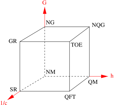
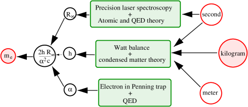

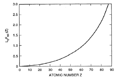
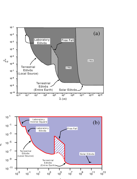
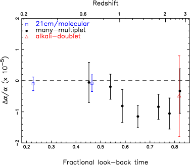
REFERENCES
- [1] Accetta, F.S., L.M. Krauss, and P. Romanelli, 1990, Phys. Lett. B 248, 146.
- [2] Agrawal, V., S.M. Barr, J. F. Donoghue, and D. Seckel, 1998a, Phys. Rev. D 57, 5480.
- [3] Agrawal, V., S.M. Barr, J. F. Donoghue, and D. Seckel, 1998b, Phys. Rev. Lett. 80, 1822.
- [4] Albrecht, A., and J. Magueijo, 1999, Phys. Rev. D 59, 043516.
- [5] Alexander, S.H.S., 2000, JHEP 0011, 017.
- [6] Anderson, J.D., J.K. Campbell, R.F. Jurgens, E.L. Lau, X.X. Newhall, M.A. Slade III, and E.M. Standish Jr., 1991, in Proceedings of the Marcel Grossmann meeting on general relativity, Kyoto, june 1991, edited by H. Sato and T. Nakamura (World Scientific, Singapore 1992), 353.
- [7] Armendáriz-Picón, C., 2002, preprint astro-ph/0205187.
- [8] Atkinson, A., 1968, Phys. Rev. 170, 1193.
- [9] Avelino, P.P., S. Esposito, G. Mangano, C.J. Martins, A. Melchiorri, G. Miele, O. Pisanti, G. Rocha, and T.P. Viana, 2001, Phys. Rev. D 64, 103505.
- [10] Avelino, P.P., C.J.A. Martins, and G. Rocha, 2000, Phys. Lett. B 483, 210.
- [11] Avelino, P.P., C.J. Martins, G. Rocha, and P. Viana , 2000, Phys. Rev. D 62, 123508.
- [12] Baessler, S., B.R. Heckel, E.G. Adelberger, J.H. Gundlach, U. Schmidt, and H.E. Swanson, 1999, Phys. Rev. Lett. 83, 3585.
- [13] Bahcall, J.N., and E.E. Salpeter, 1965, Astrophys. J. 142, 1677.
- [14] Bahcall, J.N., and M. Schmidt, 1967, Phys. Rev. Lett. 19, 1294.
- [15] Bahcall, J.N., W.L. Sargent, and M. Schmidt, 1967, Astrophys. J. 149, L11.
- [16] Banerjee, N., and D. Pavon, Class. Quant. 18, 593.
- [17] Banks, T., and M. Dine, 2001, JHEP 0110, 012.
- [18] Banks, T., M. Dine, and M.R. Douglas, 2002, Phys. Rev. Lett. 88, 131301.
- [19] Barrow, J.D., 1978, Month. Not. R. Astron. Soc. 184, 677.
- [20] Barrow, J.D., 1987, Phys. Rev. D 35, 1805.
- [21] Barrow, J.D., 1999, Phys. Rev. D 59, 043515.
- [22] Barrow, J.D., and C. O’Toole, 2001, Month. Not. R. Astron. Soc. 322, 585.
- [23] Barrow, J.D., and J. Magueijo, 1998, Phys. Lett. B 443, 104.
- [24] Barrow, J.D., and J. Magueijo, 1999a, Class. Quant. Grav. 16, 1435.
- [25] Barrow, J.D., and J. Magueijo, 1999b, Phys. Lett. B 447, 246.
- [26] Barrow, J.D., and J. Magueijo, 2001, Astrophys. J. Lett. (in press).
- [27] Barrow, J.D., J. Magueijo, and H.B. Sandvik, 2002a, preprint astro-ph/0202129.
- [28] Barrow, J.D., J. Magueijo, and H.B. Sandvik, 2002b, preprint astro-ph/0204357..
- [29] Barrow, J.D., H.B. Sandvik, and J. Magueijo, 2002c, Phys. Rev. D 65, 06350.
- [30] Battye, R.A., R. Crittenden, and J. Weller, 2001, Phys. Rev. D 63, 0453505.
- [31] Baum, W.A., and R. Florentin-Nielsen, 1976, Astrophys. J. 209, 319.
- [32] Bekenstein, J.D., 1979, Comments Astrophys. 8, 89.
- [33] Bekenstein, J.D., 1982, Phys. Rev. D 25, 1527.
- [34] Bekenstein, J.D., 1993, Phys. Rev. D 48, 3641.
- [35] Benabed, K., and F. Bernardeau, 2001, Phys. Rev. D 64, 083501.
- [36] Bergström, L., S. Iguri, and H. Rubinstein, 1999, Phys. Rev. D 60, 045005.
- [37] Bethe, H.A., and E.E. Salpeter, 1977, Quantum mechanics of one- and two-electron atoms, Plenum, New York.
- [38] Binétruy, P., 1999, Phys. Rev. D 60, 063502.
- [39] Binétruy, P., 2000, Int. J. Theor. Phys. 39, 1859.
- [40] Birge, R.T., 1929, Rev. Mod. Phys. 1, 1.
- [41] Blake, G.M., 1977a, Month. Not. R. Astron. Soc. 181, 47p.
- [42] Blake, G.M., 1977b, Month. Not. R. Astron. Soc. 181, 41p.
- [43] Bluhm, R., V.A. Kostelecký, C.D. Lane, and N. Russel, 2002, Phys. Rev. Lett. 88, 090801.
- [44] Brans, C., and R.H. Dicke, 1961, Phys. Rev. 124, 925.
- [45] Brax, P., and Davis, A.C., 2001, JHEP 0105, 007
- [46] Braxmaier, C., O. Pradl, H. Müller, A. Peters, J. Mlynek, V. Loriette, and S. Schiller, 2001, Phys. Rev. D 64, 042001.
- [47] Breakiron, L., 1993, in Proc. of the 25th Annual Precise Time Interval Applications and Planning Meeting (NASA Conf. Publ. No. 3267), 401.
- [48] Breit, G., 1930, Phys. Rev. 35, 1477.
- [49] Broulik, B., and J.S. Trefil, 1971, Nature (London) 232, 246.
- [50] Cahn, R.N., 1996, Rev. Mod. Phys. 68, 951.
- [51] Calmet, X., and H. Fritzsch, 2001, preprint hep-ph/0112110.
- [52] Calmet, X., and H. Fritzsch, 2001, preprint hep-ph/0204258.
- [53] Campbell, B.A., and K.A. Olive, 1995, Phys. Lett. B 345, 429-434.
- [54] Canuto, V.M., and I. Goldman, 1982, Nature (London) 296, 709.
- [55] Carilli, C.L., K.M. Menten, J.T.Stocke, E. Perlman, R. Vermeulen, F. Briggs, A.G. de Bruyn, J. Conway, and C.P. Moore, 2000, Phys. Rev. Lett. 85, 5511.
- [56] Carr, B.J., and M.J. Rees, 1979, Nature (London) 278, 605.
- [57] Carroll, S.M., 1998, Phys. Rev. Lett. 81, 3067.
- [58] Carroll, S.M., 2001, Living Rev. Rel. 4, 1.
- [59] Carroll, S.M., and M. Kaplinghat, 2001, preprint astro-ph/0108002.
- [60] Carter, B., 1974, in Confrontation of cosmological theories with observational data, IAU Symposia 63, edited by M. Longair (Reidel, Dordrecht) 291.
- [61] Carter, B., 1976, in Atomic physics and fundamental constants 5, edited by J.H. Sanders and A.H. Wapstra, (Plenum press, New York) 650.
- [62] Carter, B., 1983 Phil. Trans. R. Soc. London A 310, 347.
- [63] Carter, B., J.-P. Uzan, R. Battye, and A. Mennim, 2001, Class. Quant. Grav 18, 4871.
- [64] Casas, J.A., J. Garcia-Bellido, and N. Quiros, 1992a, Mod. Phys. Lett. A 7, 447.
- [65] Casas, J.A., J. Garcia-Bellido, and N. Quiros, 1992b, Phys. Lett. B 278, 94.
- [66] Chacko, Z., C. Grojean, and M. Perelstein, 2002, preprint hep-ph/0204142.
- [67] Chamoun, N., S.J. Landau, and H. Vucetich, 2000, preprint astro-ph/0009204.
- [68] Chamoun, N., S.J. Landau, and H. Vucetich, 2001, Phys. Lett. B 504, 1.
- [69] Chandler, J.F., R.D. Reasenberg, I.I. Shapiro, 1993, Bull. Am. Astron. Soc. 25, 1233.
- [70] Chandrasekhar, S., 1937, Nature (London) 139, 757.
- [71] Chen, X., and M. Kamionkowski, 1999, Phys. Rev. D 60, 104036.
- [72] Chiba, T., 2001, preprint gr-qc/0110118.
- [73] Chiba, T., and Khori, 2001, preprint hep-ph/0111086.
- [74] Chodos, A., and S. Detweiler, 1980, Phys. Rev. D 21, 2167.
- [75] Choi, K., 2000, phys. Rev. Lett. 85, 4434.
- [76] Chupp, T.E., R.J. Hoare, R.A. Loveman, E.R. Oteiza, J.M. Richardson, M.E. Wagshul, and A.K. Thompson, 1989, Phys. Rev. Lett. 63, 1541.
- [77] Clayton, M.A., and J.W. Moffat, 1998, Phys. Lett. B 460, 263.
- [78] Clayton, M.A., and J.W. Moffat, 2000, Phys. Lett. B 477, 275.
- [79] Clayton, M.A., and J.W. Moffat, 2001, Phys. Lett. B 506, 177.
- [80] Cohen-Tannoudji, C., B. Diu, and F. Laloë, 1986, Mécanique Quantique, Ed. Hermann.
- [81] Cohen-Tannoudji, G., 1995, Les constantes universelles, Coll. Questions de sciences (Hachette, Paris)
- [82] Coley, A.A., 1990, Astron. Astrophys. 233, 305.
- [83] Counselman, C.C., and I.I. Shapiro, 1968, Science 162, 352.
- [84] Cowie, L.L., and A. Songaila, 1995, Astrophys. J. 453, 596.
- [85] Creer, K.M., 1965, Nature (London) 206, 539.
- [86] Cremmer, E., and J. Scherk, 1977, Nuc. Phys. B 118, 61.
- [87] Damour, T., 1996, Class. Quant. Grav. 13, A33.
- [88] Damour, T., 2001, in the Proceedings of the workshop Missions spatiales en physique fondamentale (Chatillon, 18-19 Jan. 2001), Comptes Rendus de l’Academie des Sciences (Paris), edited by C. Borde and P. Touboul.
- [89] Damour, T., and F.J. Dyson, 1996, Nuc. Phys. B 480, 37.
- [90] Damour, T., and G. Esposito-Farèse, 1992, Class. Quant. Grav. 9, 2093.
- [91] Damour, T., and C. Gundlach, 1991, Phys. Rev. D 43, 3873.
- [92] Damour, T., and B. Pichon, 1999, Phys. Rev. D 59, 123502.
- [93] Damour, T., and A.M. Polyakov, 1994a, Nuc. Phys. B 423, 532.
- [94] Damour, T., and A.M. Polyakov, 1994b, Gen. Rel. Grav. 26, 1171.
- [95] Damour, T., and J.H. Taylor, 1991, Astrophys. J. 366, 501.
- [96] Damour, T., G.W. Gibbons, and C. Gundlach, 1990, Phys. Rev. Lett. 64, 123.
- [97] Damour, T., G.W. Gibbons, and J.H. Taylor, 1988, Phys. Rev. Lett. 61, 1151.
- [98] Damour, T., F. Piazza, and G. Veneziano, 2002a, preprint gr-qc/0204094.
- [99] Damour, T., F. Piazza, and G. Veneziano, 2002b, preprint hep-th/0205111.
- [100] Davies, P.C.W., 1972, J. Phys. A 5, 1296.
- [101] Dearborn, D.S., and D.N. Schramm, 1974, Nature (London) 247, 441.
- [102] Del’Innocenti, S., G. Fiorentini, G.G. Raffelt, B. Ricci, and A. Weiss, 1996, Astron. Astrophys. 312, 345.
- [103] de Bernardis, P., 2000, Nature (London) 404, 955.
- [104] Demarque, P., L.M. Krauss, D.B. Guenther, and D. Nydam, 1994, Astrophys. J. 437, 870.
- [105] Demidov N.A., et al., 1992, in Proceedings of the 6th European frequency and time forum, Noordwijk, NL, 1992, (European Space Agency, Noordwjik) 409.
- [106] Dent, T., and M. Fairbairn, 2001, preprint hep-ph/0112279.
- [107] de Witt, B.S., 1964, Phys. Rev. Lett. 13, 114.
- [108] Dicke, R.H., 1957, Rev. Mod. Phys. 29, 355.
- [109] Dicke, R.H., 1959, Nature (London) 183, 170.
- [110] Dicke, R.H., 1961, Nature (London) 192, 440.
- [111] Dicke, R.H., 1962a, Rev. Mod. Phys. 34 110.
- [112] Dicke, R.H., 1962b, Phys. Rev. 125, 2163.
- [113] Dicke, R.H., 1962c, Science 138, 653.
- [114] Dicke, R.H., 1964, in Relativity, Groups and Topology, Lectures delivered at Les Houches 1963, edited by C. DeWitt and B. DeWitt, (Gordon and Breach, New York).
- [115] Dicke, R.H., 1969, Gravitation and the universe, American Philosophical Society (Philadelphia).
- [116] Dicke, R.H., and P.J.E. Peebles, 1965, Space Sci. Rev. 4, 419.
- [117] Dickey, J.O., et al., 1994, Science 265, 482.
- [118] Dicus, D.A., E.W. Kolb, A.M. Gleeson, E.C.G. Sudarshan, V.L. Teplitz, and M.S. Turner, 1982, Phys. Rev. D 26, 2694.
- [119] Dirac, P.A.M., 1937, Nature (London) 139, 323.
- [120] Dirac, P.A.M., 1938, Proc. Roy. Soc. London A 165, 198.
- [121] Dirac, P.A.M., 1974, Proc. Roy. Soc. London A 338, 439.
- [122] Dirac, P.A.M., 1979, Proc. Roy. Soc. London A 365, 19.
- [123] Dixit, V.V., and M. Sher, 1988, Phys. Rev. D 37, 1097.
- [124] Drinkwater, M.J., J.K. Webb, J.D. Barrow, and V.V. Flambaum, 1998, Month. Not. R. Astron. Soc. 295, 457.
- [125] Dudas, E., 2000, Class. Quant. Grav. 17, R41.
- [126] Duff, M.J., L.B. Okun, and G. Veneziano, 2002, JHEP 0203, 37.
- [127] Durrer, R, 2002, J. Phys. Stud., in press.
- [128] Dvali, G., and M. Zaldarriaga, 2002, Phys. Rev. Lett. 88, 091303.
- [129] Dyson, F.J., 1967, Phys. Rev. Lett. 19, 1291.
- [130] Dyson, F.J., 1971, Sc. Am. 225, 51.
- [131] Dyson, F.J., 1972, in Aspects of Quantum Theory, edited by A. Salam and E.P. Wigner (Cambridge University Press, Cambridge) 213-236.
- [132] Dyson, F.J., 1978, in Current Trends in the Theory of Fields, Proceedings of the Symposium in honor of P.A.M. Dirac, Tallahassee, Florida, 1978, AIP Conf. Proc. No. 48, edited by J.E. Lannutti and P.K. Williams (American Institute of Physics, New York) 163.
- [133] Dzuba, V.A., V.V. Flambaum, and O.D. Sushkov, 1983, J. Phys. B 16, 715.
- [134] Dzuba, V.A., V.V. Flambaum, and M.G. Kozlov, 1996, Phys. Rev. A 54, 3948.
- [135] Dzuba, V.A., V.V. Flambaum, and J.K. Webb, 1999a, Phys. Rev. A 59 230.
- [136] Dzuba, V.A., V.V. Flambaum, and J.K. Webb, 1999b, Phys. Rev. Lett.82, 888..
- [137] Dzuba, V.A., V. V. Flambaum, M. T. Murphy, and J. K. Webb, 2001, Phys. Rev. A 63, 042509.
- [138] Eardley, D.M., 1975, Astrophys. J. 196, L59.
- [139] Egyed, L., 1961, Nature (London) 190, 1097.
- [140] Eötvös, R.V., D. Pekár, and E. Fekete, 1922, Ann. Phys. (Leipzig) 68, 11.
- [141] Esposito-Farèse, G., and D. Polarski, 2001, Phys. Rev. D 63, 063504.
- [142] Ezer, D., and A.G.W. Cameron, 1966, Can. J. Phys. 4, 593.
- [143] Fierz, M., 1956, Helv. Phys. Acta 29, 128.
- [144] Fischbach, E., and C. Talmadge, 1996, Proc. of the XXXIth Rencontres de Moriond, Les Arcs (France) 20-27 january 1996.
- [145] Flambaum, V.V., and E.V. Shuryak, 2001, preprint hep-ph/0201303.
- [146] Flowers, J.L., and B.W. Petley, 2001, Rept. Prog. Phys. 64, 1191.
- [147] Foltz, C.B., F.H. Chaffee, and J.H. Black, 1988, Astrophys. J. 324, 1988.
- [148] Forgács, P., and Z. Horváth, 1979, Gen. Rel. Grav. 10, 931.
- [149] Fowler, W.A., G.R. Caughlan, and B.A. Zimmerman, 1975, Annu. Rev. Astron. Astrophys. 13, 69.
- [150] Freund, P.G.O., 1982, Nuc. Phys. B 209, 146.
- [151] Fujii, Y., A. Iwamoto, T. Fukahori, T. Ohnuki, M. Nakagawa, H. Hidaka, Y. Oura, and P. Möller, 2000, Nuc. Phys. B 573 377.
- [152] Fujii, Y., 2002, preprint astro-ph/0204069.
- [153] Gamow, G., 1967a, Phys. Rev. Lett. 19, 759.
- [154] Gamow, G., 1967b, Phys. Rev. Lett. 19, 913.
- [155] Gamow, G., 1967c, Proc. Natl. Acad. Sci. U.S. 57, 187.
- [156] Gasperini, M., F. Piazza, and G. Veneziano, 2002, Phys. Rev. D 65, 023508.
- [157] Gasser, J., and H. Leutwyler, 1982, Phys. Rep. 87, 77
- [158] Gaztañaga, E., E. Garcia-Berro, J. Isern, E. Bravo, and I. Dominguez, 2002, Phys. Rev. D 65, 023506.
- [159] Georgi, H. Quinn H., and S. Weinberg, 1974, Phys. Rev. Lett. 33, 451.
- [160] Gold, R., 1968, Phys. Rev. Lett. 20, 219.
- [161] Godone, A., C. Novero, P. Tavella, and K. Rahimullah, 1993, Phys. Rev. Lett. 15, 2364.
- [162] Goldman, I., 1990, Month. Not. R. astr. Soc. 244, 184.
- [163] Guenther, L.M. Krauss, and P. Demarque, 1998, Astrophys. J. 498, 871.
- [164] Guenther, D.B., K. Sills, P. Demarque, and L.M. Krauss, 1995, Astrophys. J. 445, 148.
- [165] Gundlach, J.H., and S.M. Merkowitz, 2000, Phys. Rev. Lett. 85, 2869.
- [166] Hannestad, S., 1999, Phys. Rev. D 60, 023515.
- [167] Harko, T., and M.K. Mak, 1999, Class. Quant. Grav. 16, 2741.
- [168] Haugan, M.P., and C.M. Will, 1976, Phys. Rev. Lett. 37, 1.
- [169] Haugan, M.P.,1979, Ann. Phys. (NY) 118, 156.
- [170] Heintzmann, H., and H. Hillebrandt, 1975, Phys. Lett. A 54, 349.
- [171] Hellings, R.W., P.J. Adams, J.D. Anderson, M.S. Keesey, E.L. Lau, E.M. Standish, V.M. Canuto, and I. Goldman, 1983, Phys. Rev. Lett. 51, 1609.
- [172] Hill, H.A., and Y.-M. Gu, 1990, Sci. China A 37, 854.
- [173] Hoffmann, D.C., F.O. Lawrence, J.L. Mewherter, and F.M. Rourke, 1971, Nature (London) 234, 132.
- [174] Hogan, C.J., 2000, Rev. Mod. Phys. 72, 1149.
- [175] Hořava, P., and E. Witten, 1996, Nuc. Phys. B 460, 506.
- [176] Horváth, J.E., and H. Vucetich, 1988, Phys. Rev. D 37, 931.
- [177] Hoyle, F., 1972, Q. Jl. R. astr. Soc. 13, 328.
- [178] Hu, W., and S. Dodelson, 2002, Ann. Rev. Astron. Astrophys. (2002) in press.
- [179] Huey, G., S. Alexander, and L. Pogosian, 2001, preprint astro-ph/0110562.
- [180] Ichikawa, K., and M. Kawasaki, 2002, preprint hep-ph/0203006.
- [181] Irvine, J.M., 1983a, Phil. Trans. R. Soc. London a 310, 239.
- [182] Irvine, J.M., 1983b, Contemp. Phys. 24, 427.
- [183] Isham, C.J., A. Salam, and J. Strathdee, 1971, Phys. Rev. D 3, 1805.
- [184] Itzykson, C., and J-B. Zuber, 1980, Quantum field theory, MacGraw-Hill, New York.
- [185] Ivanchik, A.V., A.Y. Potekhin, and D.A. Varshalovich, 1999, Astron. Astrophys. 343, 439.
- [186] Ivanchik, A.V., E. Rodriguez, P. Petitjean, and D. Varshalovich, 2001, preprint astro-ph/0112323.
- [187] Jordan, P., 1937, Naturwiss. 25, 513.
- [188] Jordan, P., 1939, Z. Physik 113, 660.
- [189] Jordan, P., 1955, Schwerkraft und Weltall, (Vieweg, Braunschweig).
- [190] Kaluza, T., 1921, Sitzungsber. Preuss. Akad. Wiss. Phys. Math. Kl. LIV, 966.
- [191] Kaplinghat, M., R.J. Scherrer, and M.S. Turner, 1999, Phys. Rev. D 60, 023516.
- [192] Kaspi, V.M., J.H. Taylor, and M.F. Riba, 1994, Astrophys. J. 428, 713.
- [193] Kehagias, A., and E. Kiritsis, 1999, JHEP 9911, 022.
- [194] Khare, P., 1986, Phys. Rev. D 34, 1936.
- [195] Kim. J.B., and H.K. Lee, 1995, Astrophys. J. 448, 510.
- [196] Kim. J.B., J.H. Kim, and H.K. Lee, 1998, Phys. Rev. D 58, 027301.
- [197] Kiritsis, E., 1999, JHEP 9910, 010.
- [198] Karshenboim, S.G., 2000, Can. J. Phys. 78, 639.
- [199] Karshenboim, S.G., 2001, in Laser Physics at the Limits, edited by H. Figger, D. Meschede and C. Zimmermann, (Springer-Verlag, Berlin, Heidelberg), 165.
- [200] Klein, O., 1926, Z. Phys. 37, 875.
- [201] Kolb, E.W., M.J. Perry, and T.P. Walker, 1986, Phys. Rev. D 33, 869-871.
- [202] Kothari, D.S., 1938, Nature (London) 142, 354.
- [203] Kujat, J., and R.J. Scherrer, 2000, Phys. Rev. D 62, 023510.
- [204] Lamoreaux, S.K., J.P. Jacobs, B.R. Heckel, F.J. Raab, and E.N. Fortson, 1986, Phys. Rev. Lett. 57, 3125.
- [205] Landau, L.D., 1955, in Niels Bohr and the development of physics, edited by W. Pauli (Pergamon press, London).
- [206] Landau, S., and H. Vucetich, 2000, preprint astro-ph/0007108.
- [207] Landau, S., and H. Vucetich, 2002, Astrophys. J. 570, 463.
- [208] Landau, S., D.D. Harai, and M. Zaldarriaga, 2001, Phys. Rev. D 63, 083505.
- [209] Langacker, P., G. Segrè, and M.J. Strassler, 2002, Phys. Lett. B 528, 121
- [210] Lanzetta, K.M., et al., 1995, in proc. of the XVIIyh Texas symposiumon relativistic astrophysics, edited by W. Voges.
- [211] Levshakov, S.A., 1992, ESO conf. Proc. 40, 139.
- [212] Levy-Leblond, J.M., 1979, in Problems in the foundations of physics, LXXII corso, (societa Italiana di Fisica Bologna), 237-263.
- [213] Li, L.-X., and R. Gott III, 1998, Phys. Rev. D 58, 103513.
- [214] Lichnérowicz, A., 1955, Théories relativistes de la gravitation et de l’électromagnétisme, Ed. Masson and Cie, Paris, France.
- [215] Lindner, M., D.A. Leich, R.J. Borg, G.P. Russ, J.M. Bazan, D.S. Simons, and A.R. Date, 1986, Nature (London) 320, 246.
- [216] Livio, M., and M. Stiavelli, 1998, Astrophys. J. 507, L13.
- [217] Livio, M., D. Hollowell, A. Weiss, Nature (London) 340, 281.
- [218] Lubo, M., M. Lemoine, J. Martin, and J.-P. Uzan, 2002, Phys. Rev. D 65, 023510.
- [219] Lynden-Bell, D., 1982, Observatories 102, 86.
- [220] Ma, C.-P., and E. Bertschinger, 1995, Astrophys. J. 455, 7.
- [221] Magueijo, J., 2000, Phys. Rev. D 62, 103521.
- [222] Magueijo, J., 2001, Phys. Rev. D 63, 043502.
- [223] Magueijo, J., H.B. Sandvik, and T.W.B. Kibble, 2001, Phys. Rev. D 64, 023521.
- [224] Magueijo, J., J.D. Barrow, and H.B. Sandvik, 2002, preprint astro-ph/0202374.
- [225] Malaney, R.A., and G.J. Mathews, 1993, Phys. Rep. 229, 145.
- [226] Mansfield, 1976, Nature (London) 261, 560.
- [227] Marciano, W.J., 1984, Phys. Rev. Lett. 52, 489.
- [228] Martins, C.J.A.P., 2002, preprint atro-ph/0205504.
- [229] Martins, C.J.A.P., A. Melchiorri, R. Trotta, R. Bean, G. Rocha, P.P. Avelino, and P.T.P. Viana, 2002, preprint atro-ph/0203149.
- [230] Maurette, M. 1976, Ann. Rev. Nuc. Sci. 26, 319.
- [231] Mellier, Y., 1999, Ann. Rev. Astron. Astrophys. 37, 127.
- [232] McElhinny, M.W., S.R. Taylor, and D.J. Stevenson, 1978, Nature (London) 271, 316.
- [233] McWeeny, R., 1973, Nature (London) 243, 196.
- [234] Milne, E.A., 1935, Proc. Roc. Soc. London A 158, 324.
- [235] Minkowski, R., and O.C. Wilson, 1956, Astrophys. J. 123, 373.
- [236] Moffat, J., 1993a, Int. J. Phys. D 2, 351.
- [237] Moffat, J., 1993b, Found. Phys. 23, 411.
- [238] Moffat, J., 2001, preprint astro-ph/0109350.
- [239] Moffat, J., 2002, preprint gr-qc/0202012.
- [240] Mohr, J.-P., and B.N. Taylor, 2001, Phys. Today 54(3), 29.
- [241] Morrison, L.V., 1973, Nature (London) 241, 519.
- [242] Muller, P.M., 1978, in On the measurement of Cosmological Variations of the gravitaional constant, edited by L. Halphern, University of Florida, p. 93.
- [243] Müller, J., and K. Nordtvedt, 1998, Phys. Rev. D 58, 062001.
- [244] Müller, J., M. Schneider, K. Nordtvedt, and D. Vokrouhlicky, 1999, in Proceedings of the 8th Marcel Grossman Meeting on General Relativity, Jerusalem, 1997 (World Scientific, Singapore).
- [245] Müller, J., M. Schneider, M. Soffel, and H. Ruder, 1991, Astrophys. J. 382, L101.
- [246] Murphy, C.T., and R.H. Dicke, 1964, Proc. Am. Phil. Soc. 108, 224.
- [247] Murphy, M.T., J.K. Webb, V.V. Flambaum, C.W. Churchill, J.X. Prochaska, 2001b, Month. Not. R. Astron. Soc. 327, 1223.
- [248] Murphy, M.T., J.K. Webb, V.V. Flambaum, M.J. Drinkwater, F. Combes, and T. Wiklind, 2001, Month. Not. R. Astron. Soc. 327, 1244.
- [249] Murphy, M.T., J.K. Webb, V.V. Flambaum, V.A. Dzuba, C.W. Churchill, J.X. Prochaska, J.D. Barrow, and A.M. Wolfe, 2001, Month. Not. R. Astron. Soc. 327, 1208.
- [250] Murphy, M.T., J.K. Webb, V.V. Flambaum, J.X. Prochaska, and A.M. Wolfe, 2001, Month. Not. R. Astron. Soc. 327, 1237.
- [251] Murray, C., and S. Dermott, 2000, Solar System Dynamics, Cambridge University Press.
- [252] Naudet, R., 1974, Bull. Inf. Sci. Tech. (Paris) 193, 1.
- [253] Naudet, R., 2000, Oklo, des réacteurs nucléaires fossiles: étude physique, Editions du CEA (France).
- [254] Newton, R.R., 1970, Ancient Astronomical observations and Acceleration of the Earth and Moom, John Hopkins Press (Baltimore).
- [255] Newton, R.R., 1974, Month. Not. R. astr. Soc. 169, 331.
- [256] Noerdlinger, P.D., 1973, Phys. Rev. Lett. 30, 761.
- [257] Nollet, K.M., and R.E. Lopez, 2002, preprint astro-ph/0204325.
- [258] Nordtvedt, K., 1988, Phys. Rev. D 37, 1070.
- [259] Nordtvedt, K., 1990, Phys. Rev. Lett. 65, 953.
- [260] Nordtvedt, K., 2001, Class. Quant. Grav. 18, L133.
- [261] Novikov, I.D., and Ya. B. Zel’dovich, 1982, The structure and evolution of the universe, part V, University of Chicago Press.
- [262] Oberhummer, H., A. Csótó, and H. Schlattl, 2000, Science 289, 88.
- [263] Okun, L.B., 1991, Usp. Fiz. Nauk. 161, 177 [Sov. Phys. Usp. 34, 818].
- [264] Olive, K., and M. Pospelov, 2001, preprint hep-ph/0110377.
- [265] Olive, K., M. Pospelov, Y.-Z. Qian, A. Coc, M. Cassé, and E. Vangioni-Flam, 2002, preprint hep-ph/0205269.
- [266] Overduin, J.M., and P.S. Wesson, 1997, Phys. Rep. 283, 303.
- [267] Pagel, B.E.J., 1977, Month. Not. R. Astron. Soc. 179, 81.
- [268] Pagel, B.E.J., 1983, Phil. Trans. R. Soc. Lond. A 310, 245.
- [269] Passarino, G., 2001, preprint hep-ph/0108524.
- [270] Peebles, P.J.E., 1968, Astrophys. J. 153, 1.
- [271] Peebles, P.J., and R.H. Dicke, 1962, Phys. Rev. 128 2006.
- [272] Peres, A., 1967, Phys. Rev. Lett. 19, 1293.
- [273] Perlmutter, S., et al., 1998, Nature (London) 391, 51.
- [274] Petley, B.W., 1983, Nature (London) 303, 373.
- [275] Petley, B.W., 1985, The fundamental physical constants and the frontiere of measurement, (Adam Hilger, Bristol and Philadelphia).
- [276] Petrov, Y.V., 1977, Sov. Phys. Usp. 20, 937.
- [277] Pochet, T., J.M. Pearson, G. Beaudet, and H. Reeves, 1991, Astron. Astrophys, 243, 1.
- [278] Pochoda, P., and M. Schwarzschild, 1963, Astrophys. J. 139, 587.
- [279] Polchinsky, J., 1997, Superstring Theory, Cambridge University Press, UK.
- [280] Potekhin, A.Y., and D.A. Varshalovich, 1994, Astron. Astrophys. Suppl. Ser. 104, 89.
- [281] Potekhin, A.Y., A.V. Ivanchik, D.A. Varshalovich, K.M. Lanzetta, J.A. Baldwin, G.M. Williger, and R.F. Carswell, 1998, Astrophys. J. 505, 523.
- [282] Prestage, J.D., R.L. Tjoelker, and L. Maleki, Phys. Rev. Lett. 74, 3511.
- [283] Prochoska, J.X., and A.M. Wolfe, 1996, Astrophys. J. 470, 403.
- [284] Prochoska, J.X., and A.M. Wolfe, 1997, Astrophys. J. 474, 140.
- [285] Prochoska, J.X., and A.M. Wolfe, 2000, Astrophys. J. 533, L5.
- [286] Rañada, A.F., 2002, preprint astro-ph/0202224.
- [287] Reasenberg, R.D., and I.I. Shapiro, 1976, in Atomic masses and fundamental constants, Vol. 5, edited by J.H. Sanders and A.H. Wapstra (Plenum, New York), 643.
- [288] Reasenberg, R.D., and I.I. Shapiro, 1978, in On the measurements of cosmological variations of the gravitational constant, edited by L. Halperin (University of Florida, Gainesville), 71.
- [289] Reasenberg, R.D., 1983, Phil. Trans. R. Soc. Lond. A 310, 227.
- [290] Reeves, H., 1994, Rev. Mod. Phys. 66, 193.
- [291] Riazuelo, A., and J.-P. Uzan, 2000, Phys. Rev. D 62, 083506.
- [292] Riazuelo, A., and J.-P. Uzan, 2002, Phys. Rev. D 65 (to appear); preprint astro-ph/0107386.
- [293] Ricci, B., and F.L. Villante, 2002, preprint astro-ph/0204482.
- [294] Riess, A.G., et al., 1998, Astron. J. 116, 1009.
- [295] Roeder, R.C., 1967, Astrophys. J. 149, 131.
- [296] Rothman, T., and R. Matzner, 1982, Astrophys. J. 257, 450.
- [297] Rozental, I.L., 1980, Usp. Fiz. Nauk. 131, 239; [Sov. Phys. Usp. 23 (1980) 296].
- [298] Rozental, I.L., 1988, Big Bang, Big Bounce (Springer-Verlag, Berlin).
- [299] Runcorn, S.K., 1964, Nature (London) 204, 823.
- [300] Sandvik, H.B., J.D. Barrow, and J. Magueijo, 2002, Phys. Rev. Lett. 88, 031302.
- [301] Savedoff, M.P., 1956, Nature (London) 176, 688.
- [302] Scherrer, R.J., and D.N. Spergel, 1993, Phys. Rev. D 47, 4774.
- [303] Scrutton, C.T., 1965, Paleontology 7, 552.
- [304] Serna, A., and R. Domínguez-Tenreiro, 1992, Astophys. J. 389, 1.
- [305] Serna, A., R. Domínguez-Tenreiro, and G. Yepes, 1992, Astophys. J. 391, 433.
- [306] Shapiro, I.I., 1964, Phys. Rev. Lett. 13, 789.
- [307] Shapiro, I.I., 1990, in General Relativity and Gravitation, edited by N. Ashby, D.F. Bartlett, and W. Wyss, Cambridge University Press.
- [308] Shapiro, I.I., W.B. Smith, and M.B. Ash, 1971, Phys. Rev. Lett. 26, 27.
- [309] Shlyakhter, A.I., 1976, Nature (London) 264, 340.
- [310] Silk, J., 1968, Astrophys. J. 151, 459.
- [311] Sisterna, P., and H. Vucetich, 1990, Phys. Rev. D 41 1034.
- [312] Sisterna, P., and H. Vucetich, 1991, Phys. Rev. D 44 3096.
- [313] Solheim, J.-E., T.G. Barnes III, and H.J. Smith, 1976, Astrophys. J. 209, 330.
- [314] Sortais, Y., et al., 2001, Physica Scripta T95, 50.
- [315] Stanyukovich, K.P., 1962, Dokl. Akad. Nauk. 147, 1348 [Sov. Phys. Dokl. 7, 1150 (1962)].
- [316] Steer, D., and M.P. Parry, 2002, preprint hep-th/0201121.
- [317] Steigmann, G., 1976, Nature (London) 261, 479.
- [318] Su, Y., B.R. Heckel, E.G. Adelberger, J.H. Gundlach, M. Harris, G.L. Smith, and H.E. Swanson, 1994, Phys. Rev. D 50, 3614.
- [319] Taylor, T.R., and G. Veneziano, 1988, Phys. Lett. B 213, 450.
- [320] Teller, E., 1948, Phys. Rev. 73, 801.
- [321] Thompson, R., 1975, Astron. Lett. 16, 3.
- [322] Thorsett, S.E., 1996, Phys. Rev. Lett. 77, 1432.
- [323] Torgerson, J.R., 2000, preprint physics/0012054.
- [324] Tubbs, A.D., and A.M. Wolfe, 1980, Astrophys. J. 236, L105.
- [325] Turneaure, J.P., and S.R. Stein, 1974, in Atomic masses and fundamental constants, Vol. 5, edited by J.H. Sanders and A.H. Wapstra (Plenum, New York) 636.
- [326] Uzan, J.-P., 1999, Phys. Rev. D 59, 123510.
- [327] Uzan, J.-P., 2002, Pour la Science (to appear, july).
- [328] Uzan, J.-P., and F. Bernardeau, 2001, Phys. Rev. D 64, 083004.
- [329] Van Diggelen, J., 1976, Nature (London) 262, 275.
- [330] Van Flandern, T.C., 1971, Astron. J. 76, 81.
- [331] Van Flandern, T.C., 1975, Month. Not. R. Astron. Soc. 170, 333.
- [332] Van Flandern, T.C., 1981, in Precision measurements and fundamental constants II, NBS circular No. 617 (U.S. GPO., Whashington DC) 625.
- [333] Vanier, J., and C. Audouin, 1989, The quantum physics of atomic frequency standards, Adam Hilger (Bristol and Philadelphia).
- [334] Varshalovich, D.A., and S.A. Levshakov, 1993, J. Exp. Theor. Phys. Lett, 58, 231.
- [335] Varshalovich, D.A., A.Y. Potekhin, 1994, Astron. Lett. 20, 771.
- [336] Varshalovich, D.A., A.Y. Potekhin, 1995, Space Sci. Rev. 74, 259.
- [337] Varshalovich, D.A. and A.Y. Potekhin, 1996, Astron. Lett. 22, 1.
- [338] Varshalovich, D.A., V.E. Panchuk, A.V. Ivanchik, 1996b, Astron. Lett. 22, 6.
- [339] Varshalovich, D.A., A.Y. Potekhin, A.V. Ivanchik, V.E. Panchuk, and K.M. Lanzetta, 1996a, Proceedings of the Second International Sakharov Memorial Conference (Moscow, 19-26 May, 1996).
- [340] Varshalovich, D.A., A.Y. Potekhin, and A.V. Ivanchik, 2000b, Comments At. Mol. Phys. (to appear), preprint physics/0004068.
- [341] Varshalovich, D.A., A.Y. Potekhin, and A.V. Ivanchik, 2000a, in X-ray and Inner-Shell Processes, AIP Conf. Proc. (AIP, Melville, 2000), edited by R.W. Dunford, D.S. Gemmel, E.P. Kanter, B. Kraessig, S.H. Southworth, and L. Young, 506, 503.
- [342] Vayanokis, C.E., 1988, Phys. Lett. B 213, 419.
- [343] Veneziano, G., 1986, Europhysics Lett. 2, 199.
- [344] Vila, S.C., 1976, Astrophys. J. 206, 213.
- [345] Vinti, J.P., 1974, Month. Not. R. Soc. 169, 417.
- [346] Volovik, G.E., 2002, preprint physics/0203075.
- [347] Webb, J.K., V.V. Flambaum, C.W. Churchill, M.J. Drinkwater, J.D. Barrow, 1999, Phys. Rev. Lett. 82, 884.
- [348] Webb, J.K., M.T. Murphy, V.V. Flambaum, V.A. Dzuba, J.D. Barrow, C.W. Churchill, J.X. Pochaska, and A.M. Wolfe, 2001, Phys. Rev. Lett. 87, 091301.
- [349] Weinberg, S., 1983a, Phil. Trans. R. Soc. London A 310, 249.
- [350] Weinberg, S., 1983b, Phys. Lett. B 125, 265.
- [351] Weinberg, S., 1989, Rev. Mod. Phys. 61, 1.
- [352] Wesson, P.S., 1973, Q. Jl. astr. Soc. 14, 9.
- [353] Wetterich, C., 2002, preprint hep-ph/0203266.
- [354] Wignall, J.W.G., 2000, Int. J. Mod. Phys. A 15, 875-892.
- [355] Wiklind, T., and F. Combes, 1997, Astron. Astrophys. 328, 48.
- [356] Wilkinson, D.H., 1958, Phil. Mag. 3, 582.
- [357] Will, C.M., 1993, Theory and experiment in gravitaional physics, (Cambridge University Press).
- [358] Will, C.M., 2001, Living Rev. Relativity 4, 4.
- [359] Williams, P.J., et al., 1976, Phys. Rev. Lett. 36, 551.
- [360] Williams, P.J., X.X. Newhall, and J.O. Dickey, 1996, Phys. Rev. D 53, 6730-6739.
- [361] Witten, E., 1981, Nuc. Phys. B 186, 412.
- [362] Witten, E., 1984, Phys. Lett. B 149, 351.
- [363] Wolfe, A.M., R.L. Brown and M.S. Roberts, 1976, Phys. Rev. Lett. 37, 179.
- [364] Wolfe, A.M., and M.M. Davis, 1979, Astron. J. 84, 699.
- [365] Wu, Y.S., and Z. Wang, 1986, Phys. Rev. Lett. 57, 1978.
- [366] Yahil, 1975, in The interaction between science and philosophy, edited by Y. Elkana, Humanities Press, 27.
- [367] Yang, J., D.N. Schramm, G. Steigmann, and R.T. Rood, 1979, Astrophys. J. 227, 697.
- [368] Youm, D., 2001, preprint hep-th/0108237.
| Comparison | constant |
|---|---|
| fine structure doublet | |
| hyperfine H vs optical | |
| hyperfine H vs fine-structure | |
| rotational vs vibrational modes of molecules | |
| rotational modes vs hyperfine H | |
| fine structure doublet vs hyperfine H |
| Reference | Constraint | Redshift | Time () | Method |
|---|---|---|---|---|
| (Savedoff, 1956) | 0.057 | Cygnus A (N II, Ne III) | ||
| (Wilkinson, 1958) | 3-4 | -decay | ||
| (Bahcall et al., 1967) | 1.95 | QSO (Si II, Si IV) | ||
| (Bahcall and Schmidt, 1967) | 0.2 | radio galaxies (O III) | ||
| (Dyson, 1967) | 3 | Re/Os | ||
| (Gold, 1968) | 2 | Fission | ||
| (Chitre and Pal, 1968) | 1 | Fission | ||
| (Dyson, 1972) | 2 | -decay | ||
| (Dyson, 1972) | 2 | Fission | ||
| (Dyson, 1972) | 1 | Re/Os | ||
| (Shlyakhter, 1976) | 1.8 | Oklo | ||
| (Wolfe et al., 1976) | 0.524 | QSO (Mg I) | ||
| (Irvine, 1983a) | 1.8 | Oklo | ||
| (Lindner et al., 1986) | 4.5 | Re/Os | ||
| (Kolb et al., 1986) | BBN | |||
| (Potekhin and Varshalovich, 1994) | 3.2 | QSO (C IV, Si IV,…) | ||
| (Varshalovich and Potekhin, 1994) | 3.2 | QSO (C IV, Si IV,…) | ||
| (Cowie and Songaila, 1995) | QSO | |||
| (Prestage et al., 1995) | 0 | 140 days | Atomic cloks | |
| (Damour and Dyson, 1996) | 1.8 | Oklo | ||
| (Varshalovich et al., 1996a) | QSO (Si IV) | |||
| (Bergström et al., 1999) | BBN | |||
| (Webb et al., 1999) | QSO (Mg II, Fe II) | |||
| (Webb et al., 1999) | QSO (Mg II, Fe II) | |||
| (Ivanchik et al., 1999) | QSO (Si IV) | |||
| (Fujii et al., 2000) | 1.8 | Oklo | ||
| (Varshalovich et al., 2000a) | QSO (Si IV) | |||
| (Avelino et al., 2001) | CMB | |||
| (Landau et al., 2001) | CMB | |||
| (Webb et al., 2001) | QSO (Fe II, Mg II) | |||
| (Webb et al., 2001) | QSO (Ni II, Cr II, Zn II) | |||
| (Webb et al., 2001) | QSO (Si IV) | |||
| (Murphy et al., 2001a) | QSO (Mg I, Mg II,…) | |||
| (Murphy et al., 2001a) | QSO (Mg I, Mg II,…) | |||
| (Murphy et al., 2001a) | QSO (Mg I, Mg II,…) | |||
| (Murphy et al., 2001d) | QSO (Si IV) | |||
| (Sortais et al., 2001) | 24 months | Atomic clock | ||
| (Nollet and Lopez, 2002) | BBN | |||
| (Ichikawa and Kawasaki, 2002) | BBN | |||
| (Olive et al., 2002) | 1.8 | Oklo | ||
| (Olive et al., 2002) | 4.6 | Re/Os | ||
| (Olive et al., 2002) | -decay |
| Reference | Experiment | Constant | Duration | Limit () |
|---|---|---|---|---|
| (Turneature and Stein, 1974) | hfs of Cs vs SCO | 12 days | ||
| (Godone et al., 1983) | hfs of Cs vs fs of Mg | 1 year | ||
| (Demidov, 1992) | hfs of Cs vs hfs of H | 1 year | ||
| (Breakiron, 1993) | hfs of Cs vs hfs of H | |||
| (Prestage et al., 1995) | hfs of HG+ vs hfs of H | 140 days | ||
| (Sortais et al., 2001) | hfs of Cs vs hfs of Rb | 24 months |
| Reference | Constraint (yr-1) | Method |
|---|---|---|
| (Teller, 1948) | Earth temperature | |
| (Shapiro at al., 1971) | Planetary ranging | |
| (Morison, 1973) | Lunar occultations | |
| (Dearborn and Schramm, 1974) | Clusters of galaxies | |
| (van Flandern, 1975) | Lunar occultations | |
| (Heintzmann and Hillebrandt, 1975) | Pulsar spin-down | |
| (Reasenberg and Shapiro, 1976) | Planetary ranging | |
| (Mansfield, 1976) | Pulsar spin-down | |
| (Williams et al., 1996) | Planetary ranging | |
| (Blake, 1977b) | Earth radius | |
| (Muller, 1978) | Solar eclipses | |
| (McElhinny et al., 1978) | Planetary radii | |
| (Barrow, 1978) | BBN | |
| (Reasenberg et al., 1979) | Viking ranging | |
| (van Flandern, 1981) | Lunar occultation | |
| (Rothman and Matzner, 1981) | BBN | |
| (Hellings et al., 1983) | Viking ranging | |
| (Reasenberg, 1983) | Viking ranging | |
| (Damour et al., 1988) | PSR 1913+16 | |
| (Shapiro, 1990) | Planetary ranging | |
| (Goldman, 1990) | PSR 0655+64 | |
| (Accetta et al., 1990) | BBN | |
| (Müller et al., 1991) | Lunar laser ranging | |
| (Anderson et al., 1991) | Planetary ranging | |
| (Damour and Taylor, 1991) | PSR 1913+16 | |
| (Chandler, 1993) | Viking ranging | |
| (Dickey et al., 1994) | Lunar laser ranging | |
| (Kaspi et al., 1994) | PSR B1913+16 | |
| (Kaspi et al., 1994) | PSR B1855+09 | |
| (Demarque et al., 1994) | Heliosismology | |
| (Guenther et al., 1995) | Heliosismology | |
| (Garcia-Berro et al., 1995) | White dwarf | |
| (Williams et al., 1996) | Lunar laser ranging | |
| (Thorsett, 1996) | Pulsar statistics | |
| (Del’Innocenti et al., 1996) | Globular clusters | |
| (Guenther et al., 1998) | Heliosismology |
| Reference | Constant | Constraint | redshift | Time () | Method |
|---|---|---|---|---|---|
| (Yahil, 1975) | 10 | Rb-Sr, K-Ar | |||
| (Pagel, 1977) | 2.1-2.7 | QSO | |||
| (Foltz et al., 1988) | 2.811 | QSO | |||
| (Varshalovich and Levshakov 1993) | 2.811 | QSO | |||
| (Cowie and Songaila, 1995) | 2.811 | QSO | |||
| (Varshalovich and Potekhin, 1995) | 2.811 | QSO | |||
| (Varshalovich et al., 1996a) | 2.811 | QSO | |||
| (Varshalovich et al., 1996b) | 2.811 | QSO | |||
| (Potekhin et al., 1988) | 2.811 | QSO | |||
| (Ivanchik et al., 2001) | QSO | ||||
| (Savedoff, 1956) | Cygnus A | ||||
| (Wolfe et al., 1976) | QSO (Mg I) | ||||
| (Wolfe and Davis, 1979) | 1.755 | QSO | |||
| (Wolfe and Davis, 1979) | 0.524 | QSO | |||
| (Tubbs and Wolfe, 1980) | 1.776 | QSO | |||
| (Cowie and Songaila, 1995) | 1.776 | QSO | |||
| (Varshalovich and Potekhin, 1996) | 0.247 | QSO | |||
| (Varshalovich and Potekhin, 1996) | 1.94 | QSO | |||
| (Drinkwater et al., 1998) | 0.25, 0.68 | QSO | |||
| (Carrilli et al., 2001) | 0.25, 0.68 | QSO | |||
| (Murphy et al., 2001c) | 0.25 | QSO | |||
| (Murphy et al., 2001c) | 0.68 | QSO | |||
| (Wolfe et al., 1976) | 0.524 | QSO | |||
| (Turneature and Stein, 1994) | 12 days | Atomic clocks | |||
| (Godone et al., 1993) | 1 year | Atomic clocks | |||
| (Wilkinson, 1958) | 1 | Fission | |||
| (Dyson, 1972) | 1 | -decay | |||
| (Shlyakhter, 1976) | 1.8 | Oklo | |||
| (Damour and Dyson, 1996) | 1.8 | Oklo |