Breaking the electroweak symmetry and supersymmetry by a compact extra dimension

Riccardo Barbieri, Guido Marandella, Michele Papucci

Scuola Normale Superiore and INFN,
Piazza dei Cavalieri 7, I-56126 Pisa, Italy

We revisit in some more detail a recent specific proposal for the breaking of the electroweak symmetry and of supersymmetry by a compact extra dimension. Possible mass terms for the Higgs and the matter hypermultiplets are considered and their effects on the spectrum analyzed. Previous conclusions are reinforced and put on firmer ground.

1 Introduction and motivation

The ElectroWeak Symmetry Breaking (EWSB) remains an unsettled central problem in particle physics. No clear experimental signal has emerged yet which point towards a specific physical description of EWSB. The Higgs boson has not been found, nor any supersymmetric particle, which, as believed by many, could play a crucial role in triggering EWSB. Similarly any possible mechanism of dynamical EWSB, if realized, is at least well hidden in the relevant data so far. This is where we stand at the moment. It is very likely, on the other hand, that the progression of the upgraded Tevatron runs and, especially, the coming in operation of LHC will change the situation in this decade, making available crucial data on the physics of EWSB. All this motivates further thoughts on this problem.

Where to look for an orientation, however? Theoretically, the quadratic divergence of the Higgs mass in the Standard Model (SM) remains a crucial aspect of EWSB. This is neither new, however, nor sufficiently discriminating among alternative theoretical ideas. More significant, maybe, is the impressive series of ElectroWeak Precision Tests (EWPT) performed in the nineties mostly at LEP but also at the Tevatron and at SLC. As well known, these data brilliantly confirm the SM at the level of the pure electroweak radiative corrections. Although indirectly, this suggests that any drastic departure from the SM cannot occur, if it does at all, below a few TeV. Furthermore, always indirectly, an evidence emerges from the same data in favor of a light Higgs in the hundred GeV range. Here we stick to this interpretations of the EWPT, not unavoidable but plausible: there is indeed a light Higgs, close to the direct lower bound of about 110 GeV, while physics remains perturbative up to 2-3 TeV energies at least.

This view would have a problem, however, if we also supposed, at the same time, that no new weakly interacting particle were present below the cut off scale $\Lambda$, at or above 2-3 TeV. The dominant radiative correction to the Higgs mass, from the top loop, cut-off at $\Lambda$ would in fact be ($G_{F}$ is the Fermi constant and $m_{t}$ the top mass):

$$\delta m_{H}^{2}(top)=\frac{3}{\sqrt{2}\pi^{2}}G_{F}\,m_{t}^{2}\,\Lambda^{2}=\left(0.9\,{\mbox{{\rm TeV}}}\right)^{2}\left(\frac{\Lambda}{3\,{\mbox{{\rm TeV}}}}\right)^{2}$$ (1)

at least about $100$ times bigger than the supposed physical Higgs squared mass. The usual hierarchy problem, coupled with the knowledge of the top mass, has acquired a “low energy” aspect. We underline that this was not the case, a decade ago, when the EWPT were not available and the top mass was not known. Given the special role of LEP in the EWPT, one can call this the “LEP paradox” [1].

All this sounds pretty familiar as an argument in favor of the existence of superpartners, and maybe it is. With the introduction of the loops of the stop, of mass $m_{\tilde{t}}$, (1) turns into:

$$\delta m_{H}^{2}(top\,-\,stop)=\frac{3}{\sqrt{2}\pi^{2}}G_{F}\,m_{t}^{2}\,m_{\tilde{t}}^{2}\,\log\frac{\Lambda^{2}}{m_{\tilde{t}}^{2}}=0.1\,m_{\tilde{t}}^{2}\,\log\frac{\Lambda^{2}}{m_{\tilde{t}}^{2}}$$ (2)

still divergent, but only logarithmically. The stop and the other superpartners might exist then, but where? It is in the very spirit of this entire argument that the correction (2) and the other contributions to $m_{H}^{2}$ should not exceed significantly the $(100{\mbox{{\rm GeV}}})^{2}$ range without an accidental tuning among the different parameters involved. In turn, by inspection of definite supersymmetric extensions of the SM, this has led to the expectation that some superpartner,as the Higgs itself, had to be discovered, in particular, at LEP, which did not happen. Since this was an expectation and not a theorem, the failure to find supersymmetry at LEP is not of immediate interpretation either. With some amount of tuning in the space of parameters, standard superpartners, with masses close to the current lower bounds, can certainly exist, ready to be found at the upgraded Tevatron and/or at LHC. The success of gauge coupling unification supports this view. On the bad side, however, by allowing an increasing amount of tuning, all superpartners could escape detection even at LHC.

All this justifies, in our opinion, the exploration of alternative possibilities: we seek a model with a naturally light Higgs, in the 100 GeV region, perturbative up to a few TeV at least and with a structure in between possibly determined in terms of a minimum number of parameters. This has motivated the proposal of Ref. [2]. In this paper we return to it in some more detail, also in view of the contents of Refs. [3, 4, 5, 6].

The structure of the paper is the following. In section 2 we recall the solution of the LEP paradox proposed in Ref. [2]. Section 3 contains a description of the complete extension of the SM and of the in principle relevant parameter space. This includes suitable mass terms for the matter and Higgs hypermultiplets as discussed in [6]. In section 4 we give a detailed discussion of EWSB with the inclusion of mass terms, small relative to $1/R$. The spectrum of the model and the consequent phenomenological implications are summarized in section 5.

2 A solution of the LEP paradox

We suppose that supersymmetry is relevant to solve the LEP paradox, as defined above, and that the left handed top, with its doublet $Q=(t,b)_{L}$, and the right handed top $t_{R}$ live in 5 dimensions of coordinates $(x_{\mu},y)$. For every matter Weyl spinor $f$ this amounts to introducing a hypermultiplet of $(x_{\mu},y)$-dependent fields according to the scheme of Fig. 1, where $f^{c}$ denotes a spinor with the same chirality of $f$ but opposite quantum numbers.

Figure 1: Component diagram of the hypermultiplet in 5D.

The 5th dimension is viewed as a segment of length $\pi R/2$ with Dirichlet $(+)$ or Neumann $(-)$ conditions on the two boundaries: $(+,+)$, $(-,-)$, $(+,-)$, $(-,+)$ respectively for the fields $f$, $f^{c}$, $\tilde{f}$, $\tilde{f}^{c}$. This is the unique way, consistently with the symmetries of the free 5D Lagrangian, to obtain a spectrum with a single massless mode for the fermion $f$ only. The spectrum for the entire hypermultiplet with these boundary conditions is given in Fig. 2. All fields are periodic over a circle of radius R. The 5th dimension can be viewed as compactified on a $S^{1}/(Z_{2}\times Z_{2}^{\prime})$ orbifold where $Z_{2}$ and $Z_{2}^{\prime}$ are the reflections around the two boundaries at $y=0$ and $y=\pi R/2$. Supersymmetry is broken à la Scherk-Schwarz by the boundary conditions.

Figure 2: Tree-level KK mass spectrum of a multiplet (vector, matter or Higgs) with the indicated boundary conditions.

Consistently with supersymmetry, the top Yukawa coupling can be introduced as a superpotential term localized at one of the boundaries, say $y=0$,

$$\mathcal{L}_{Y}=\int\textrm{d}y\,\delta(y)\int\textrm{d}^{2}\theta\,\lambda_{t}\,\hat{h}\,\hat{Q}\,\hat{U}+\mbox{{\rm h.\,c.}}$$ (3)

where $\hat{h}$, $\hat{Q}$, $\hat{U}$ are $N=1$ chiral multiplets. In particular $\hat{Q}$ and $\hat{U}$ each contain the fields $f$ and $\tilde{f}$ of Fig. 1 with the corresponding quantum numbers. It is irrelevant at this stage whether $\hat{h}$ does or does not have a y-dependence. We assume that the scalar $\hat{h}$ contains a y-independent component $h^{0}(x)$ which plays the role of the standard Higgs field.

We are in the position to compute the one loop contribution to the Higgs mass due to the coupling (3). This is most readily done by means of the propagators in mixed $(p_{\mu},y)$ space $G_{i}(p;y,y^{\prime})$ for the different components of the superfield, $i=f,\tilde{f},F$ [7]. Corresponding to the diagrams of Fig. 3 one has:

$$\delta m_{H}^{2}=3\lambda_{t}^{2}\int\frac{{\rm d}^{4}p}{(2\,\pi)^{4}}\left[-{\rm Tr}(G_{t}(p)\,G_{u}(p))+G_{F_{u}}(p)\,G_{\tilde{t}}(p)+G_{F_{t}}(p)\,G_{\tilde{u}}(p)\right]$$ (4)

where $G_{i}(p)=G_{i}(p;0,0)$. Using (69) of Appendix B we obtain [2]

$$\delta m_{H}^{2} = -\frac{3\,\widehat{y}_{t}^{2}}{16\,R^{2}}\int_{0}^{\infty}{\rm d}x\,x^{3}\left[\coth^{2}\left(\frac{\pi x}{2}\right)-\tanh^{2}\left(\frac{\pi x}{2}\right)\right]$$ (5)

$$= -\frac{63\,\zeta(3)}{8\,\pi^{4}}\frac{\widehat{y}_{t}^{2}}{R^{2}}$$

where $\zeta(3)=1.20$ and $\widehat{y}_{t}=\lambda_{t}/(2\pi R)^{3/2}$ is the top Yukawa coupling in 4D (anticipating a y–dependent Higgs field as well). The finiteness of (5) is a consequence of local supersymmetry conservation in 5D, as discussed below.

Figure 3: One-loop diagrams contributing to the mass squared of the Higgs boson.

2.1 The relation between the compactification scale and the cut-off

The finiteness of (5) and the spectrum in Fig. 2, with all extra particles in the top hypermultiplet living at or above the compactification scale $1/R$, look as a right step in the direction of solving the LEP paradox. The price to be paid, however, is the non-renormalizability of the coupling (3) in 5D. Any model that incorporates the physics of section 2 must be thought of as an effective field theory valid up to some cut-off scale $\Lambda$. This is not necessarily a problem, however, as long as $\Lambda$ is itself not lower than 2-3 TeV and is sufficiently bigger than the compactification scale $1/R$ so that equation (5), or similar ones, remain quantitatively meaningful in the usual sense of effective field theories.

The relation between $1/R$ and $\Lambda$ can be fixed by requiring that the top Yukawa coupling in (3) becomes non perturbative at $\Lambda$, taking into account the increasing number of states whose thresholds are crossed at every unit of $1/R$. With this assumption, the value of $\widehat{y}_{t}$ at $\Lambda$ can either be estimated by means of usual dimensional arguments, properly adapted to 5D [8],

$$\widehat{y}_{t}(\Lambda)\simeq\frac{1}{16\,\pi^{2}}\left(\frac{24\,\pi^{3}}{2\,\pi\,\Lambda R}\right)^{3/2}\simeq 8.2\,(\Lambda R)^{-3/2}$$ (6)

or by noticing that the expansion parameter in a 4D calculation involving the top Yukawa coupling is

$$\frac{2\widehat{y}_{t}^{2}}{16\,\pi^{2}}(\,N_{KK})^{3}$$

where $N_{KK}\simeq\Lambda R$ is the number of modes below $\Lambda$, hence

$$\widehat{y}_{t}(\Lambda)\simeq\frac{4\,\pi}{\sqrt{2}}\left(\frac{1}{\Lambda R}\right)^{3/2}\simeq 8.9\,(\Lambda R)^{-3/2}$$ (7)

Matching this value with the measured top Yukawa coupling at the weak scale gives $\Lambda R\simeq 5$ [2]. Note that $\widehat{y}_{t}$ at $\Lambda$ has not increased from 1 by more than $20\%$ or so. The one-loop evolved $\widehat{y}_{t}$ starts growing rapidly at $\Lambda\simeq 6/R$. From the 4D viewpoint, it is the multiplicity of states, rather than the increase of $\widehat{y}_{t}$ itself, that causes the loss of perturbativity.

Is $\Lambda R\simeq 5$ enough to defend the predictivity of an equation like (5)? We claim that it is, as it can be checked by writing the most general Lagrangian, involving the top and the Higgs fields, consistent with the various symmetries and containing operators of arbitrarily high dimensions, all assumed to saturate perturbation theory at $\Lambda$. The corrections that these extra couplings induce are not large. The value of $\Lambda$ itself, or of $1/R$, will be set in the following. We also anticipate that the gauge couplings, growing more slowly than $\widehat{y}_{t}$, remain perturbative below or at $\Lambda$.

3 The complete model and the relevant parameter space

The most straightforward way to include the gauge and Higgs multiplets is to take every field in 5D. With matter and gauge fields in 5D, (discrete) momentum conservation holds in the 5th direction, thus weakening the lower bounds on $1/R$. Furthermore, it is essential that the Higgs too lives in 5D if one does not want to duplicate the Higgs multiplets as in standard supersymmetric models (see below).

The parity assignments of the fields in the gauge multiplet, a 4D vector $A_{\mu}$, a 4D complex scalar $\varphi=\frac{1}{\sqrt{2}}(\Sigma+iA_{5})$ and two Weyl spinors $\tilde{\lambda}$, $\tilde{\lambda}^{c}$ for every generator of the gauge group $SU(3)\times SU(2)\times U(1)$ are fixed to be $(+,+)$, $(-,-)$, $(+,-)$ and $(-,+)$ respectively by Lorenz, gauge and supersymmetry invariance in 5D. Hence, from Fig. 2, the masslessness of the vector zero modes only.

As to the Higgs hypermultiplet two choices are in principle possible for the parity assignments: the $(+,+)$ given to a fermionic component (as for the matter hypermultiplets) or to a scalar component, with the parities of all other fields fixed automatically. Only the second choice leads to a non anomalous theory and leaves the zero mode of the Higgs field massless. The two Higgsinos, $(+,-)$ and $(-,+)$, are all paired to get a Dirac mass at $(2n+1)/R$, $n=0,1,...$ (see Fig. 2).

3.1 Residual symmetries after the orbifold projection

The 5D supersymmetric gauge Lagrangian is fixed at this stage. The symmetries that survive the orbifold projection other than gauge and flavor symmetries are:

1. 5D supersymmetry with y-dependent transformation parameters $\xi_{1}$, $\xi_{2}$ subject to the boundary conditions $(+,-)$ and $(-,+)$ [9]. This implicitly assumes the promotion of supersymmetry to a local symmetry, hence to supergravity. We note that the scale of the supergravity couplings need not be connected with the cut-off $\Lambda$ of Section 2.

2. A continuous R-symmetry with R-charges given in Table 1, intact even after EWSB. The absence of any A-terms or Majorana gaugino masses can be traced back to this symmetry.

   $R$	gauge $V$	Higgs $H$	matter $M$
   +2		$h^{c}$
   +1	$\tilde{\lambda}$	$\tilde{h}^{c}$	$\tilde{m},\tilde{m}^{c}$
   0	$A^{\mu},A^{c}$	$h$	$m,m^{c}$
   $-1$	$\tilde{\lambda}^{c}$	$\tilde{h}$

   Table 1: Continuous $R$ charges for gauge, Higgs and matter components. Here, $m$ represents $q,u,d,l,e$.

3. A local $y$–parity under which any field transforms as

   $$\varphi(y)\rightarrow\eta\,\varphi(\pi R/2-y)$$ (8)

   where $\eta$ is the parity assignment at any one of the two boundaries. Note that this cannot be extended to a global 5D parity symmetry which includes the two boundaries since $Z_{2}\times Z_{2}^{\prime}$ is the most general discrete symmetry group on $S^{1}$ [9]. This symmetry is enough however to forbid local mass terms for the hypermultiplets.

These symmetries strongly constrain the form of the 5D (bulk) Lagrangian, ${\cal L}_{5}$, but leave open the possibility of suitable Lagrangian terms at the two boundaries, so that, for the total Lagrangian

$${\cal L}={\cal L}_{5}+\delta\left(y\right){\cal L}_{4}+\delta\left(y-\frac{\pi R}{2}\right){\cal L}_{4}^{\prime}.$$ (9)

Some of the terms in ${\cal L}_{4}$ and ${\cal L}_{4}^{\prime}$ will in fact be anyhow generated, subject only to the usual non-renormalization properties of supersymmetry. One important fact to notice about ${\cal L}_{4}$ and ${\cal L}_{4}^{\prime}$ is that they respect different $N=1$ supersymmetries, associated to the parameters $\xi_{1}$ and $\xi_{2}$, which vanish respectively at $y=\pi R/2$ and $y=0$. In practice, to write down the most general ${\cal L}_{4}$ and ${\cal L}_{4}^{\prime}$ one employs the usual rules of 4D $N=1$ supersymmetry after identification of the proper supermultiplets. In turn this identification can be done by considering the 5D supersymmetry transformation and setting there either $\xi_{1}$ or $\xi_{2}$ equal to zero. If one looks at the Higgs hypermultiplet it is immediate to see, anyhow, that the supermultiplets whose components have the same orbifold parities and do not vanish at the boundaries are $(h(+,+),\tilde{h}(+,-))$ and $(h^{\dagger}(+,+),\tilde{h}^{c}(-,+))$ respectively at $y=0$ and $y=\pi R/2$. This is what makes possible to write down Yukawa couplings both for up and for down quarks or for the leptons to a single Higgs field $h(+,+)$ and still be consistent with (local) supersymmetry. The Yukawa couplings for the up quarks are located at $y=0$ and the Yukawa couplings for the down quarks and the leptons at $y=\pi R/2$ [2].

Finally we note that ${\cal L}_{4}$ and ${\cal L}_{4}^{\prime}$ can contain a Fayet-Iliopoulos term associated with the hypercharge $U(1)$. We shall come back to this possible term in Subsect. 3.3.

3.2 Gauge anomalies and hypermultiplet mass terms

The boundary conditions, or the orbifolding, turn the vectorial 5D Lagrangian into a chiral theory. This is obviously the case in the pure gauge–matter sector since the orbifold projections select chiral fermionic zero modes. It is also true however in the gauge–Higgs sector in spite of parity conservation and of the Dirac nature of all Higgsino masses. Some of the Kaluza Klein vector bosons couple to vector currents and some others to axial currents. Similarly some of the KK states of the gauge multiplet $\varphi$ are scalars and some pseudoscalars. One wonders then if gauge anomalies may appear localized on the boundaries [10, 5].

The naive answer to this question turns out to be correct. To ensure gauge invariance and the conservation of the corresponding 5D gauge current, it is enough that the fermionic zero modes, after the orbifold projection, satisfy the usual 4D anomaly cancellation condition [10]. Since the matter fermions are anomaly free and there are no massless Higgsinos, the orbifold construction described above is anomaly free. A qualification of this statement is necessary however. Because of the Higgs sector, gauge invariance can be maintained at the quantum level, but not, at the same time, the local parity symmetry defined in Subsect. 3.1. In particular there is no regularization that preserves both symmetries [11, 6].

The breaking of the local $y$–parity makes it possible that there be mass terms for the hypermultiplets. For the hypermultiplet of components $(\psi,\psi^{c},$ $\varphi,\varphi^{c})$, the 5D mass term consistent with the residual supersymmetry after the orbifold projection is [6]

$${\cal L}_{m} = -\left(\psi m(y)\psi^{c}+\mbox{{\rm h.\,c.}}\right)-M^{2}\left(\left|\varphi\right|^{2}+\left|\varphi^{c}\right|^{2}\right)$$ (10)

$$-2M\left(\delta(y)+\delta(y-\pi R/2)\right)\left(\left|\varphi\right|^{2}-\left|\varphi^{c}\right|^{2}\right)$$

irrespective of the specific boundary conditions for the different components. Note the appearance of the boundary term. In the formulation of the theory on a circle $S^{1}$, the mass term $m(y)$ has to satisfy $(-,-)$ boundary conditions to be also $Z_{2}\times Z_{2}^{\prime}$ invariant. Furthermore, bulk supersymmetry implies that $m(y)$ be piecewise constant in the four different patches of the circle, hence

$$m(y)=M\eta(y)\,,\ \ \ \eta(y)=\left\{\begin{array}[]{ll}+1,&y\in(0,\pi R/2)\cup(\pi R,3\pi R/2)\\ -1,&y\in(\pi R/2,\pi R)\cup(3\pi R/2,2\pi R)\end{array}\right.$$ (11)

The effect of a mass term like (10) on the spectrum is discussed in Subsection 3.4. We point out, however, that if these mass terms are vanishing at tree level, the non-renormalization theorems guarantee that they can only be renormalized by finite, negligibly small, non-local corrections associated to the orbifold breaking of global supersymmetry.

3.3 The Fayet-Iliopoulos term

It was pointed out in Ref. [3] that a Fayet-Iliopoulos (FI) term on the boundaries is induced in the model under examination by one loop corrections involving the gauge coupling to the hypercharge $Y.$ At first this is not surprising since a FI term in 4D is both gauge invariant and globally supersymmetric. It is however also somewhat worrisome, still in view of the 4D properties of a FI term. In 4D the FI term breaks supersymmetry and/or the gauge symmetry in the vacuum, something we would not like to happen in view of the previous discussion. Furthermore, it is not gauge invariant in supergravity if the $U(1)$–charge of the gravitino vanishes [12, 13], which is the case for $Y$. Finally the one loop FI term arises only in presence of mixed $U(1)$–gravitational anomalies.

None of these unpleasant features necessarily survive in $5D$ [6]. In particular they are not shared by the FI term in the model under consideration, which takes the form

$$\mathcal{L}_{\xi}=\xi\left(\delta\left(y\right)\left(X_{3}-\partial_{y}\Sigma\right)+\delta\left(y-\frac{\pi R}{2}\right)\left(X_{3}+\partial_{y}\Sigma\right)\right)$$ (12)

where $\Sigma$ is the real scalar in the vector hypermultiplet and $X_{a}$ is the $SU(2)_{R}$ triplet of auxiliary fields of the 5D vector multiplet [14]. $X_{3}$ and $\Sigma$ intervene in the quadratic Lagrangian without a mixed term

$$\mathcal{L}^{\left(2\right)}=\frac{1}{2}X_{3}^{2}+\frac{1}{2}\left(\partial_{M}\Sigma\right)\left(\partial^{M}\Sigma\right)$$ (13)

For the purposes of this paper, it is important to observe that, in the vacuum, from (12),(13)

$$X_{3} =-\xi\left(\delta\left(y\right)+\delta\left(y-\frac{\pi R}{2}\right)\right)$$ (14a)

$$\partial_{y}\Sigma =-\xi\left(\delta\left(y\right)-\delta\left(y-\frac{\pi R}{2}\right)\right)$$ (14b)

showing explicitly that the D–flatness conditions at both boundaries $D=X_{3}-\partial_{y}\Sigma=0$, $D^{\prime}=X_{3}+\partial_{y}\Sigma=0$ are satisfied. Note that, on the $S^{1}$ circle, the vacuum form of $\Sigma$ is $\left\langle\Sigma\right\rangle=-\frac{\xi}{2}\eta\left(y\right)$ with $\eta\left(y\right)$ as in (11). This amounts to a spontaneous breaking of the local $y$–parity. In turn, after replacement of $\left(\ref{fi3}\right)$ in the interaction terms of the $X_{3}$ and $\Sigma$ fields with a generic hypermultiplet of hypercharge $Y$,

$$\mathcal{L}_{\text{int}} =g_{Y}Y\left(X_{3}-\partial_{y}\Sigma\right)\left(\left|\varphi\right|^{2}-\left|\varphi^{c}\right|^{2}\right)$$

$$-\left|\left(\partial_{y}-g_{Y}Y\Sigma\right)\varphi\right|^{2}-\left|\left(\partial_{y}+g_{Y}Y\Sigma\right)\varphi^{c}\right|^{2}$$

$$+\psi^{c}\left(\partial_{y}-g_{Y}Y\Sigma\right)\psi+\text{h.c.}$$ (15)

one obtains a supersymmetric mass term as in (10), with $M=-g_{Y}Y\xi/2$, where $g_{Y}$ is 5D hypercharge coupling.

Once more we are led to consider a mass term for the hypermultiplets. With a momentum cut-off $\Lambda$, the radiatively generated FI term is

$$\xi=\frac{g_{Y}}{16\pi^{2}}\frac{\Lambda^{2}}{2}$$ (16)

which, in turn, translates itself into a mass term for a hypermultiplet of hypercharge $Y$

$$M_{\xi}\left(Y\right)=-Y\frac{g_{Y}^{2}}{16\pi^{2}}\frac{\Lambda^{2}}{4}=-Y\frac{g^{\prime 2}R}{32\pi}\Lambda^{2}$$ (17)

where $g^{\prime}$ is the usual $U(1)$ coupling in 4D.

For $\Lambda R\simeq 5$ this is a small mass, compared for example with the one loop mass induced for the Higgs by the top loop (5). One can nevertheless consider an arbitrary value of $\xi,$ as done in Sect. 4.3. Finally it should be pointed out that this induced FI term has a geometric interpretation in 5D supergravity, suggesting that its renormalization vanishes beyond one loop and that, with a proper regularization, the case $\xi=0$ is not unconceivable as coming from a suitable more fundamental theory [6].

3.4 Hypermultiplet spectrum in presence of a mass term

It is useful to summarize how the hypermultiplet spectrum of Fig. 2 is modified in presence of a mass term $M$ as in $\left(\ref{eq:lagrangian-mass}\right)$. This spectrum is worked out in Appendix A both in the case of matter-like and Higgs–like boundary conditions. The spectra in the two cases are shown in Figs. 4, 5 respectively.

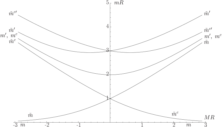
Figure 4: Spectrum of a matter hypermultiplet, in units of $1/R$, as function of $MR$.

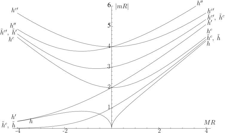
Figure 5: As in Fig. 4 for the Higgs hypermultiplet.

A few things are useful to note. In the large $MR$ limit a supersymmetric spectrum is restored with bound states localized at the boundaries. In Fig. 5 the lightest state which passes through zero at vanishing $MR$ is the Higgs, with the cusp at $MR=0$ reflecting the change of sign of the squared mass, being $\left(m_{h}R\right)^{2}\simeq\frac{4}{\pi}MR$ at $\left|MR\right|\ll 1$.

4 Electroweak symmetry breaking in detail

The purpose of this Section is to study in detail the possible effects of hypermultiplet masses on EWSB. In this paper we consider the case that these masses do not exceed $1/R$, leaving the exploration of the alternative possibility to a future publication. As seen in Sect. 3, moderate values of $MR$ are consistent with radiative corrections. Other than the modification of the spectrum, hypermultiplet masses have 3 types of effects on the EWSB:

1. a mass term for the top $Q$ or $U$ hypermultiplets changes the relation between the top mass and the top-Higgs coupling, crucial in EWSB;

2. a mass term for the top $Q$ or $U$ hypermultiplets influences the one loop Higgs mass or the complete one loop effective potential;

3. a mass term for the Higgs hypermultiplet gives a tree level mass to the zero mode Higgs field (see Fig. 5), which feeds directly in the effective potential.

4.1 The top mass and the top Yukawa coupling

The relation between the top mass and the top–Higgs coupling $y_{t}$ is obtained by solving the equation of motion for the lowest mode of the fermions in the top hypermultiplets $Q$ and $U$, coupled by (3) at the $y=0$ boundary. The interaction (3) is itself a localized mass term when the Higgs scalar is replaced by the vacuum expectation value $v$. This is done in Appendix A. The result can be expressed as

$$y_{t}=\widehat{y}_{t}\eta^{U}_{0}\eta^{Q}_{0}\eta^{h}_{0}$$ (18)

where

$$\widehat{y}_{t} =\frac{\lambda_{t}}{\left(2\pi R\right)^{3/2}}=\frac{2m_{t}}{\pi v}\frac{1}{\sqrt{\omega_{-}^{U}\omega_{-}^{Q}}}$$ (19)

$$\omega_{\pm}^{i} =k_{i}R\coth\left(\frac{k_{i}\pi R}{2}\right)\pm M_{i}R,\ \ \ \ \ \ \ i=U,Q$$ (20)

$$k_{i} =\left(M_{i}^{2}-m_{t}^{2}\right)^{1/2}$$ (21)

and $\eta^{U,Q,h}_{0}$ are the wave functions for the lightest $U,Q,h$ modes at $y=0$, normalized to $\int_{0}^{2\pi R}\textrm{d}y\left|\eta^{i}(y)\right|^{2}=2\pi R$ and given in Appendix A. At $M_{U}=M_{Q}=M_{h}=0$, (18) reduces to

$$y_{t}=\frac{m_{t}}{v}\frac{2\sin\left(\pi Rm_{t}\right)}{\pi Rm_{t}+\sin\left(\pi Rm_{t}\right)}$$ (22)

Note that in the limit $M_{h}=0$, $\left|M_{U,Q}\right|\gg 1/R\gg m_{t}$, $y_{t}$ reduces to the standard value, $m_{t}/v$, no matter what the sign of $M$ is. For positive $M$, when the top wave function and the Yukawa coupling are localized at opposite boundaries, this is due to a compensating increase of $\widehat{y}_{t}$, which is directly related to the fundamental coupling in the Lagrangian. When $y_{t}$ and $\widehat{y}_{t}$ differ significantly, it is $\widehat{y}_{t}$ that enters into (6)-(7) to determine the point of saturation of perturbation theory.

4.2 One loop Higgs effective potential for arbitrary $M_{U}$, $M_{Q}$

The one loop Higgs mass $\left(\ref{eq:corr-m2-result}\right)$ from the diagrams of Fig. 3 gets corrected by the presence of $M_{U}$ and $M_{Q}$. This is in fact also true for the entire one loop effective potential which has to be computed anyhow because of the large correction to the quartic coupling and because of the higher order terms in $\left(vR\right)^{2}$ which may be important insofar as $R$ is not determined.

The calculation described in Sect. 2 immediately generalizes to the massive case in terms of the propagators in presence of masses. Considering, as in $\left(\ref{eq:corr-m2}\right)$, the mixed propagators at $y=y^{\prime}=0$ the effective potential due to top–stop exchanges is

$$V_{t}\left(h;M_{U},M_{Q}\right)= \frac{N_{c}}{2}\sum_{N=1}^{\infty}\int\frac{d^{4}p}{\left(2\pi\right)^{4}}\frac{(-1)^{N+1}}{N}\left(\frac{\lambda_{t}\,h\,\eta_{0}^{h}}{2\sqrt{2\pi R}}\right)^{2N}$$

$$\left\{\left[G_{\varphi}^{U}\left(p,0\right)G_{F}^{Q}\left(p,0\right)\right]^{N}+\left[G_{\varphi}^{Q}\left(p,0\right)G_{F}^{U}\left(p,0\right)\right]^{N}-\,2\left[G_{\psi}^{U}\left(p,0\right)G_{\psi}^{Q}\left(p,0\right)\right]^{N}\right\}$$ (23)

where $G^{U,Q}_{i}\left(p,y\right)=G_{i}\left(p,y;M_{U,Q}\right)$ with $i=\phi,\,F,\,\psi$. The propagators $G_{i}\left(p,y;M\right)$ are given in Appendix B, while the wave function of the Higgs zero mode $\eta_{0}^{h}$ is given in Appendix A.

4.3 Electroweak symmetry breaking in presence of a FI term

As shown in Sect. 3.3, a FI term is equivalent for any hypermultiplet of hypercharge $Y$ to a mass term, which we parameterize in terms of a dimensionless variable $a$ as

$$M\left(Y\right)=\frac{a}{R}Y,$$ (24)

to be inserted in (10,11).

In presence of these masses the potential we consider to determine the VEV of the Higgs field is

$$V\left(h;R,a\right) =m^{2}\left(M\left(1/2\right)\right)h^{2}+\frac{21\xi\left(3\right)}{16\pi^{4}}\frac{g^{2}}{R^{2}}h^{2}$$

$$+\frac{g^{2}+g^{\prime 2}}{8}h^{4}+V_{t}\left(h;M\left(-2/3\right),M\left(1/6\right)\right)$$ (25)

Other than the standard tree-level quartic coupling and the one loop contribution from the top-stop exchanges, eq. $\left(\ref{potenzialeeffettivo}\right)$, the potential includes the tree level mass $m(M)$ computed in Sect. 3.4 and Appendix A (first term on the r.h.s. of (25)) and a one loop mass term from the KK tower of the $SU(2)$ gauge multiplets (second term on the r.h.s. of (25))[15].

Figure 6: Higgs mass as function of the dimensionless parameter $a$, eq. (24).

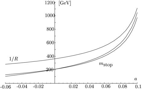
Figure 7: Compactification scale and lightest stop masses as functions of $a$, eq. (24).

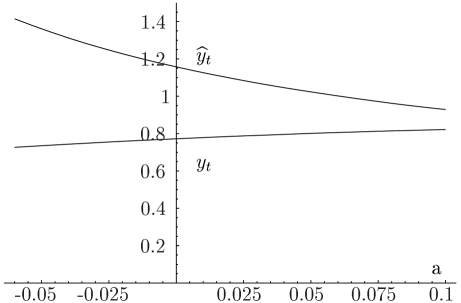
Figure 8: Top–Higgs coupling ($y_{t}$) and $\widehat{y}_{t}=\lambda_{t}/(2\pi R)^{3/2}$ as functions of $a$, eq. (24).

Imposing the occurrence of the minimum at $h=v=175$ GeV determines the Higgs mass $m_{h}$ and $1/R$, together with the entire spectrum, as functions of $a$. The Higgs mass is shown in Fig. 6. The lightest stops, which are non degenerate when $a\neq 0$ because $M_{U}\neq M_{Q}$, occurs in two chiralities. Their mass difference depends on the parameter $a$ and is about $70\,\mbox{{\rm GeV}}$ at $a=0.1$. The stop masses together with $1/R$ are shown in Fig. 7. These figures refine those of Ref. [4].

The sharp increase of $1/R$ with $a$ is due to an increasingly precise accidental cancellation (at about $10\%$ level for $a=0.1$) between the positive tree level squared mass in (25) and the negative contribution from the top-stop loop. Note that the estimate of the radiatively induced FI term in $\left(\ref{massafi}\right)$ corresponds to a negligibly small $a=5\cdot 10^{-3}$ [4].

Through $R$, $M_{U}$ and $M_{Q}$, also the Higgs–top coupling acquires a dependence on $a$, determined in eq. $\left(\ref{eq:uaiti2}\right)$ and shown in Fig. 8. Note that the top Yukawa coupling $y_{t}$ is reduced from the Standard Model value by about $10\%$ due to the localization of the interaction at the boundary.

4.4 Electroweak symmetry breaking with sizeable $M_{U}=M_{Q}$

As we have seen, the mass terms from the FI term have to be small. Their effect can however be significant due to a possible cancellation occurring in the Higgs potential between the tree level Higgs squared mass and the radiatively induced effect. Here we consider the possible effects of direct masses for the $U,Q$ hypermultiplets, taking $M_{U}=M_{Q}=M$ for simplicity. At the same time, again for simplicity, we set the FI term, or the $a$ parameter, to zero.

Proceeding as in the previous section, the Higgs potential we consider is

$$V\left(h;R,M\right)=\frac{21\xi\left(3\right)}{16\pi^{4}}\frac{g^{2}}{R^{2}}h^{2}+\frac{g^{2}+g^{\prime 2}}{8}h^{4}+V_{t}\left(h;M,M\right)$$ (26)

whose minimization determines $m_{h}$ and $R$ as functions of $M.$ The Higgs mass is shown in Fig. 9 for $-0.4\leq MR\leq 0.1$. The reason for interrupting $MR$ below $0.1$ is that the mass of lightest stops falls below the experimental lower bound of about $150$ GeV, as shown in Fig. 10. For $MR$ below $-0.4$, instead, it is the Higgs boson which becomes too light. This result, however, could not persist for $MR<-1$, where higher-loop gauge corrections become important [16]. This case will be analyzed elsewhere. In the interval $-0.4\leq MR\leq 0.1$, both $1/R$ and $m_{\tilde{t}}$ have a non negligible dependence an $M$, as shown in Fig. 10. The degeneracy between the two lightest stop masses would be resolved by taking $M_{U}\neq M_{Q}$. The Top-Higgs couplings $y_{t}$ and $\widehat{y}_{t}$ in this case are shown in Fig. 11.

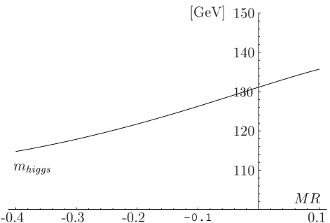
Figure 9: Higgs mass as function of $MR$.

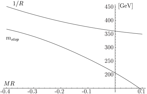
Figure 10: Stop mass and 1/R as functions of $MR$.

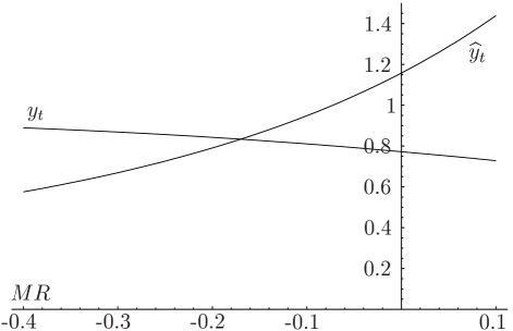
Figure 11: Top-Higgs coupling $y_{t}$ and $\widehat{y}_{t}=\lambda_{t}/(2\pi R)^{3/2}$ as functions of $MR$.

5 Spectrum and phenomenological implications

In absence of hypermultiplet mass terms, the value of the compactification scale and the spectrum of the lightest particles is given in Table 2 with an error that estimates the uncertainties due to the presence of the extra couplings and operators mentioned in Sect. 2.1 [2].

	A	B
$1/R$	$360\pm 70$	$300\div 1000$
$h$	$133\pm 10$	Fig. 12
$\tilde{t}_{1},\,\tilde{u}_{1}$	$210\pm 20$	$1/R(1\pm 8\%)-m_{t}$
$\chi^{\pm},\,\chi^{0},$
$\tilde{g},\,\tilde{q},\,\tilde{l}$	$360\pm 70$	$1/R(1\pm 20\%)$
$\tilde{t}_{2},\,\tilde{u}_{2}$	$540\pm 30$	$1/R(1\pm 8\%)+m_{t}$
$A_{1},q_{1},l_{1},h_{1}$	$720\pm 140$	$2/R(1\pm 20\%)$

Table 2: The particle spectrum and $1/R$ in absence of any mass term (Column A) and in presence of a FI term (Column B). All entries are in GeV.

By letting the mass terms vary in a moderate range, well consistent with radiative corrections, the main deviation from the massless case is due to a possible mass term for the Higgs hypermultiplet which can partially counteract the top-stop radiative corrections that trigger EWSB. This can in turn drive up the compactification scale and, consequently, the entire spectrum.

In Sect. 4.3 we have explicitly discussed the effects of a FI term, which is a particular example of this case. The entire spectrum becomes therefore effectively determined by $1/R$ in the range of Fig. 7, $300\mbox{{\rm GeV}}\lesssim R^{-1}\lesssim 1000\mbox{{\rm GeV}}$. The dependence of $m_{h}$ on $1/R$ is shown in Fig. 12 obtained from Fig. 6–7, whereas the masses of the other particles is again given in Table 2. Note that the lightest stop $\widetilde{t}_{1}$ is the Lightest Supersymmetric Particle (LSP), except possibly for large values of $1/R$ where the corrections due to kinetic terms localized on the boundaries, giving rise to the main uncertainty indicated in Table 2, could reverse the order with any of the other superpartners at $1/R.$ Unless an explicit violation of the $U(1)_{R}$–symmetry were introduced at the boundaries, the LSP would be stable. A moderate effect could also arise from an explicit mass term for the top hypermultiplets, as shown in Fig. 10.

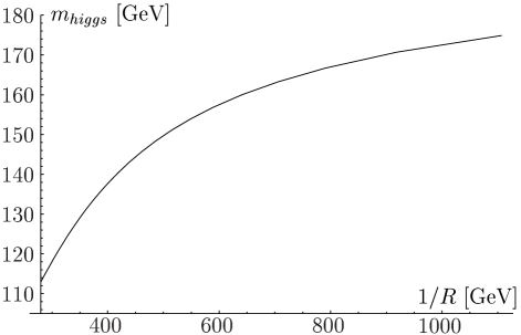
Figure 12: Higgs mass versus $1/R$ in presence of a Fayet-Iliopoulos term.

5.1 Phenomenological implications

Except for the large, somewhat fine tuned values of $1/R,$ the Higgs boson is below the $WW$ threshold, with a preferred mass in the 130 GeV range. It has SM-like couplings to $b\overline{b}$ and $\tau\overline{\tau}$ and $WWh,$ $ZZh$ gauge couplings. It could therefore be looked at in associated production of $Wh$ or $Zh$, followed by $b\overline{b}$ and $\tau\overline{\tau}$ decays. We have already mentioned the deviation of the top Yukawa coupling from the SM value (see Figs. 8, 11). More important for the possible discovery in a hadron collider is the suppression of the Higgs–gluon–gluon squared coupling, ranging from $10\%$ to $60\%$ relative to the SM value as $1/R$ increases from 300 to about 700 GeV, where the $WW$ threshold is crossed [17].

A main feature of the model is that the two degenerate light stops are the LSP and are stable if $U(1)_{R}$ is exact. Their mass is approximately $\left(1/R-m_{t}\right)$ with a lowest preferred value in the 200 GeV range. In such a low range value the super-hadrons $T^{+}=\widetilde{t}_{1}\overline{d}$ and $T^{0}=\widetilde{t}_{1}\overline{u}$ and their charge conjugates $T^{-},\overline{T}^{0}$ could easily be detected at the Tevatron Run II as stable particles, since their possible decay into one another is slow enough to let them both cross the detector. $T^{\pm}$ could appear as a stiff charge track with little hadron calorimeter activity, hitting the muon chambers and distinguishable from a muon via d$E/$d$x$ and time-of-flight. The neutral states, on the contrary, could be identified as missing energy since they could traverse the detector with little interaction. The cross section for the pair production at the Tevatron of the stops with a 200 GeV mass is $0.6$ pb [18].

The heavier supersymmetric particles in Table 2 could be looked at through their chain decay into the LSP. Similarly the discovery of the first states at $2/R$ of the KK tower of SM particles (heavy quarks, leptons with their mirror partners, heavy gauge and Higgs bosons) would be strong evidence for the picture of EWSB described in this paper. Note that (discrete) momentum conservation in the 5th dimension forbids unsuppressed gauge couplings of the heavy gauge bosons to the standard fermions.

Appendices

Appendix A Spectrum

In this appendix we calculate the KK spectrum of Higgs and matter hypermultiplets in presence of a mass term $M$ as in $\left(\ref{eq:lagrangian-mass}\right)$.

Let $\left(\varphi,\psi,F\right)$ ,$\left(\varphi^{c},\psi^{c},F^{c}\right)$ be either a Higgs or a matter hypermultiplet. In presence of a mass term as in $\left(\ref{eq:lagrangian-mass}\right)$ the Lagrangian upon eliminating the F-terms is:

$$\mathcal{L} =\left|\partial_{M}\varphi\right|^{2}+\left|\partial_{M}\varphi^{c}\right|^{2}+i\psi\sigma^{\mu}\partial_{\mu}\overline{\psi}+i\psi^{c}\sigma^{\mu}\partial_{\mu}\overline{\psi}^{c}+\psi^{c}\partial_{y}\psi+\overline{\psi}^{c}\partial_{y}\overline{\psi}$$

$$-M^{2}\left(\left|\varphi\right|^{2}+\left|\varphi^{c}\right|^{2}\right)-2M\left(\delta\left(y\right)+\delta\left(y-\frac{\pi R}{2}\right)\right)\left(\left|\varphi\right|^{2}-\left|\varphi^{c}\right|^{2}\right)$$

$$-M\eta\left(y\right)\left(\psi\psi^{c}+\overline{\psi}\;\overline{\psi}^{c}\right)$$ (27)

where $M=0,1,2,3,5$ while $\mu=0,1,2,3.$

Thus the equations of motion are

$$\left[\partial_{M}\partial^{M}+M^{2}+2M\left(\delta\left(y\right)+\delta\left(y-\frac{\pi R}{2}\right)\right)\right]\varphi=0$$ (28a)

$$\left[\partial_{M}\partial^{M}+M^{2}-2M\left(\delta\left(y\right)+\delta\left(y-\frac{\pi R}{2}\right)\right)\right]\varphi^{c}=0$$ (28b)

$$\left[\partial_{M}\partial^{M}+M^{2}+2M\left(\delta\left(y\right)-\delta\left(y-\frac{\pi R}{2}\right)\right)\right]\psi=0$$ (28c)

$$\left[\partial_{M}\partial^{M}+M^{2}-2M\left(\delta\left(y\right)-\delta\left(y-\frac{\pi R}{2}\right)\right)\right]\psi^{c}=0$$ (28d)

Equations $\left(\ref{eq:equazionidelmoto}\right)$ must be solved imposing the proper boundary conditions to the fields $\varphi$, $\varphi^{c}$, $\psi$, $\psi^{c}$. Note that the delta functions in the left-hand side of equations $\left(\ref{eq:equazionidelmoto}\right)$ are both present only if the field under consideration has $\left(+,+\right)$ parity under $Z_{2}\times Z_{2}^{\prime}$ symmetry. In all other cases the wave function vanishes at $y=0$ and/or $y=\frac{\pi R}{2}$ and the delta functions in the corresponding points are irrelevant.

A.1 Matter hypermultiplets

If we consider a matter hypermultiplet, then $\left(\ref{eq:equazionidelmoto}\right)$ become

$$\left[\partial_{M}\partial^{M}+M^{2}+2M\left(\delta\left(y\right)-\delta\left(y-\frac{\pi R}{2}\right)\right)\right]\psi=0$$ (29a)

$$\left[\partial_{M}\partial^{M}+M^{2}\right]\psi^{c}=0$$ (29b)

$$\left[\partial_{M}\partial^{M}+M^{2}+2M\delta\left(y\right)\right]\varphi=0$$ (29c)

$$\left[\partial_{M}\partial^{M}+M^{2}-2M\delta\left(y-\frac{\pi R}{2}\right)\right]\varphi^{c}=0$$ (29d)

Taking for the wave functions the following form

$$\psi\left(x,y\right)=\left\{\begin{array}[l]{l}\widetilde{\psi}\left(x\right)\left[A_{\psi}\sin k\left(y-\frac{\pi R}{2}\right)+B_{\psi}\cos k\left(y-\frac{\pi R}{2}\right)\right]\\ \widetilde{\psi}\left(x\right)\left[-A_{\psi}\sin k\left(y-\frac{\pi R}{2}\right)+B_{\psi}\cos k\left(y-\frac{\pi R}{2}\right)\right]\end{array}\right.\begin{array}[c]{l}y\in\left(0,\frac{\pi R}{2}\right)\\ y\in\left(\frac{\pi R}{2},\pi R\right)\end{array}$$ (30e)

$$\psi^{c}\left(x,y\right)=\widetilde{\psi}^{c}\left(x\right)A_{\psi^{c}}\sin ky\hskip 169.86298pty\in\left(0,\pi R\right)$$ (30f)

$$\varphi\left(x,y\right)=\widetilde{\varphi}\left(x\right)A_{\varphi}\sin k\left(y-\frac{\pi R}{2}\right)\hskip 131.45158pty\in\left(0,\pi R\right)$$ (30g)

$$\varphi^{c}\left(x,y\right)=\widetilde{\varphi}^{c}\left(x\right)\left\{\begin{array}[l]{l}A_{\varphi^{c}}\sin ky\\ B_{\varphi^{c}}\sin k\left(\pi R-y\right)\end{array}\right.\hskip 102.43008pt\begin{array}[l]{l}y\in\left(0,\frac{\pi R}{2}\right)\\ y\in\left(\frac{\pi R}{2},\pi R\right)\end{array}$$ (30l)

the mass of every field is given by $m^{2}=M^{2}+k^{2}$ where $k$ is constrained by equations $\left(\ref{eq:equazionimotomateria}\right).$ Imposing the proper conditions on the wave functions and their first derivatives on the boundary we get the following equations for $k$

$$\psi\left(+,+\right) \Longrightarrow\left(k^{2}+M^{2}\right)\sin\frac{k\pi R}{2}=0$$ (31a)

$$\psi^{c}\left(-,-\right) \Longrightarrow\sin\frac{k\pi R}{2}=0$$ (31b)

$$\varphi\left(+,-\right) \Longrightarrow\tan\frac{k\pi R}{2}=-\frac{k}{M}$$ (31c)

$$\varphi^{c}\left(-,+\right) \Longrightarrow\tan\frac{k\pi R}{2}=\frac{k}{M}$$ (31d)

A few things are worthy noticing:

1. One can get the equations for the bound states by analytical continuation, setting $k=i\rho$ in $\left(\ref{eq:equazionimateria}\right)$

2. The bound state $\psi\left(+,+\right)$ is massless for every value of $M$, while the excited states have masses $\left(m_{\psi}^{2}\right)_{n}=M^{2}+\left(\frac{2n}{R}\right)^{2},\ n=1,2,\ldots$

3. The equation for $\psi^{c}\left(-,-\right)$ is unaffected by the presence of $M$ because of the vanishing of the wave function at $y=0,\frac{\pi R}{2}$

A.2 Higgs hypermultiplet

If we consider a Higgs hypermultiplet, then $\left(\ref{eq:equazionidelmoto}\right)$ become

$$\left[\partial_{M}\partial^{M}+M^{2}+2M\left(\delta\left(y\right)+\delta\left(y-\frac{\pi R}{2}\right)\right)\right]h=0$$ (32a)

$$\left[\partial_{M}\partial^{M}+M^{2}\right]h^{c}=0$$ (32b)

$$\left[\partial_{M}\partial^{M}+M^{2}+2M\delta\left(y\right)\right]\lambda=0$$ (32c)

$$\left[\partial_{M}\partial^{M}+M^{2}+2M\delta\left(y-\frac{\pi R}{2}\right)\right]\lambda^{c}=0$$ (32d)

With the same procedure of the matter case one gets the equations

$$h\left(+,+\right) \Longrightarrow\tan\frac{k\pi R}{2}=\frac{2kM}{k^{2}-M^{2}}$$ (33a)

$$h^{c}\left(-,-\right) \Longrightarrow\sin\frac{k\pi R}{2}=0$$ (33b)

$$\lambda\left(+,-\right) \Longrightarrow\tan\frac{k\pi R}{2}=-\frac{k}{M}$$ (33c)

$$\lambda^{c}\left(-,+\right) \Longrightarrow\tan\frac{k\pi R}{2}=-\frac{k}{M}$$ (33d)

Note that equation (33a) for the bound state of the $h$ field leads to a negative squared mass if $M<0.$

Solving $\left(\ref{eq:equazionemotohiggsscalare}\right)$ for the zero mode of the Higgs scalar we find for the wave function normalized to $\int_{0}^{2\pi R}\textrm{d}y\left|h^{\left(0\right)}\left(y\right)\right|^{2}=1$

$$h^{\left(0\right)}\left(y\right)=\frac{-k\cos k\left(y-\frac{\pi R}{2}\right)+M\sin k\left(y-\frac{\pi R}{2}\right)}{\sqrt{2M+\left(k^{2}+M^{2}\right)\pi R-2M\cos k\pi R+\left(k-\frac{M^{2}}{k}\right)\sin k\pi R}}$$ (34)

with $k$ the solution of $\left(\ref{eq:equazionehiggsscalare}\right).$ Expression (34) is valid for $y\in\left[0,\pi R/2\right)$. Note that if $M\rightarrow 0,$ then $h^{\left(0\right)}\left(y\right)\rightarrow\left(2\pi R\right)^{-1/2}.$

A.3 Spectrum in presence of a VEV for the Higgs field

If we have a top quark hypermultiplet, then the top Yukawa coupling

$$\mathcal{L}_{Y}=\frac{\lambda_{t}}{2}\left[\delta\left(y\right)+\delta\left(y-\pi R\right)\right]\int\text{d}^{2}\theta\widehat{h}\,\widehat{Q}\,\widehat{U}+\textrm{h.c.}$$ (35)

leads to a mass term when we replace the Higgs zero mode $h^{\left(0\right)}$ with its VEV $v.$ To calculate the spectrum in presence of such a term it is convenient to rewrite the Lagrangian $\left(\ref{eq:lagrangiana}\right)$ without eliminating the $F$ auxiliary fields and use the following vectors

$$\begin{array}[]{ccc}X=\left(\begin{array}[]{c}\varphi\\ F^{c\dagger}\end{array}\right)&Y=\left(\begin{array}[]{c}\varphi^{c}\\ F^{\dagger}\end{array}\right)&Z=\left(\begin{array}[]{c}\psi\\ \bar{\psi^{c}}\end{array}\right)\end{array}$$ (36)

Then $\left(\ref{eq:lagrangiana}\right)$ becomes

$$\mathcal{L} =\left(\begin{array}[c]{cc}X_{U,Q}^{\dagger}&Y_{Q,U}^{\dagger}\end{array}\right)M_{B}\left(\begin{array}[c]{c}X_{U,Q}\\ Y_{Q,U}\end{array}\right)$$ (40)

$$+\left(\begin{array}[c]{cc}\overline{Z}_{U,Q}&Z^{t}_{Q,U}\end{array}\right)M_{F}\left(\begin{array}[c]{c}Z_{U,Q}\\ \overline{Z}^{t}_{Q,U}\\ \end{array}\right)$$ (44)

where

$$M_{B}=\left(\begin{array}[c]{cccc}-\square-4M_{U,Q}\delta_{\pi R/2}&\partial_{y}+\eta\left(y\right)M_{U,Q}&0&\lambda_{t}\alpha^{*}\\ -\partial_{y}+\eta\left(y\right)M_{U,Q}&1&0&0\\ 0&0&-\square+4M_{Q,U}\delta_{\pi R/2}&-\partial_{y}+\eta\left(y\right)M_{Q,U}\\ \lambda_{t}\alpha&0&\partial_{y}+\eta\left(y\right)M_{Q,U}&1\end{array}\right)$$ (45e)

$$M_{F}=\left(\begin{array}[c]{cccc}\partial_{y}-\eta\left(y\right)M_{U,Q}&i\sigma^{\mu}\partial_{\mu}&0&0\\ i\overline{\sigma}^{\mu}\partial_{\mu}&-\partial_{y}-\eta\left(y\right)M_{U,Q}&0&\lambda_{t}\alpha^{*}\\ \lambda_{t}\alpha&0&-\partial_{y}-\eta\left(y\right)M_{U,Q}&i\sigma^{\mu}\partial_{\mu}\\ 0&0&i\overline{\sigma}^{\mu}\partial_{\mu}&\partial_{y}-\eta\left(y\right)M_{U,Q}\end{array}\right)$$ (45j)

$$\begin{array}[]{lcr}\alpha=\frac{1}{2}\left[\delta\left(y\right)+\delta\left(y-\pi R\right)\right]v\;h^{\left(0\right)}\left(y=0\right),&&\delta_{\pi R/2}=\delta\left(y-\frac{\pi R}{2}\right)\end{array}$$

with $h^{\left(0\right)}\left(y=0\right)$ the Higgs zero mode wave function (34) at $y=0.$

Taking for the wave functions the form $\left(\ref{eq:funzionid'onda}\right)$ (in this case one must consider also the wave functions of $F_{U,Q},F_{Q,U}^{c}$) and imposing the proper boundary conditions one can get the equations for the masses of the fields $\varphi_{U,Q},\psi_{U,Q},\varphi_{U,Q}^{c},\psi_{U,Q}^{c}.$

For the top quark $\psi_{U,Q}$ and the top squark $\varphi_{U,Q}$ (the lowest modes) one gets

$$m_{t}^{2}=\frac{\lambda_{t}^{2}v^{2}\left|h^{\left(0\right)}\left(0\right)\right|^{2}}{16}\left(k_{U}^{t}\coth\frac{k_{U}^{t}\pi R}{2}-M_{U}\right)\left(k_{Q}^{t}\coth\frac{k_{Q}^{t}\pi R}{2}-M_{Q}\right)$$ (46)

$$\left(k_{U}^{\tilde{t}}\coth\frac{k_{U}^{\tilde{t}}\pi R}{2}+M_{U}\right)\left(k_{Q}^{\tilde{t}}\coth\frac{k_{Q}^{\tilde{t}}\pi R}{2}-M_{Q}\right)= \frac{\lambda_{t}^{2}v^{2}\left|h^{\left(0\right)}\left(0\right)\right|^{2}}{16}$$

$$\left(m_{\tilde{t}}^{2}+2M_{Q}\left(k_{Q}^{\tilde{t}}\coth\frac{k_{Q}^{\tilde{t}}\pi R}{2}-M_{Q}\right)\right)$$ (47)

where $k_{U,Q}^{t,\tilde{t}}=\sqrt{M_{U,Q}^{2}-m_{t,\tilde{t}}^{2}}.$ The wave function of the top quark zero mode, normalized to $\int_{0}^{2\pi R}\textrm{d}y\left|\psi_{0}^{U,Q}\left(y\right)\right|^{2}=1$, is obtained by solving equation (29a). For $y\in\left[0,\pi R/2\right)$ we have

$$\psi_{0}^{U,Q}\left(y\right)=\frac{k_{U,Q}\cosh k_{U,Q}\left(\frac{\pi R}{2}-y\right)-M_{U,Q}\sinh k_{U,Q}\left(\frac{\pi R}{2}-y\right)}{\sqrt{-m_{t}^{2}\pi R+2M_{U,Q}\left(-\cosh k_{U,Q}\pi R+1\right)+\left(k_{U,Q}+\frac{M^{2}}{k_{U,Q}}\right)\sinh k_{U,Q}\pi R}}$$ (48)

The usual 4D top Yukawa coupling, defined as the coupling among the zero modes of the fields $h,\psi_{U},\psi_{Q},$ is given by

$$y_{t}=\widehat{y}_{t}\eta_{0}^{h}\eta_{0}^{U}\eta_{0}^{Q}$$ (49)

where $\widehat{y}_{t}=\lambda_{t}\left(2\pi R\right)^{-3/2}$ and $\eta_{0}^{i}$ ($i=h,U,Q$) are the wave functions $\left(\ref{eq:funzioned'ondahiggs}\right)-\left(\ref{eq:funzioned'ondatop}\right)$ at $y=0$ normalized in such a way that

$$\int_{0}^{2\pi R}\textrm{d}y\left|\eta^{i}_{0}\left(y\right)\right|^{2}=2\pi R$$ (50)

Inserting (49) into (46) we obtain the relation between the top quark mass $m_{t}$ and the 4D Yukawa coupling $y_{t}$.

Appendix B Propagators

In order to obtain the mixed momentum–coordinate space propagators for the components $\varphi$, $\psi$, $F$ of a hypermultiplet, we start from the 5D Lagrangian without eliminating the auxiliary fields. If $M\neq 0$ the relevant part of this Lagrangian is:

$${\cal L}= \left|\partial_{\mu}\varphi\right|^{2}+\left|\partial_{\mu}\varphi^{c}\right|^{2}+\left|F\right|^{2}+\left|F^{c}\right|^{2}+i\bar{\psi}\bar{\sigma}^{\mu}\partial_{\mu}\psi+i\psi^{c}\sigma^{\mu}\partial_{\mu}\bar{\psi}^{c}+$$

$$+\left[F\partial_{y}\varphi^{c}-F^{c}\partial_{y}\varphi+\mbox{{\rm h.\,c.}}\right]+M\eta(y)\left[F\varphi^{c}+F^{c}\varphi+\mbox{{\rm h.\,c.}}\right]$$

$$+\left[\psi^{c}\partial_{y}\psi+\mbox{{\rm h.\,c.}}\right]-M\eta(y)\left[\psi^{c}\psi+\mbox{{\rm h.\,c.}}\right]$$

$$-4M\delta(y-\pi R/2)\left[\left|h\right|^{2}-\left|h^{c}\right|^{2}\right]$$ (51)

for the generic hypermultiplet of components $\varphi$, $\psi$, $F$ and their conjugates. The border term at $\pi R/2$ in the last line is necessary to maintain 5D SUSY invariance under $\xi^{-+}$ transformations. In this paper we need only the propagators for the top–stop sector, so we can assume from now on that the parities are those of the matter multiplets. Using the vectors defined in (36), $\mathcal{L}$ can be recast in a more compact form as in Appendix A:

$${\cal L}=X^{\dagger}AX+Y^{\dagger}BY+\bar{Z}CZ$$ (52)

where

$$\begin{array}[]{cc}A=\left(\begin{array}[]{cc}-\square-4M\delta(y-\pi R/2)&\partial_{y}+M\eta(y)\\ -\partial_{y}+M\eta(y)&1\end{array}\right)&B=\left(\begin{array}[]{cc}-\square+4M\delta(y-\pi R/2)&-\partial_{y}+M\eta(y)\\ \partial_{y}+M\eta(y)&1\end{array}\right)\end{array}$$ (58)

$$C=\left(\begin{array}[]{cc}\partial_{y}-M\eta(y)&i\sigma^{\mu}\partial_{\mu}\\ i\bar{\sigma}^{\mu}\partial_{\mu}&-\partial_{y}-M\eta(y)\end{array}\right)$$ (61)

Note that the components of $X$ (or $Y$, $Z$) have the same quantum numbers but different boundary conditions.

Let us focus, for example, on the propagator

$$G\left[(x-x^{\prime})_{\mu};y,y^{\prime}\right]=\langle\varphi(x_{\mu}^{\prime},y^{\prime})\varphi^{\dagger}(x_{\mu},y)\rangle,$$ (62)

the others being analogous. In general all the correlation functions will depend on both $y$ and $y^{\prime}$ because of the non conservation of the 5th component of momentum in the segment $[0,\pi R/2]$. However, being interested in calculating only loops formed using Yukawa interactions which are localized at $y=0$, we can impose without any problem $y^{\prime}=0$ from the very beginning of the calculation, reducing the dependence of the (62) only to $(x-x^{\prime})_{\mu}$ and $y$.

One can arrange propagators in matrices using the vectors previously defined. In particular, defining

$${\cal G}(x-x^{\prime};y) = \langle X(x,y)X^{\dagger}(x^{\prime},0)\rangle$$ (65)

$$= \left(\begin{array}[]{cc}\langle\varphi(x,y)\varphi^{\dagger}(x^{\prime},0)\rangle&\langle\varphi(x,y)F^{c}(x^{\prime},0)\rangle\\ \langle F^{c\dagger}(x,y)\varphi^{\dagger}(x^{\prime},0)\rangle&\langle F^{c\dagger}(x,y)F^{c}(x^{\prime},0)\rangle\end{array}\right)$$

the equations of motion for the scalar Green functions are:

$$A{\cal G}(x-x^{\prime};y)=i\delta^{(4)}(x-x^{\prime})\delta(y)$$ (66)

Multiplying the 1st row of $A$ by the 1st column of $\mathcal{G}$ we get a system of 2 differential equations, which after passing to euclidian 4-momentum, assumes the form:

$$\left\{\begin{array}[]{l}-k_{4}^{2}g(y)-4M\delta(y-\pi R/2)+\left(\partial_{y}+M\eta(y)\right)f(y)=\delta(y)\\ (-\partial_{y}+M\eta(y))g(y)+f(y)=0\end{array}\right.$$

where $g(y)=\langle\varphi(y)\varphi^{\dagger}(0)\rangle$ and $f(y)=\langle F^{c\dagger}(y)\varphi^{\dagger}(0)\rangle$. These coupled equations must be solved imposing the $(+,-)$ and the $(-,+)$ boundary conditions in $y$ on $g$ and $f$ respectively, using the same techniques of Appendix A. One finally gets the $\langle\varphi\varphi^{\dagger}\rangle$ propagator $G_{\varphi}\left(k_{4},y;M\right)$:

$$G_{\varphi}\left(k_{4},y;M\right)=\langle\varphi\varphi^{\dagger}\rangle(y)=\frac{\sinh\left[k\left(\frac{\pi R}{2}-y\right)\right]}{2\left[k\cosh\left(\frac{k\pi R}{2}\right)+M\sinh\left(\frac{k\pi R}{2}\right)\right]}$$ (67)

where $k=\sqrt{k_{4}^{2}+M^{2}}$. Analogously the $\langle FF^{\dagger}\rangle$ $(+,-)$ and $\langle\psi\psi^{\dagger}\rangle$ $(+,+)$ propagators are:

$$G_{F}\left(k_{4},y;M\right)=\frac{k_{4}^{2}}{2}\frac{\sinh\left[k\left(\frac{\pi R}{2}-y\right)\right]}{\left[k\cosh\left(\frac{k\pi R}{2}\right)-M\sinh\left(\frac{k\pi R}{2}\right)\right]}\left(1-\frac{2M}{k_{4}^{2}}\left(k\coth\left(\frac{k\pi R}{2}\right)-M\right)\right)$$

$$G_{\psi}\left(k_{4},y;M\right)=\frac{k\!\!\!\!\diagup_{4}}{2k_{4}^{2}}\frac{k\cosh\left[k\left(\frac{\pi R}{2}-y\right)\right]+M\sinh\left[k\left(\frac{\pi R}{2}-y\right)\right]}{\sinh\left(\frac{k\pi R}{2}\right)}$$ (68)

where $k\!\!\!\!\diagup_{4}=\sigma\cdot k_{4}$.

In the limit $M\rightarrow 0$ these propagators become:

$$G_{\varphi}(k_{4},y;M=0)=\frac{1}{2k_{4}}\frac{\sinh\left[k_{4}\left(\frac{\pi R}{2}-y\right)\right]}{\cosh\left(\frac{k_{4}\pi R}{2}\right)}$$

$$G_{F}(k_{4},y;M=0)=\frac{k_{4}}{2}\frac{\sinh\left[k_{4}\left(\frac{\pi R}{2}-y\right)\right]}{\cosh\left(\frac{k_{4}\pi R}{2}\right)}$$

$$G_{\psi}(k_{4},y;M=0)=\frac{k\!\!\!\!\diagup_{4}}{2k_{4}}\frac{\cosh\left[k_{4}\left(\frac{\pi R}{2}-y\right)\right]}{\sinh\left(\frac{k_{4}\pi R}{2}\right)}$$ (69)

References

- [1] R. Barbieri and A. Strumia, arXiv:hep-ph/0007265.
- [2] R. Barbieri, L. J. Hall and Y. Nomura, Phys. Rev. D 63 (2001) 105007 [arXiv:hep-ph/0011311].
- [3] D. M. Ghilencea, S. Groot Nibbelink and H. P. Nilles, Nucl. Phys. B 619 (2001) 385 [arXiv:hep-th/0108184].
- [4] R. Barbieri, L. J. Hall and Y. Nomura, arXiv:hep-ph/0110102.
- [5] C. A. Scrucca, M. Serone, L. Silvestrini and F. Zwirner, Phys. Lett. B 525 (2002) 169 [arXiv:hep-th/0110073].
- [6] R. Barbieri, R. Contino, P. Creminelli, R. Rattazzi and C. A. Scrucca, arXiv:hep-th/0203039.
- [7] N. Arkani-Hamed, L. J. Hall, Y. Nomura, D. R. Smith and N. Weiner, Nucl. Phys. B 605 (2001) 81 [arXiv:hep-ph/0102090].
- [8] Z. Chacko, M. A. Luty and E. Ponton, JHEP 0007 (2000) 036 [arXiv:hep-ph/9909248].
- [9] R. Barbieri, L. J. Hall and Y. Nomura, Nucl. Phys. B 624 (2002) 63 [arXiv:hep-th/0107004].
- [10] N. Arkani-Hamed, A. G. Cohen and H. Georgi, Phys. Lett. B 516 (2001) 395 [arXiv:hep-th/0103135].
- [11] L. Pilo and A. Riotto, arXiv:hep-th/0202144.
- [12] R. Barbieri, S. Ferrara, D. V. Nanopoulos and K. S. Stelle, Phys. Lett. B 113 (1982) 219.
- [13] S. Ferrara, L. Girardello, T. Kugo and A. Van Proeyen, Nucl. Phys. B 223 (1983) 191.
- [14] E. A. Mirabelli and M. E. Peskin, Phys. Rev. D 58 (1998) 065002 [arXiv:hep-th/9712214].
- [15] I. Antoniadis, S. Dimopoulos, A. Pomarol and M. Quiros, Nucl. Phys. B 544 (1999) 503 [arXiv:hep-ph/9810410].
- [16] D. Marti and A. Pomarol, arXiv:hep-ph/0205034.
- [17] G. Cacciapaglia, M. Cirelli and G. Cristadoro, Phys. Lett. B 531 (2002) 105 [arXiv:hep-ph/0111287].
- [18] M. Chertok, G. D. Kribs, Y. Nomura, W. Orejudos, B. Schumm and S. Su, in Proc. of the APS/DPF/DPB Summer Study on the Future of Particle Physics (Snowmass 2001) ed. R. Davidson and C. Quigg, arXiv:hep-ph/0112001.
- [19] N. Arkani-Hamed, T. Gregoire and J. Wacker, JHEP 0203 (2002) 055 [arXiv:hep-th/0101233].