1 Introduction

CP violation has been observed so far in the neutral K meson system, both in $|\Delta S|=2$ and $|\Delta S|=1$ processes, and recently also in neutral B meson decays. These phenomena are very probably caused by the Kobayashi-Maskawa (KM) mechanism, that is to say by a non-zero phase $\delta_{KM}$ in the coupling matrix of the charged weak quark currents to W bosons. CP violation found so far in these meson systems does not catch the eye: either the value of the CP observable or/and the branching ratio of the associated mesonic decay mode is small. However, the interactions that give rise to these subtle effects may have also been jointly responsible for an enormous phenomenon, namely for the apparent matter-antimatter asymmetry of the universe. In this context it has been a long-standing question whether or not CP violation in $K^{0}-{\bar{K}^{0}}$ mixing, i.e. the parameter $\epsilon_{K}$, is related to the baryon asymmetry of the universe (BAU) $\eta=(n_{b}-n_{\bar{b}})/n_{\gamma}\sim 10^{-10}$. In particular, is the experimental result ${\rm Re}\ \epsilon_{K}>0$ related to the fact that our universe is filled with matter rather than antimatter? Because the CP effects observed so far in $K$ and $B$ meson decays are consistently explained by the KM mechanism, one may paraphrase these questions in more specific terms by asking whether the standard model of particle physics (SM) combined with the standard model of cosmology (SCM) can explain the value of $\eta$? This has been answered in recent years and, surprisingly, the answer does not refer to the role the KM phase $\delta_{KM}$ may play in these explanatory attempts. Theoretical progress in understanding the SM electroweak phase transition in the early universe in conjunction with the experimental lower bound on the mass of the SM Higgs boson, $m_{H}^{SM}>114$ GeV, leads to the conclusion: no! In these lecture notes an introduction is given to concepts and results which are necessary to understand how this conclusion is reached. Furthermore I shall discuss a few viable (so far) and rather plausible baryogenesis scenarios beyond the SM.

The plan of these notes is as follows: Section 2 contains some basics of the SCM which are used in the following chapters. Equilibrium distributions and rough criteria for the departure from local thermal equilibrium are recalled. In section 3 a heuristic discussion of the BAU $\eta$ is given. Then the Sakharov conditions for generating a baryon asymmetry within the SCM are discussed and illustrated. In section 4 we review how baryon number (B) violation occurs in the SM and how strong B-violating SM reaction rates are below and above the electroweak phase transition. Section 5 is devoted to electroweak baryogenesis scenarios. The electroweak phase transition is discussed, including results concerning its nature in the SM which reveal why the SM fails to explain the observed BAU. Nevertheless, electroweak baryogenesis is still a viable scenario in extensions of the SM, for instance in 2-Higgs doublet and supersymmetric (SUSY) extensions. We shall outline this in the context of one of the several non-SM electroweak baryogenesis mechanisms which were developed. In section 6 we discuss the perhaps most plausible, in any case most popular, baryogenesis scenario above the electroweak phase transition, namely the out-of-equilibrium decay of (a) superheavy particle(s). After having recalled a textbook example of baryogenesis in grand unified theories (GUTs), we turn to a viable and attractive scenario that has found much attention in recent years, which is baryogenesis through leptogenesis caused by the decays of heavy Majorana neutrinos. A summary and outlook is given in section 7. Some formulae concerning the transformation properties of the baryon number operator and the properties of Majorana neutrino fields are contained in appendices A and B, respectively.

Throughout these lectures the natural units of particle physics are used in which $\hbar=c=k_{B}=1$, where $k_{B}$ is the Boltzmann constant. In these units we have, for instance, that 1 GeV $\simeq$ $10^{13}K$ and 1$({\rm GeV})^{-1}\simeq 6\times 10^{-25}s$. Moreover, it is useful to recall that the present extension of the visible universe is characterized by the Hubble distance $H_{0}^{-1}\sim 10$ Gpc, where 1 pc $\simeq$ 3.2 light years.

These lectures were intended as an introduction to the subject for graduate students. The reader who wants to delve more deeply into these topics should consult the textbook [1], the reviews [2, 3, 4, 5, 6, 7] and, of course, the original literature.

2 Some Basics of Cosmology

2.1 The Standard Model of Cosmology

The current understanding of the large-scale evolution of our universe is based on a number of observations. These include the expansion of the universe and the approximate isotropic and homogeneous matter and energy distribution on large scales. The Einstein field equations of general relativity imply that the metric of space-time shares these symmetry properties of the sources of gravitation on large scales. It is represented by the Robertson-Walker (RW) metric which corresponds to the line element

$$ds^{2}=dt^{2}-R^{2}(t)\left\{\frac{dr^{2}}{1-kr^{2}}+r^{2}d{\theta}^{2}+r^{2}\sin^{2}\theta\,d\theta d{\phi}^{2}\right\}\>,$$ (1)

where $(t,r,\theta,\phi)$ are the dimensionless comoving coordinates and $k=0,1,-1$ for a space of vanishing, positive, or negative spatial curvature. Cosmological data are consistent with $k=0$ [9]. The dynamical variable $R(t)$ is the cosmic scale factor and has dimension of length. The matter/energy distribution on large scales may be modeled by the stress-energy tensor of a perfect fluid, $T^{\mu}_{\,\nu}=$diag$(\rho,-p,-p,-p)$, where $\rho(t)$ is the total energy density of the matter and radiation in the universe and $p(t)$ is the isotropic pressure.

The dynamical equations which determine the time-evolution of the scale factor follow from Einstein’s equations. Inserting the metric tensor which is encoded in (1) and the above form of $T_{\mu\nu}$ into these equations one obtains the Friedmann equation

$$H^{2}\>\equiv\>\left(\frac{\dot{R}}{R}\right)^{2}\>=\>\frac{8\pi G_{N}}{3}\rho-\frac{k}{R}+\frac{\Lambda}{3}\>.$$ (2)

Here $H(t)\equiv\dot{R}(t)/R(t)$ is the Hubble parameter which measures the expansion rate of the universe at time $t$, and $\Lambda$ denotes the cosmological “constant” at time t. According to the inflationary universe scenario the $\Lambda$ term played a crucial role at a very early epoch when vacuum energy was the dominant form of energy in the universe, leading to an exponential increase of the scale factor. Recent observations indicate that today the largest component of the energy density of the universe is some dark energy which can also be described by a non-zero cosmological constant [9]. The baryogenesis scenarios that we shall discuss in these lecture notes are associated with a period in the evolution of the early universe where, supposedly, a $\Lambda$ term in the evolution equation (2) for $H$ can be neglected.

The covariant conservation of the stress tensor $T_{\mu\nu}$ yields another important equation, namely

$$d(\rho R^{3})=-pd(R^{3})\>.$$ (3)

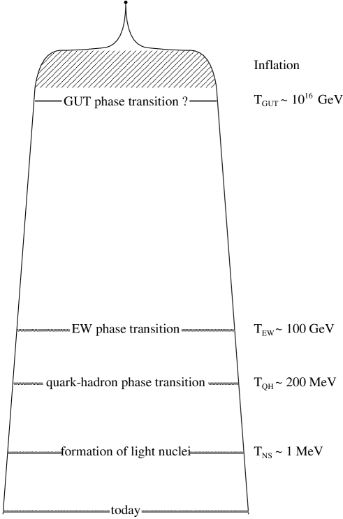
Figure 1: Cartoon of the history of the universe. The slice of a cake, stretched at the top, illustrates the expansion of the universe as it cooled off. Inflation may have ended well below $T_{GUT}$ [6].

This can be read as the first law of thermodynamics: the total change of energy is equal to the work done on the universe, $dU=dA=-pdV$. Moreover, it turns out (see section 2.2) that the various forms of matter/energy which determine the state of the universe during a certain epoch can be described, to a good approximation, by the equation of state

$$p=w\rho\>,$$ (4)

where, for instance, $w=1/3,0,-1$ if the energy of the universe is dominated by relativistic particles (i.e., radiation), non-relativistic particles, and vacuum energy, respectively.

Integrating (3) with (4) one obtains that the energy density evolves as $\rho\propto R^{-3(1+w)}$. In the radiation-dominated era, $\rho\propto R^{-4}$. Inserting this scaling law into the Friedmann equation, one finds that in this epoch the expansion rate behaves as

$$H(t)\propto t^{-1}.$$ (5)

Fig. 1 illustrates the history of the early universe, as reconstructed by the SCM and by the SM of particle physics. The baryogenesis scenarios which will be discussed in sections 5 and 6 apply to some instant in the – tiny – time interval after inflation and before or at the time of the electroweak phase transition. In this era, where the SM particles were massless, the energy of the universe was – according to what is presently known – essentially due to relativistic particles.

2.2 Equilibrium Thermodynamics

As was just mentioned the baryogenesis scenarios which we shall discuss in sections 5 and 6 apply to the era between the end of inflation and the electroweak phase transition. During this period the universe expanded and cooled off to temperatures $T\gtrsim T_{EW}\sim 100$ GeV. For most of the time during this stage the reaction rates of the majority of particles were much faster than the expansion rate of the cosmos. The early universe, which we view as a (dense) plasma of particles, was then to a good approximation in thermal equilibrium. In several situations it is reasonable to treat this gas as dilute and weakly interacting. Let’s therefore recall the equilibrium distributions of an ideal gas. Because particles in the early universe were created and destroyed, it is natural to describe the gas by means of the grand canonical ensemble. Consider an ensemble of a relativistic particle species A. Its phase space distribution or occupancy function is given by

$$f_{A}({\bf p})=\frac{1}{e^{(E_{A}-\mu_{A})/T_{A}}\mp 1}\>,$$ (6)

where $T_{A}$ is the temperature, $\mu_{A}$ is the chemical potential of the species which is associated with a conserved charge of the ensemble, and the minus (plus) sign refers to bosons (fermions). If different species are in chemical equilibrium then their chemical potentials are related. For instance, suppose the particle reaction $A+B\leftrightarrow C$ takes place rapidly. Then the relation $\mu_{A}+\mu_{B}=\mu_{C}$ holds. Take the standard example $e^{+}+e^{-}\leftrightarrow n\gamma$. Because $\mu_{\gamma}=0$ we have $\mu_{e^{+}}=-\mu_{e^{-}}$.

From (6) one obtains the number density $n_{A}$, the energy density $\rho_{A}$, the isotropic pressure $p_{A}$, and the entropy density $s_{A}$. Defining $d{\tilde{p}}\equiv d^{3}p/(2\pi)^{3}$ we have

$$n_{A} = g_{A}\int d{\tilde{p}}\,f_{A}({\bf p})\>,$$ (7)

$$\rho_{A} = g_{A}\int d{\tilde{p}}\>E_{A}({\bf p})f_{A}({\bf p})\,,$$ (8)

$$p_{A} = g_{A}\int d{\tilde{p}}\>\frac{\bf p^{2}}{3E_{A}}f_{A}({\bf p})\,,$$ (9)

$$s_{A} = \frac{\rho_{A}+p_{A}}{T}\,.$$ (10)

Here $E_{A}=\sqrt{{\bf p^{2}}+m_{A}^{2}}$, where $m_{A}$ is the mass of A, and $g_{A}$ denotes the internal degrees of freedom of A; for instance, $g_{e}=2$ for the electron and $g_{\nu}=1$ for a massless neutrino.

In the following we need these expressions in the ultra-relativistic ($T_{A}>>m_{A}$) and nonrelativistic ($T_{A}<<m_{A}$) limits. Integrating eqs. (7) - (9) one obtains the well-known textbook formulae for $n_{A}$, $\rho_{A}$, and $p_{A}$. For relativistic particles A (and $T_{A}>>\mu_{A}$)

$$n_{A} = a_{A}g_{A}T_{A}^{3}\,,$$ (11)

$$\rho_{A} = b_{A}g_{A}T_{A}^{4}\,,$$ (12)

$$p_{A} \simeq \rho_{A}/3\,,$$ (13)

while for nonrelativistic particles the number density becomes exponentially suppressed for decreasing temperature:

$$n_{A} = g_{A}(\frac{m_{A}T_{A}}{2\pi})^{3/2}e^{-(m_{A}-\mu_{A})/T_{A}}\,,$$ (14)

$$\rho_{A} = n_{A}m_{A}\,,$$ (15)

$$p_{A} \simeq n_{A}T_{A}<<\rho_{A}\,.$$ (16)

In eqs. (11), (12) $a_{A}$ and $b_{A}$ are numbers depending on whether A is a boson or fermion. Eqs. (13), (16) are the equations of state that we used already above.

When considering the total energy density and pressure of all particle species it is useful to express these quantities in terms of the photon temperature T. The corresponding formulae are obtained in a straightforward fashion by summing the respective contributions, taking into account that some species A may have a thermal distribution with a temperature $T_{A}\neq T$. When the universe was in thermal equilibrium its entropy remained constant. Its entropy density is given by

$$s=\frac{S}{V}=\frac{\rho+p}{T}=\frac{2\pi^{2}}{45}g_{*s}T^{3}\,,$$ (17)

where the last equality comes from the fact that $s$ is dominated by the contributions from relativistic particles. During the epoch we are interested in, the factor $g_{*s}$ was equal to the total number of relativistic degrees of freedom $g_{*}$ [1]. (For $T>>m_{top}$ we have $g_{*}\simeq 106$ in the SM.) The entropy being constant implies $s\propto R^{-3}$, hence $g_{*s}T^{3}R^{3}=const$. From this we obtain that in the radiation dominated epoch the temperature of the universe decreased as

$$T\propto R^{-1}\,.$$ (18)

From these relations we can draw another important conclusion. Consider the number $N_{A}$ of some particle species A. Because $N_{A}\equiv R^{3}n_{A}\propto n_{A}/s$ this ratio also remained constant, in the absence of “A number” violation and/or entropy production, during the expansion of the universe. Therefore in the context of baryogenesis the relevant quantity is the baryon-to-entropy ratio $n_{B}/s\equiv(n_{b}-n_{\bar{b}})/s$, where $n_{b}$ and $n_{\bar{b}}$ denotes the number density of baryons and antibaryons, respectively. The BAU $\eta\equiv n_{B}/n_{\gamma}$ is given in terms of this ratio by $\eta=1.8g_{*s}n_{B}/s$. The relativistic degrees of freedom $g_{*s}$ decreased during the expansion of the early universe. This number and, hence, $\eta$ remained constant only after the time of $e^{+}e^{-}$ annihilation. From then on

$$\eta\simeq 7\frac{n_{B}}{s}.$$ (19)

2.3 Departures from Thermal Equilibrium

Departures from thermal equilibrium (DTE) were, of course, crucial for the development of the universe to that state that we perceive today. Examples for DTEs include the decoupling of neutrinos, the decoupling of the photon background radiation, and primordial nucleosynthesis. More speculative examples are inflation, first order phase transitions in the early universe (see below), the decoupling of weakly interacting massive particles, and the topic of these lectures, baryogenesis. In any case the DTEs have led to the (light) elements, to a net baryon number of the visible universe, and to the neutrino and the microwave background.

A rough criterion for whether or not a particle species A is in local thermal equilibrium is obtained by comparing reaction rate $\Gamma_{A}$ with the expansion rate $H$. Let $\sigma(A+target\to X)$ be the total cross section of the reaction(s) of A that is (are) crucial for keeping A in thermal equilibrium. Then $\Gamma_{A}$ is given by

$$\Gamma_{A}=\sigma(A+target\to X)n_{target}|{\bf v}|\,,$$ (20)

where $n_{target}$ is the target density and ${\bf v}$ is the relative velocity. Keep in mind that $[\Gamma_{A}]=(sec)^{-1}$. If

$$\Gamma_{A}\gtrsim H\,,$$ (21)

then the reactions involving A occur rapidly enough for A to maintain thermal equilibrium. If

$$\Gamma_{A}<H\,,$$ (22)

then the ensemble of particles A will fall out of equilibrium. The Hubble parameter $H(t)$ which is relevant for the baryogenesis scenarios to be discussed below is the expansion rate during the radiation dominated epoch. It follows from eqs. (2) and (12) that in this era

$$H=\sqrt{\frac{8\pi G_{N}}{3}}\rho=1.66\sqrt{g_{*}}\frac{T^{2}}{m_{Pl}}\,,$$ (23)

where $m_{Pl}=1.22\times 10^{19}$GeV denotes the Planck mass.

Eqs. (21) and (22) constitute a useful rule of thumb that is often quite accurate. It is sufficient for the purpose of these lectures. A proper treatment involves the determination of the time evolution of the particle’s phase space distribution $f_{A}$ which is governed by the Boltzmann equation (cf. for instance [1]). Comparing the number density $n_{A}(t)$, obtained from solving this equation, with the equilibrium distribution $n_{A}^{eq}$ (which was discussed above for (non)relativistic particles) one sees whether or not A has decoupled from the thermal bath. Rather than going into details let us sketch in Fig. 2 the behaviour of the ratio

$$Y_{A}\equiv\frac{n_{A}}{s}$$ (24)

as a function of the decreasing temperature when an ensemble of massive particles A decouples from the thermal bath. In thermal equilibrium $Y_{A}$ is constant for $T>>m_{A}$. At later times, when $T\lesssim m_{A}$, $Y_{A}\propto(m_{A}/T)^{3/2}\exp(-m_{A}/T)$ if the reaction rate still obeys (21). Thus, if A would have remained in thermal equilibrium until today its abundance would be completely negligible. However, if $\Gamma_{A}$ becomes smaller than $H$, the interactions of A “freeze out”, and the actual abundance of A deviates from its equilibrium value at temperature $T$. The larger the $A\bar{A}$ annihilation cross section the smaller the decoupling temperature and the actual abundance $Y_{A}$. The further fate of the decoupled species depends on whether or not A is stable. If a (quasi)stable species A – a weakly interacting massive particle – froze out at a temperature T not much smaller than $m_{A}$ then its abundance today can be significant.

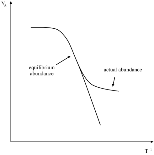
Figure 2: The behaviour of $Y_{A}\equiv{n_{A}}/{s}$ as a function of decreasing temperature for a massive, (non)relativistic particle species A falling out of thermal equilibrium.

3 The Baryon Asymmetry of the Universe

3.1 Heuristic Considerations

Now to the main topic, the matter-antimatter asymmetry of our observable universe. So far, no primordial antimatter has been observed in the cosmos. Cosmic rays contain a few antiprotons, $n_{\bar{p}}/n_{p}\sim 10^{-4}$, but that number is consistent with secondary production by protons hitting interstellar matter, for instance, $p+p\to 3p+{\bar{p}}$. Also, in the vicinity of the earth no antinuclei such as ${\bar{\rm D}}$, ${\overline{\rm He}}$ were found [11, 12]. In fact if large, separated domains of matter and antimatter in the universe exist, for instance galaxies and anti-galaxies, then one would expect annihilation at the boundaries, leading to a diffuse, enhanced $\gamma$ ray background. However, no anomaly was observed in such spectra. A phenomenological analysis led the authors of ref. [13] to the conclusion that on scales larger than 100 Mpc to 1 Gpc the universe consists only of matter. While this does not preclude a universe with net baryon number equal to zero, no mechanism is known that separates matter from antimatter on such large scales.

Thus for the visible universe

$$n_{b}-n_{\bar{b}}\simeq n_{b}\qquad{\Rightarrow}\qquad\eta\simeq\frac{n_{b}}{n_{\gamma}}\,.$$ (25)

How is $\eta$ determined? The most direct estimate is obtained by counting the number of baryons in the universe and comparing the resulting $n_{b}$ with the number density of the $T=2.7K$ microwave photon background (CMB), $n_{\gamma}=2\zeta(3)T^{3}/\pi^{2}\simeq 420/cm^{3}$. In fact this not very precise method yields a number for $\eta$ that is not too far off from the one that comes from the still most accurate determination to date, the theory of primordial nucleosynthesis – a theory that is one of the triumphs of the SCM. There the present abundances of light nuclei, $p$, ${\rm D}$, ${\rm{}^{3}He}$, ${\rm{}^{4}He}$, etc. are predicted in terms of the input parameter $\eta$. Comparison with the observed abundances yields [10]

$$\eta\simeq(1.2-5.7)\times 10^{-10}\,.$$ (26)

It is gratifying that the recent determination of $\eta$ from the CMB angular power spectrum measured by the Boomerang and MAXIMA collaborations [14] is consistent with (26).

Can the order of magnitude of the BAU $\eta$ be understood within the SCM, without further input? The answer is no! The following textbook exercise shows nicely the point; namely, in order to understand (26) the universe must have been baryon-asymmetric already at early times. The usual, plausible starting point of the SCM is that the big bang produces equal numbers of quarks and antiquarks that end up in equal numbers of nucleons and antinucleons if there were no baryon number violating interactions. Let’s compute the nucleon and antinucleon densities. At temperatures below the nucleon mass $m_{N}$ we would have, as long as the (anti)nucleons are in thermal equilibrium,

$$\frac{n_{b}}{n_{\gamma}}=\frac{n_{\bar{b}}}{n_{\gamma}}\simeq\left(\frac{m_{N}}{T}\right)^{3/2}\exp{(-m_{N}/T)}\,.$$ (27)

The freeze-out of (anti)nucleons occurs when the $N\bar{N}$ annihilation rate $\Gamma_{ann}=n_{b}$ $<\sigma_{ann}|{\bf v}|>$ becomes smaller than the expansion rate. Using $\sigma_{ann}\sim 1/m_{\pi}^{2}$ and using eq. (23) we find that this happens at $T\simeq 20$ MeV. Then we have from (27) that at the time of feeze-out ${n_{b}}/{n_{\gamma}}={n_{\bar{b}}}/{n_{\gamma}}\simeq 10^{-18}$, which is 8 orders of magnitude below the observed value! In order to prevent $N\bar{N}$ annihilation some unknown mechanism must have operated at $T\gtrsim 40$ MeV, the temperature when ${n_{b}}/{n_{\gamma}}={n_{\bar{b}}}/{n_{\gamma}}\simeq 10^{-10}$, and separated nucleons from antinucleons. However, the causally connected region at that time contained only about $10^{-7}$ solar masses! Hence this separation mechanism were completely useless for generating our universe made of baryons. Therefore the conclusion to be drawn from these considerations is that the universe possessed already at early times ( $T\gtrsim 40$ MeV) an asymmetry between the number of baryons and antibaryons.

How does this asymmetry arise? There might have been some (tiny) excess of baryonic charge already at the beginning of the big bang – even though that does not seem to be an attractive idea. In any case, in the context of inflation such an initial condition becomes futile: at the end of the inflationary period any trace of such a condition had been wiped out.

3.2 The Sakharov Conditions

In the early days of the big bang model $\eta$ was accepted as one of the fundamental parameters of the model. In 1967, three years after CP violation was discovered by the observation of the decays of $K_{L}\to 2\pi$, Sakharov pointed out in his seminal paper [15] that a baryon asymmetry can actually arise dynamically during the evolution of the universe from an initial state with baryon number equal to zero if the following three conditions hold:
$\bullet$ baryon number (B) violation,
$\bullet$ C and CP violation,
$\bullet$ departure from thermal equilibrium (i.e., an “arrow of time”).
Many models of particle physics have these ingredients, in combination with the SCM. The theoretical challenge has been to find out which of them support (plausible) scenarios that yield the correct order of magnitude of the BAU. Before turning to some of these models, let us briefly discuss the Sakharov conditions. The first one seems obvious – see, however, the remark below. The second requirement is easily understood, noticing that the baryon number operator $\hat{B}$ is odd both under C and CP (see Appendix A). Therefore a non-zero baryon number, i.e., a non-zero expectation value $<\hat{B}>$ requires that the Hamiltonian $H$ of the world violates C and CP. A formal argument for condition three is as follows: First, recall that a system which is in thermal equilibrium is stationary and is described by a density operator $\rho=\exp(-H/T)$. Using ${\hat{B}(t)}=e^{iHt}{\hat{B}(0)}e^{-iHt}$ we have

$$<\hat{B}(t)>_{T}\>=tr(e^{-H/T}e^{iHt}{\hat{B}(0)}e^{-iHt})=tr(e^{-iHt}e^{-H/T}e^{iHt}{\hat{B}(0)})=<{\hat{B}(0)}>_{T}\,,$$

If the Hamiltonian $H$ is $\Theta\equiv CPT$ invariant, ${\Theta}^{-1}H\Theta=H$, we get for the quantum mechanical equilibrium average of $\hat{B}\equiv\hat{B}(0)$:

$$<\hat{B}>_{T}\>=tr(e^{-H/T}\hat{B})=tr({\Theta}^{-1}\Theta e^{-H/T}\hat{B})$$

$$=tr(e^{-H/T}\Theta\hat{B}{\Theta}^{-1})=-<\hat{B}>_{T}\,,$$ (28)

where we used that $\hat{B}$ is odd under CPT (see Appendix A). Thus $<\hat{B}>_{T}=0$ in thermal equilibrium.

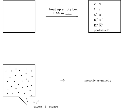
Figure 3: A Gedanken-Experiment that illustrates two of the three Sakharov conditions.

How the average baryon number is kept equal to zero in thermal equilibrium is a bit tricky, as the following example shows [2]. Consider an ensemble of a heavy particle species $X$ that has 2 baryon-number violating decay modes $X\to qq$ and $X\to\ell{\bar{q}}$ into quarks and leptons. (Take $q=d$ and $\ell=e$.) Further, assume that there is C and CP violation in these decays such that an asymmetry in the partial decay rates of $X$ and its antiparticle $\bar{X}$ is induced:

$$\Gamma(X\to qq)\>=\>(1+\epsilon)\Gamma_{0}\>,\qquad\Gamma({\bar{X}}\to{\bar{q}}{\bar{q}})\>=\>(1-\epsilon)\Gamma_{0}\>,$$ (29)

and there will also be an asymmetry for the other channel. CPT invariance is supposed to hold. Then the total decays rates of $X$ and $\bar{X}$ are equal. In the decays of $X,\bar{X}$ a non-zero baryon number $\Delta B$ is generated. The ensemble is supposed to be in thermal equilibrium. One might be inclined to appeal to the principle of detailed balance which would tell us that the inverse decay $qq\to X$ is more likely than ${\bar{q}}{\bar{q}}\to{\bar{X}}$, and the temporary excess $\Delta B\neq 0$ would be erased this way. However, this principle is based on $T$ invariance – but CPT invariance implies that this symmetry is broken because of CP violation. In fact applying a CPT transformation to the above decays, CPT invariance tells us that the inverse decays push $\Delta B$ into the same direction as (29):

$$\Gamma(qq\to X)\>=\>(1-\epsilon)\Gamma_{0}\>,\qquad\Gamma({\bar{q}}{\bar{q}}\to{\bar{X}})\>=\>(1+\epsilon)\Gamma_{0}\>.$$ (30)

The elimination of the baryon number $\Delta B$ is achieved by the B-violating reactions $qq\to\ell{\bar{q}}$, ${\bar{q}}{\bar{q}}\to{\bar{\ell}}q$, and the CPT-transformed reactions, where the $X,\bar{X}$ resonance contributions are to be taken out of the scattering amplitudes. It is the unitarity of the S matrix which does the job of keeping $<{\hat{B}}>_{T}=0$ in thermal equilibrium.

The following Gedanken-Experiment, sketched in Fig. 3, illustrates two of the three Sakharov conditions [16]. Let’s simulate the big bang by taking an empty box and heat it up to a temperature, say, above the nucleon mass. Pairs of particles and antiparticles are produced that start interacting with each other, instable particles decay, etc. The $K^{0}$ and ${\bar{K}}^{0}$ evolve in time as coherent superpositions of $K_{L}$ and $K_{S}$, and these states have CP-violating decays, for instance the observed non-leptonic modes $K_{L}\to\pi\pi$, and there is the observed CP-violating charge asymmetry in the semileptonic decays $K_{L}\to\pi^{\mp}\ell^{\pm}\nu$ [8]. When analyzing the semileptonic decays of ${K}^{0}$ and ${\bar{K}}^{0}$ one finds that slightly more $\pi^{-}\ell^{+}\nu_{\ell}$ are produced than $\pi^{+}\ell^{-}{\bar{\nu}}_{\ell}$ , by about one part in $10^{3}$. Hence, although initially there were equal numbers of $K^{0}$ and ${\bar{K}}^{0}$, their decays produce more $\pi^{-}$ than $\pi^{+}$. Yet as long as the system is in thermal equilibrium, CP violation in the reactions including $\pi^{+}\ell^{-}\leftrightarrow\pi^{+}\pi^{-}{\nu}_{\ell}$ and $\pi^{-}\ell^{+}\leftrightarrow\pi^{+}\pi^{-}{\bar{\nu}}_{\ell}$ will wash out the temporary excess of $\pi^{-}$. However, if a thermal instability is created by opening the box for a while, the excess $\ell^{+}$ from neutral kaon decay have a chance to escape. Then the inverse reactions involving $\ell^{+}$ are blocked to some degree, and a mesonic asymmetry $(N_{\pi^{-}}-N_{\pi^{+}})>0$ is generated. Of course, we haven’t yet produced the real thing, as no B-violating interactions came into play.

In general, the Sakharov conditions are sufficient but not necessary for generating a non-zero baryon number. Each of them can be circumvented in principle [2]. For instance, if $H$ is not CPT invariant, the argumentation of eq. (28) fails. However, such ideas have so far not led to a satisfactory explanation of (26). For the baryogenesis scenarios that will be discussed in sections 5,6 the Sakharov conditions are necessary ones.

4 CP and B Violation in the Standard Model

The standard model of particle physics combined with the SCM has, it seems, all the ingredients for generating a baryon asymmetry. First we recall the salient features of the SM at temperatures $T\simeq 0$ which apply to present-day physics. The observed particle spectrum tells us that the electroweak gauge symmetry $SU(2)_{L}\times U(1)_{Y}$, for which there is solid empirical evidence, cannot be a symmetry of the ground state. In the SM this spontaneous symmetry breaking is accomplished by a $SU(2)_{L}$ doublet of scalar fields $\Phi(x)$, the Higgs field, that is assumed to have a non-zero ground state expectation value $<0|\Phi|0>=246$ GeV (see below). This classical field selects a direction in the internal $SU(2)_{L}\times U(1)_{Y}$ space and hence breaks the electroweak symmetry, leaving intact the gauge symmetry of electromagnetism. The $W$ and $Z$ bosons, quarks, and leptons acquire their masses by coupling to this field (which may be viewed as a Lorentz-invariant ether).

C and CP are violated by the charged weak quark interactions

$${\cal L}_{cc}\>=\>-\frac{g_{w}}{\sqrt{2}}{\bar{U}}_{L}\gamma^{\mu}V_{KM}D_{L}W_{\mu}^{+}\>+\>h.c.\,.$$ (31)

Here $U_{L}=(u_{L},c_{L},t_{L})^{T},$ $D_{L}=(d_{L},s_{L},b_{L})^{T},$ denote the left-handed quark fields ($q_{L}=(1-\gamma_{5})q/2$), $W_{\mu}^{+}$ is the W boson field, $g_{w}$ is the weak gauge coupling, and $V_{KM}$ is the Cabibbo-Kobayashi-Maskawa mixing matrix. CP is violated if the KM phase angle $\delta_{KM}\neq 0,\pm\pi$. By this “mechanism” the CP effects observed so far in the $K$ and $B$ meson systems (cf., e.g., [17, 18, 19]) can be explained.

There is also baryon number violation in the SM, but this is a subtle, non-perturbative effect which is completely negligible for particle reactions in the laboratories at present-day collision energies, but very significant for the physics of the early universe. Let us outline how this effect arises. From experience we know that baryon and lepton number, which are conventionally assigned to quarks and leptons as given in the table, are good quantum numbers in particle reactions in the laboratory.

	$q$	$\bar{q}$	$\ell$	${\bar{\ell}}$
B	1/3	-1/3	0	0
L	0	0	1	-1

In the SM this is explained by the circumstance that the SM Lagrangian ${\cal L}_{SM}(x)$, with its strong-interaction (QCD) and electroweak parts, has a global $U(1)_{B}$ and $U(1)_{L}$ symmetry: ${\cal L}_{SM}$ is invariant under the following two sets of global phase transformations of the quark and lepton fields $q=u,...,t;$ $\ell=e,...,\nu_{\tau}$:

$$q(x) \to e^{i\omega/3}q(x)\;,\hskip 28.45274pt\ell(x)\to\ell(x)\>,$$ (32)

$$\ell(x) \to e^{i\lambda}\ell(x)\;,\hskip 39.83368ptq(x)\to q(x)\>.$$ (33)

Applying Noether’s theorem we obtain the associated symmetry currents $J^{B}_{\mu}$ and $J^{L}_{\mu}$, which are conserved at the Born level:

$$\partial^{\mu}J^{B}_{\mu}\>=\>\partial^{\mu}\sum_{q}\frac{1}{3}{\bar{q}}\gamma_{\mu}q\>=\>0\,,$$ (34)

$$\partial^{\mu}J^{L}_{\mu}\>=\>\partial^{\mu}\sum_{\ell}{\bar{\ell}}\gamma_{\mu}\ell\>=\>0\,.$$ (35)

(The currents are to be normal-ordered.) Thus the associated charge operators

$${\hat{B}}\>=\>\int d^{3}xJ^{B}_{0}(x)\,,$$ (36)

$${\hat{L}}\>=\>\int d^{3}xJ^{L}_{0}(x)\,$$ (37)

are time-independent. At the level of quantum fluctuations beyond the Born approximation these symmetries are, however, explicitly broken because eqs. (34), (35) no longer hold. This is seen as follows. Decompose the vector current

$${\bar{f}}\gamma_{\mu}f\>=\>{\bar{f}}_{L}\gamma_{\mu}f_{L}\>+\>{\bar{f}}_{R}\gamma_{\mu}f_{R}\,,$$ (38)

where $f=q,\ell$, into its left- and right-handed pieces. Because of the clash between gauge and chiral symmetry at the quantum level the gauge-invariant chiral currents are not conserved: in the quantum theory the current-divergencies suffer from the Adler-Bell-Jackiw anomaly [20, 21]. For a gauge theory based on a gauge group $G$, which is a simple Lie group of dimension $d_{G}$, the anomaly equations for the L- and R-chiral currents ${\bar{f}}_{L}\gamma_{\mu}f_{L}$ and ${\bar{f}}_{R}\gamma_{\mu}f_{R}$ read

$$\partial^{\mu}{\bar{f}}_{L}\gamma_{\mu}f_{L}\> = \>-c_{L}\frac{g^{2}}{32\pi^{2}}F^{a}_{\mu\nu}{\tilde{F}}^{a\mu\nu}\,,$$ (39)

$$\partial^{\mu}{\bar{f}}_{R}\gamma_{\mu}f_{R}\> = \>+c_{R}\frac{g^{2}}{32\pi^{2}}F^{a}_{\mu\nu}{\tilde{F}}^{a\mu\nu}\,,$$ (40)

where $F^{a\mu\nu}$ is the (non)abelian field strength tensor ($a=1,...,d_{G}$) and ${\tilde{F}}^{a\mu\nu}=\epsilon^{\mu\nu\alpha\beta}F^{a}_{\alpha\beta}/2$ is the dual tensor, $g$ denotes the gauge coupling, and the constants $c_{L},c_{R}$ depend on the representation which the $f_{L}$ and $f_{R}$ form. Let us apply (38) - (40) to the above baryon and lepton number currents of the SM where the gauge group is $SU(3)_{c}\times SU(2)_{L}\times U(1)_{Y}$. Because gluons couple to right-handed and left-handed quark currents with the same strength, we have $c_{L}^{QCD}=c_{R}^{QCD}$. Therefore $J^{B}_{\mu}$ has no QCD anomaly. However, the weak gauge bosons $W_{\mu}^{a},a=1,2,3,$ couple only to left-handed quarks and leptons, while the weak hypercharge boson couples to $f_{L}$ and $f_{R}$ with different strength. Hence $c^{W}_{R}=0$ and $c_{L}^{Y}\neq c_{R}^{Y}$. Putting everything together one obtains

$$\partial^{\mu}J^{B}_{\mu}\>=\>\partial^{\mu}J^{L}_{\mu}\>=\>\frac{n_{F}}{32\pi^{2}}(-g_{w}^{2}W^{a}_{\mu\nu}{\tilde{W}}^{a\mu\nu}+g^{\prime 2}B_{\mu\nu}{\tilde{B}}^{\mu\nu})\,,$$ (41)

where $W^{a}_{\mu\nu}$ and $B_{\mu\nu}$ denote the $SU(2)_{L}$ and $U(1)_{Y}$ field strength tensors, respectively, $g^{\prime}$ is the $U(1)_{Y}$ gauge coupling, and $n_{F}=3$ is the number of generations.

Eq. (41) implies that $\partial^{\mu}(J^{B}_{\mu}-J^{L}_{\mu})=0$. Thus the difference of the baryonic and leptonic charge operators ${\hat{B}}-{\hat{L}}$ remains time-independent also at the quantum level and therefore the quantum number

B - L is conserved in the SM.

How does B+L number violation come about? We note that the right hand side of eq. (41) can also be written as the divergence of a current $K^{\mu}$:

$$r.h.s.\;{\rm of}\;(\ref{eq:waekan})\>=\>n_{F}\partial_{\mu}K^{\mu}\,,$$ (42)

where

$$K^{\mu}\>=\;-\frac{g_{w}^{2}}{32\pi^{2}}2\epsilon^{\mu\nu\alpha\beta}W^{a}_{\nu}(\partial_{\alpha}W^{a}_{\beta}+\frac{g_{w}}{3}\epsilon^{abc}W^{b}_{\alpha}W^{c}_{\beta})+\frac{g^{\prime 2}}{32\pi^{2}}\epsilon^{\mu\nu\alpha\beta}B_{\nu}B_{\alpha\beta}\>.$$ (43)

Let’s integrate eq. (41), using (42), over space-time. Using Gauß’s law we convert these integrals into integrals over a surface at infinity. Let’s first do the surface integral for the right-hand side of (41). For hypercharge gauge fields $B_{\mu}$ with acceptable behaviour at infinity, that is, vanishing field strength $B_{\alpha\beta}$, the abelian part of $K_{\mu}$ makes no contribution to this integral. For the non-abelian gauge fields $W^{a}_{\nu}$ vanishing field strength implies that $2\epsilon_{\mu\nu\alpha\beta}\partial^{\alpha}W^{a\beta}=-g_{w}\epsilon_{\mu\nu\alpha\beta}\epsilon^{abc}W^{b\alpha}W^{c\beta}$ at infinity. Using this we obtain

$$\int d^{4}x\,\partial^{\mu}K_{\mu}\>=\;\frac{g_{w}^{3}}{96\pi^{2}}\int_{\partial V_{4}}dn^{\mu}\,\epsilon_{\mu\nu\alpha\beta}\epsilon^{abc}W^{a\nu}W^{b\alpha}W^{c\beta}\>.$$ (44)

Now we choose the surface $\partial V_{4}$ to be a large cylinder with top and bottom surfaces at $t_{f}$ and $t_{i}$, respectively, and let the volume of the cylinder tend to infinity. Because $\partial_{\mu}K^{\mu}$ is gauge-invariant, we may choose a special gauge. Choose the temporal gauge condition, $W^{a}_{0}=0$. Then there is no contribution from the integral over the coat of the cylinder and we obtain

$$\int d^{3}xdt\,\partial_{\mu}K^{\mu}\>=\;N_{CS}(t_{f})-N_{CS}(t_{i})\equiv\Delta N_{CS}\,,$$ (45)

where

$$N_{CS}(t)\>=\>\frac{g_{w}^{3}}{96\pi^{2}}\int d^{3}x\,\epsilon_{ijk}\epsilon^{abc}W^{ai}W^{bj}W^{ck}$$ (46)

is the Chern-Simons number. This integral assigns a topological “charge” to a classical gauge field. Actually $N_{CS}$ is not gauge invariant but $\Delta N_{CS}$ is. A nonabelian gauge theory like weak-interaction $SU(2)_{L}$ is topologically non-trivial, which is reflected by the fact that it has an infinite number of ground states whose vacuum gauge field configurations have different topological charges $\Delta N_{CS}=0,\pm 1,\pm 2,\ldots$ Imagine the set of gauge and Higgs fields and consider the energy functional $E[field]$ that forms a hypersurface over this infinite-dimensional space. The ground states with different topological charge are separated by a potential barrier. In Fig. 4 a one-dimensional slice through this hypersurface is drawn. The direction in field space has been chosen such that the classical path from one ground state to another goes over a pass of minimal height.

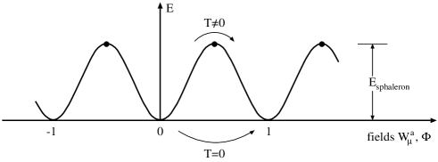
Figure 4: The periodic vacuum structure of the standard electroweak theory. The direction in field space has been chosen as described in the text. The schematic diagram shows the energy of static gauge and Highs field configurations $W^{a}_{\mu}({\bf x}),\Phi({\bf x})$. The integers are the Chern-Simons number $N_{CS}$ of the respective zero-energy field configuration.

Finally we perform the integral over the left-hand sides of (41) and get the result

$$\Delta{\hat{B}}\>=\>\Delta{\hat{L}}\>=\>n_{F}\Delta N_{CS}\,,$$ (47)

with $\Delta{\hat{Q}}\equiv{\hat{Q}}(t_{f})-{\hat{Q}}(t_{i}),$ $Q=B,L$. Eq. (47) is to be interpreted as follows. As long as we consider small gauge field quantum fluctuations around the perturbative vacuum configuration $W^{a}_{\mu}=0$ the right-hand side of (47) is zero, and $B$ and $L$ number remain conserved. This is the case in perturbation theory to arbitrary order where B- and L-violating processes have zero amplitudes. However, large gauge fields $W^{a}_{\mu}\sim 1/g_{w}$ with nonzero topological charge $\Delta N_{CS}=\pm 1,\pm 2,...$ exist. As discovered by ‘t Hooft [22] they can induce transitions at the quantum level between fermionic states $|i,t_{i}>$ and $|f,t_{f}>$ with baryon and lepton numbers that differ according to the rule (47):

$$\Delta{B}\>=\>\Delta{L}\>=\>n_{F}\Delta N_{CS}\,.$$ (48)

This selection rule tells us that $B$ and $L$ must change by at least 3 units. A closer inspection of the global $U(1)$ symmetries and associated currents shows that, in situations where fermion masses can be neglected, the selection rule can be refined: there is a change in quantum numbers by the same amount for every generation. Thus, e.g., $\Delta{L_{e}}=\Delta{L_{\mu}}=\Delta{L_{\tau}}=\Delta{B}/3=\Delta N_{CS}$.

The dominant B- and L-violating transitions are between states $|i,t_{i}>$ and $|f,t_{f}>$ where $|\Delta{B}|=|\Delta{L}|$ changes by 3 units. At temperature $T=0$, transitions with $|\Delta{B}|=|\Delta{L}|=3$ are induced by the (anti)instanton [23], a gauge field which connects two vacuum configurations whose topological charge differ by $\pm 1$. When put into the temporal gauge $W^{a}_{0}=0$ then the instanton field $W^{a}_{i}({\bf x},t)$ approaches, for instance, $W^{a}_{i}=0$ at $t_{i}\to-\infty$ and a topologically non-trivial vacuum configuration with $N_{CS}=1$ at $t_{f}\to+\infty$, as indicated in Fig. 4. The corresponding amplitudes $<f,t_{f}|i,t_{i}>$ involve 9 left-handed quarks (right-handed $\bar{q}$) – where each generation participates with 3 different color states – and 3 left-handed leptons (right-handed $\bar{\ell}$), one of each generation. One of the possible amplitudes is depicted in Fig. 5. Hence we have, for instance, the anti-instanton induced reaction with $\Delta{B}=\Delta{L}=-3$:

$$u+d\to{\bar{d}}+2{\bar{s}}+{\bar{c}}+2{\bar{b}}+{\bar{t}}+{\bar{\nu}_{e}}+{\bar{\nu}_{\mu}}+{\bar{\nu}_{\tau}}\,.$$ (49)

Figure 5: An example of a (B+L)-violating standard model amplitude. The arrows indicate the flow of the fermionic quantum numbers.

What is the probability for such a transition to occur? It is clear from Fig. 4 that it corresponds to a tunneling process. Thus it must be exponentially suppressed. The classic computation of ‘t Hooft [22, 24] implies, for energies $E_{c.m.}(ud)\lesssim{\cal O}(1\,TeV)$, a cross-section

$$\sigma_{B\!\!\!/+L\!\!\!/}\>\propto\>e^{-4\pi/\alpha_{w}}\>\sim\>10^{-164}\,,$$ (50)

where $\alpha_{w}=g_{w}^{2}/4\pi\simeq 1/30$.

When the standard model is coupled to a heat bath of temperature $T$, the situation changes. As was first shown in [25] (see also [26]), at very high temperatures $T\gtrsim T_{EW}\sim 100$ GeV the B- and L-violating processes in the SM are fast enough to play a significant role in baryogenesis. In order to understand this we have again a look at Fig. 4. The ground states with different $N_{CS}$ are separated by a potential barrier of minimal height

$$E_{sph}(T)\>=\>\frac{4\pi}{g_{w}}v_{T}f(\frac{\lambda}{g_{w}})\>,$$ (51)

where $v_{T}\equiv<0|\Phi|0>_{T}$ is the vacuum expectation value (VEV) of the SM Higgs doublet field $\Phi(x)$ at temperature T. At $T=0$ we have $v_{T=0}=246$ GeV. The parameter $f$ varies between $1.6<f<2.7$ depending on the value of the Higgs self-coupling $\lambda$, i.e., on the value of the SM Higgs mass. This yields $E_{sph}(T=0)\simeq 8-13$ TeV. The subscript “sph” refers to the sphaleron, a gauge and Higgs field configuration of Chern-Simons number 1/2 (+ integer) which is an (unstable) solution of the classical field equations of the SM gauge-Higgs sector [27, 28]. These kind of field configurations (their locations are indicated by the dots in Fig. 4) lie on the respective minimum energy path from one ground state to another with different Chern-Simons number. Fig. 4 suggests that the rate of fermion-number non-conserving transitions will be proportional to the Boltzmann factor $\exp(-E_{sph}(T)/T)$ as long as the energy of the thermal excitations is smaller than that of the barrier, while unsuppressed transitions will occur above that barrier.

At this point we recall that the electroweak (EW) $SU(2)_{L}\times U(1)_{Y}$ gauge symmetry was unbroken at high temperatures, that is, in the early universe. The critical temperature $T_{EW}$ where – running backwards in time – the transition from the broken phase with Higgs VEV $v_{T}\neq 0$ to the symmetric phase with $v_{T}=0$ occurs is, in the SM, about 100 GeV. (A discussion of this transition will be given in the next section.) Hence the B- and L-violating transition rates of the SM will no longer be exponentially suppressed above this temperature. Detailed investigations have led to the following results:
$\bullet$ In the phase where the EW gauge is broken, i.e., $T<T_{EW}\sim 100$ GeV, the sphaleron-induced ${B\!\!\!/+L\!\!\!/}$ transition rate per volume $V$ is given by (see, e.g., [4, 29])

$$\frac{\Gamma^{sph}_{B\!\!\!/+L\!\!\!/}}{V}=\kappa_{1}\left(\frac{m_{W}}{\alpha_{w}T}\right)^{3}m_{W}^{4}\exp(-E_{sph}(T)/T)\,,$$ (52)

where $m_{W}(T)=g_{w}v_{T}/2$ is the temperature-dependent mass of the W boson and $\kappa_{1}$ is a dimensionless constant.
$\bullet$ The calculation of the transition rate in the unbroken phase is very difficult. On dimensional grounds we expect this rate per volume to be proportional to $T^{4}$. Recent investigations [30, 31] yield for $T>T_{EW}\sim 100$ GeV:

$$\frac{\Gamma^{sph}_{B\!\!\!/+L\!\!\!/}}{V}=\kappa_{2}\,\alpha_{w}^{5}T^{4}\,,$$ (53)

with $\kappa_{2}\sim 21$.

By comparing $\Gamma^{sph}_{B\!\!\!/+L\!\!\!/}$ above $T_{EW}$ with the expansion rate $H$ given in (23), we can assess whether the (B+L)-violating SM reactions, which conserve B-L, are fast enough to keep up with the expansion of the early universe in the radiation dominated epoch. From the requirement $\Gamma^{sph}_{B\!\!\!/+L\!\!\!/}>>H$ one obtains that these processes are in thermal equilibrium for temperatures

$$T_{EW}\;\sim\;100\>{\rm GeV}\;<\;T\;\;\lesssim\;10^{12}\>{\rm GeV}\>.$$ (54)

This result provides an important constraint on any baryogenesis mechanism which operates above $T_{EW}$. If the B- and L-violating interactions involved in this mechanism conserve B-L, then any excess of baryon and lepton number generated above $T_{EW}$ will be washed out by the B- and L-nonconserving SM sphaleron-induced reactions. Hence baryogenesis scenarios above $T_{EW}$ must be based on particle physics models that violate also B-L. Examples will be discussed in section 6.

5 Electroweak Baryogenesis

We haven’t discussed yet which phenomenon could possibly provide the third Sakharov ingredient, the departure from thermal equilibrium, if one attempts to explain the baryon asymmetry within the SM of particle physics. A little thought reveals that a baryogenesis scenario based on the SM requires that the thermal instability must come from the electroweak phase transition. First of all, the expansion rate of the universe at temperatures, say, $T\lesssim 10^{12}$ GeV is too slow for causing a departure from local thermal equilibrium: the reaction rates of most of the SM particles, which are typically of the order of $\Gamma\sim\alpha_{w}^{2}T$ or larger, are much larger than the expansion rate (23), even for extremely high temperatures. Further, the SM charged weak quark current interactions lead to CP-violating effects only because, apart from a non-trivial KM phase, the u- and d-type quarks have non-degenerate masses (see eq. (95) below). These masses are generated at the EW transition, while all SM particles are massless above $T_{EW}$. If $\Delta B\neq 0$ was created at the EW transition it would be – if the phase change was strongly first order – frozen in during the later evolution of the universe, as the B- and L-violating reactions below $T_{EW}$ would be strongly suppressed (see eq. (52) and below). However, the investigations of refs. [34, 35, 36] have shown that the EW transition in the SM fails to provide the required thermal instability.

Before reviewing the results on the nature of the EW transition in the SM let us recall some basic concepts about phase transitions. Consider Fig. 6 where the pressure versus temperature phase diagram of water is sketched. We concentrate on the vapor $\leftrightarrow$ liquid transition. The curve to the right of the triple point is the so-called vapor-pressure curve. For values of $p,T$ along this line there is a coexistence of the liquid and gaseous phases. A change of the parameters across this curve leads to a first order phase transition which becomes weaker along the curve. The endpoint corresponds to a second order transition. Beyond that point there is a smooth cross-over from the gaseous to the liquid phase and vice versa.

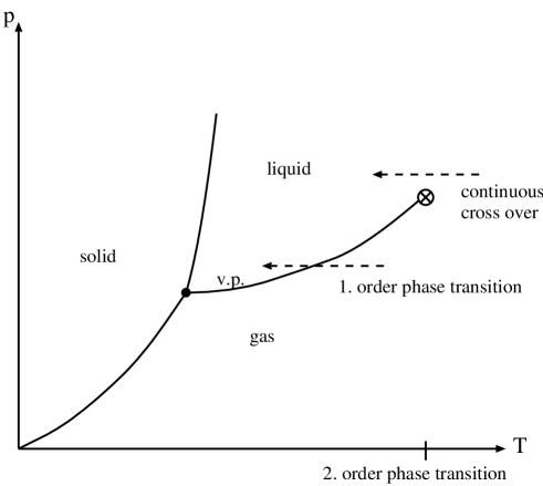
Figure 6: The phase diagram of water.

The nature of a phase transition can be characterized by an order parameter appropriate to the system. For the vapor-liquid transition the order parameter is the difference in the densities of water in the liquid and gaseous phase, ${\tilde{\rho}}=\rho_{liquid}-\rho_{vapour}$. In the case of a strong first order phase transition the order parameter has a strong discontinuity at the critical temperature $T_{c}$ where the transition occurs: in the example at hand ${\tilde{\rho}}$ is very small in the vapor phase but it makes a sizeable jump at $T_{c}$ because of the coexistence of both phases – see Fig. 7. That’s what we need in a successful EW baryogenesis scenario! In case of a second order phase transition the order parameter changes also rapidly in the vicinity of $T_{c}$, but the change is continuous. In the cross-over region of the phase diagram the continuous change of ${\tilde{\rho}}$ as a function of $T$ is less pronounced.

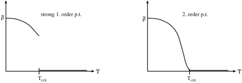
Figure 7: The behaviour of the order parameter ${\tilde{\rho}}$ in the case of a strong first order and a second order transition.

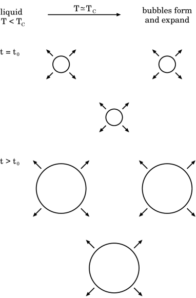
Figure 8: Dynamics of a first-order liquid-vapor phase transition: Formation and expansion of vapor bubbles.

So far to the statics of phase transitions. As to their dynamics, we know from experience how the first-order liquid-vapor transition evolves in time. Heating up water, vapor bubbles start to nucleate slightly below $T=T_{c}$ within the liquid. They expand and finally percolate above $T_{c}$. This is illustrated in Fig 8. Drawing the analogy to the early universe we should, of course, rather consider the cooling of vapor and its transition to a liquid through the formation of droplets.

A standard theoretical method to determine the nature of a phase transition in a classical system, like the vapor$\leftrightarrow$liquid or paramagnetic$\leftrightarrow$ferromagnetic transition is as follows. Let ${\cal H}={\cal H}(s)$ be the classical Hamiltonian of the system, where $s({\bf x})$ is a (multi-component) classical field. In the case of water $s({\bf x})$ is the local density, while for a magnetic material $\vec{s}({\bf x})$ denotes the three-component local magnetization. From the computation of the partition function $Z$ we obtain the Helmholtz free energy $F=-T\ln Z$ from which the thermodynamic functions of interest can be derived. In particular we can compute the order parameter $s_{av}=<\sum_{\bf x}s({\bf x})>_{T}$ and study its behaviour as a function of temperature.

The investigation of the static thermodynamic properties of gauge field theories proceeds along the same lines. In the case of the standard electroweak theory the role of the order parameter is played by the VEV of the $SU(2)_{L}$ Higgs doublet field $\Phi$. This becomes obvious when we recall the following. Experiments tell us that the $SU(2)_{L}\times U(1)_{Y}$ gauge symmetry is broken at $T=0.$ For the SM this means that the mass parameter in the Higgs potential must be tuned such that there is a non-zero Higgs VEV. On the other hand it was shown a long time ago [32] that at temperatures significantly larger than, say, the W boson mass the Higgs VEV is zero and the $SU(2)_{L}\times U(1)_{Y}$ gauge symmetry is restored. (This will be shown below.) Hence during the evolution of the early universe the Higgs field must have condensed at some $T=T_{c}$. The order of this phase transition is deduced from the behaviour of the Higgs VEV (and other thermodynamic quantities) around $T_{c}$.

Let’s couple the standard electroweak theory to a heat bath of temperature $T$. The free energy $F=-T\ln Z$ is obtained from the Euclidean functional integral

$$F(J,T)\>=\>-T\ln{\left[\int_{\beta}{\cal D}[{\rm fields}]\exp(-\int_{\beta}dx({\cal L}_{EW}+J\cdot\Phi))\right]}\>,$$ (55)

where ${\cal L}_{EW}={\cal L}_{EW}(\Phi,W_{\mu}^{a},B_{\mu},q,\ell)$ denotes the Euclidian version of the electroweak SM Lagrangian, $J$ is an auxiliary external field, $\beta=1/T$,

$$\int_{\beta}dx=\int^{\beta}_{0}d\tau\int_{V}d^{3}x\>,$$ (56)

and the subscript $\beta$ on the functional integral indicates that the bosonic (fermionic) fields satisfy (anti)periodic boundary conditions at $\tau=0$ and $\tau=\beta$. From the free energy density $F(J,T)/V$ the effective potential $V_{eff}(\phi,T)$ is obtained by a Legendre transformation, where $\phi=\partial F/\partial J|_{J=0}$ is the expectation value of the Higgs doublet field, $\phi=<\Phi>_{T}$. (Actually in order to compare with numerical lattice calculations it is useful to employ a gauge-invariant order parameter.) Recall that the effective potential $V_{eff}(\phi,T)$ is the energy density of the system in that state $|a>_{T}$ in which the expectation value $<a|\Phi|a>_{T}$ takes the value $\phi$. Hence by computing the stationary point(s), $\partial V_{eff}(\phi,T)/\partial\phi=0$, the ground-state expectation value(s) $\phi$=$<0|\Phi|0>_{T}$ of $\Phi$ at a given temperature $T$ are determined. If at some $T=T_{c}$ two minima are found then this signals two coexisting phases and a first order phase transition.

5.1 Why the SM fails

Let us now discuss the effective potential of the SM. At $T=0$ the tree-level effective potential is just the classical Higgs potential $V_{tree}=-\mu^{2}(\Phi^{\dagger}\Phi)+\lambda(\Phi^{\dagger}\Phi)^{2}$. Choosing the unitary gauge, $\Phi^{unitary}=(0,\phi/\sqrt{2})$ with $\phi\geq 0$ we have

$$V_{tree}(\phi)\>=\>-\frac{\mu^{2}}{2}\phi^{2}+\frac{\lambda}{4}\phi^{4}\>,$$ (57)

where $\lambda>0$ and, by assumption, $\mu^{2}>0$ in order that the Higgs field is non-zero in the state of minimal energy: $\phi_{0}\equiv<0|\Phi|0>_{T=0}\equiv v_{T=0}/\sqrt{2}=\sqrt{\mu^{2}/\lambda}$, and $v_{T=0}$ is fixed by, e.g., the experimental value of the W boson mass to $v_{T=0}=246$ GeV. The mass of the SM Higgs boson is given by

$$m_{H}\>=v_{T=0}\sqrt{2\lambda}+{\rm quantum}\;{\rm corrections}\>.$$ (58)

The experiments at LEP2 have established the lower bound $m_{H}>114$ GeV [33]. Hence the SM Higgs self-coupling $\lambda>0.33$.

At $T\neq 0$ the SM effective potential is computed at the quantum level as outlined above. Because the gauge coupling $g^{\prime}$ and the Yukawa couplings of quarks and leptons $f\neq t$ ($t$ denotes the top quark) to the Higgs doublet $\Phi$ are small, the contributions of the hypercharge gauge boson and of $f\neq t$ may be neglected. This is usually done in the literature. Let us first discuss, for illustration, the effective potential computed to one-loop approximation for the now obsolete case of a very light Higgs boson. For high temperatures $V_{eff}$ is given by

$$V_{eff}(\phi,T)\>=\frac{1}{2}a(T^{2}-T_{1}^{2})\phi^{2}-\frac{1}{3}bT\phi^{3}+\frac{1}{4}\lambda\phi^{4}\>,$$ (59)

where

$$a\>=\>\frac{3}{16}g_{w}^{2}+(\frac{1}{2}+\frac{m_{t}^{2}}{m_{H}^{2}})\lambda\;,\;b\>=\>9\frac{g_{w}^{3}}{32\pi}\;,\;T_{1}\>=\;\frac{m_{H}}{2\sqrt{a}}\;,$$ (60)

and $m_{t}$ is the mass of the top quark. The term cubic in $\phi$ is due to fluctuations at $T\neq 0$. If the Higgs boson was light the quartic term would be small. Inspecting eq. (59) we recover the result quoted above that at high temperatures the Higgs field is zero in the ground state. When the temperature is lowered we find that at $T_{c}=T_{1}/\sqrt{1-2b^{2}/(9a\lambda)}>T_{1}$ a first order phase transition occurs: the effective potential $V_{eff}$ has two energetically degenerate minima: one at $\phi=0$ and the other at

$$v_{T_{c}}\>\equiv\>\phi_{crit}\>=\>\frac{2b}{3\lambda}T_{c}\>,$$ (61)

separated by an energy barrier, see Fig. 9. At $T_{c}$ the free energy of the symmetric and of the broken phase are equal; however, the universe remains for a while in the symmetric phase because of the energy barrier. As the universe expands and cools down further, bubbles filled with the Higgs condensate start to nucleate at some temperature below $T_{c}$. These bubbles become larger by releasing latent heat, percolate, and eventually fill the whole volume at $T=T_{1}$. Bubble nucleation and expansion are non-equilibrium phenomena which are difficult to compute.

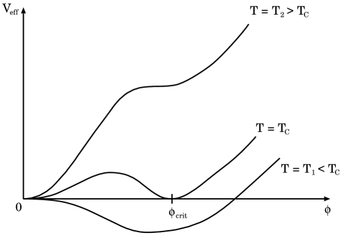
Figure 9: Behaviour of $V_{eff}$ in the case of a first order phase transition.

Fig. 10 shows the behaviour of $V_{eff}(\phi,T)$ in the case of a second order phase transition. In this case there are no energetically degenerate minima separated by a barrier at $T=T_{c}$, i.e., no bubble nucleation and expansion. The Higgs field gradually condenses uniformly at $T\lesssim T_{c}$ and grows to its present value as the system cools off.

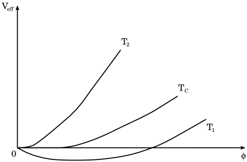
Figure 10: Behaviour of $V_{eff}$ in the case of a second order phase transition.

The value of the critical temperature depends on the parameters of the respective model and is obtained by detailed computations (see the references given below). Nevertheless, we may use the above formula for $T_{c}$ for a crude estimate and obtain $T_{c}\sim$ 70 GeV for $m_{H}=100$ GeV. (For a more precise value, see below.) With eqs. (5) and (23) we then estimate that the EW phase transition took place at a time $t_{EW}\sim 5\times 10^{-11}$ s after the big bang. This implies that the causal domain, the diameter of which is given by $d_{H}(t)=2t$ in the radiation-dominated era, was then of the order of a few centimeters.

Back to baryogenesis. It should be clear now why a strong first order EW phase transition is required. In this case the time scale associated with the nucleation and expansion of Higgs bubbles is comparable with the time scales of the particle reactions. This causes a departure from thermal equilibrium. How is this to be quantified? Let’s consider one of the bubbles with $v_{T}\neq 0$ which, after expansion and percolation, eventually become our world. The bubble must get filled with more quarks than antiquarks such that $n_{B}/s\sim 10^{10}$ and this ratio remains conserved. This means that baryogenesis has to take place outside of the bubble while the sphaleron-induced (B+L)-violating reactions must be strongly suppressed within the bubble. In order that the sphaleron rate, which in the broken phase is given by eq. (52), $\Gamma^{sph}_{B\!\!\!/+L\!\!\!/}\propto\exp{(-4\pi fv_{T}/g_{w}T)}$, is practically switched off, the order parameter must jump at $T_{c}$, from $\phi=0$ in the symmetric phase to a value $v_{T_{c}}$ in the broken phase such that

$$\frac{v_{T_{c}}}{T_{c}}\>\gtrsim\>1\>.$$ (62)

This is the condition for a first order transition to be strong.

In view of the experimental lower bound $m_{H}^{SM}>114$ GeV, the formulae (59), (60) for $V_{eff}$ which are valid only for a very light Higgs boson no longer apply. Nevertheless, eq. (61) shows that the discontinuity gets weaker when the Higgs mass is increased. The strength of the electroweak phase transition has been studied for the SM $SU(2)$ gauge-Higgs model as a function of the Higgs boson mass with analytical methods [34], and numerically with 4-dimensional [35] and 3-dimensional [36] lattice methods. These results quantify the qualitative features discussed above: the strength of the phase transition changes from strongly first order ($m_{H}\lesssim$ 40 GeV) to weakly first order as the Higgs mass is increased, ending at $m_{H}\simeq$ 73 GeV [37, 38, 39] where the phase transition is second order (cf. the liquid-vapor transition discussed above). The corresponding critical temperature is $T_{c}\simeq$ 110 GeV [40]. For larger values of $m_{H}$ there is a smooth cross-over between the symmetric and the broken phase.

Thus the result of the LEP2 experiments, $m^{SM}_{H}>$114 GeV, leads to the following conclusion: if the SM Higgs mechanism provides the correct description of electroweak symmetry breaking then the EW phase transition in the early universe does not provide the thermal instability required for baryogenesis. The B-violating sphaleron processes are only adiabatically switched off during the transition from $T>T_{c}$ to $T<T_{c}$; they are still thermal for $T\lesssim T_{c}$. Thus the standard model of particle physics cannot explain the BAU $\eta$ – irrespective of the role that SM CP violation may play in this game.

5.2 EW Phase Transition in SM Extensions

Of course, whether or not the SM Higgs field or some other mechanism provides the correct description of EW symmetry breaking remains to be clarified. In fact, this is the most important unsolved problem of present-day particle physics. Future collider experiments hope to resolve this issue. On the theoretical side, a number of extensions and alternatives to the SM Higgs mechanism have been discussed for quite some time. One may distinguish between models which postulate elementary Higgs fields (i.e., the associated spin-zero particles have pointlike couplings up to some high energy scale $E\gg 100$ GeV) which trigger the breakdown of $SU(2)_{L}\times U(1)_{Y}$, and others which assume that it is caused by the Bose condensation of (new) heavy fermion-antifermion pairs. The dynamics of the symmetry breaking sector of these models can change the order of the EW phase transition, as compared with the SM. Let’s briefly discuss results for some models that belong to the first class. The presently most popular extensions of the SM are supersymmetric (SUSY) extensions, in particular the minimal supersymmetric standard model (MSSM), the Higgs sector of which contains two Higgs doublets. Although the requirement of SUSY breaking to be soft does not allow for independent quartic couplings in the Higgs potential $V(\Phi_{1},\Phi_{2})$, the number of parameters of the scalar sector of this model is larger than that of the SM and a first order transition can be arranged. Investigations of $V_{eff}$ at $T\neq 0$ show that there is a region in the MSSM parameter space which allows for a sufficiently strong first order EW phase transition (see, for instance, the reviews [40, 41] and references therein). The condition for this is that the mass of the scalar partner $\tilde{t}_{R}$ of the right-handed top quark $t_{R}$ must be sufficiently light and the mass of $\tilde{t}_{L}$ must be sufficiently heavy. An upper bound on the mass of the lightest neutral Higgs boson $H_{1}$ of the model obtains from the requirement that the mass of $\tilde{t}_{L}$ should not be unnaturally large. In summary, the MSSM predicts a sufficiently strong 1st order EW phase transition if

$$m_{H_{1}}\>\lesssim\>105\>-\>115\>{\rm GeV}\,,\hskip 28.45274ptm_{\tilde{t}_{R}}\>\lesssim\>170\>{\rm GeV}\,\>.$$ (63)

In the next-to-minimal SUSY model which contains an additional gauge singlet Higgs field a strong first order transition can be arranged quite easily [68].

Non-supersymmetric SM extensions may be, in general, less motivated than SUSY models, but several of these models are, nevertheless, worth to be studied as they predict interesting phenomena. For illustrative purposes we mention here only the class of 2 Higgs doublet models (2HDM) where the field content of the SM is extended by an additional Higgs doublet, leading to a physical particle spectrum which includes 3 neutral and one charged Higgs particle. The general, renormalizable and $SU(2)_{L}\times U(1)_{Y}$ invariant Higgs potential $V(\Phi_{1},\Phi_{2})$ contains a large number of unknown parameters. Therefore, it is not surprising that in these models, too, the requirement of a strong 1st order EW transition can be arranged quite easily as studies of the finite-temperature effective potential show (see, for instance, [44]). No tight upper bound on the mass of the lightest Higgs boson obtains.

5.3 CP Violation in SM Extensions

Another aspect of SM extensions, namely non-standard CP violation, is also essential for baryogenesis scenarios. SM extensions as those mentioned above involve, in particular, an extended non-gauge sector; that is to say, a richer set of Yukawa and Higgs-boson self-interactions than in the SM. It is these interactions that break, in general, CP invariance. Thus, in SM extensions additional sources of CP violation besides the KM phase are usually present. We shall confine ourselves to 2 examples. (For a review, see for instance [45].)

5.3.1 Higgs sector CPV

An interesting possibility is CP violation (CPV) by an extended Higgs sector which can occur already in the 2-Higgs doublet extensions of the SM. Consider the class of 2HDM which are constructed such that flavour-changing neutral (pseudo)scalar currents are absent at tree level. The appropriate $SU(2)_{L}\times U(1)_{Y}$ invariant tree-level Higgs potential $V(\Phi_{1},\Phi_{2})$ of these models may be represented in the following way:

$$V_{tree}(\Phi_{1},\Phi_{2})\> = \>\lambda_{1}(2\Phi_{1}^{\dagger}\Phi_{1}-v_{1}^{2})^{2}+\lambda_{2}(2\Phi^{\dagger}_{2}\Phi_{2}-v_{2}^{2})^{2}$$ (64)

$$+\,\lambda_{3}[(2\Phi^{\dagger}_{1}\Phi_{1}-v_{1}^{2})+(2\Phi^{\dagger}_{2}\Phi_{2}-v_{2}^{2})]$$

$$+\,\lambda_{4}[(\Phi_{1}^{\dagger}\Phi_{1})(\Phi_{2}^{\dagger}\Phi_{2})-(\Phi_{1}^{\dagger}\Phi_{2})(\Phi_{2}^{\dagger}\Phi_{1})]$$

$$+\,\lambda_{5}[2{\rm Re}(\Phi_{1}^{\dagger}\Phi_{2})-v_{1}v_{2}\cos\xi]^{2}$$

$$+\,\lambda_{6}[2{\rm Im}(\Phi_{1}^{\dagger}\Phi_{2})-v_{1}v_{2}\sin\xi]^{2}\>,$$

where $\lambda_{i},v_{1},v_{2}$ and $\xi$ are real parameters and the parameterization of $V_{tree}$ is chosen such that the Higgs fields have non-zero VEVs in the state of minimal energy.

Performing a CP transformation,

$$\Phi_{1,2}(\mbox{\bf x},t)\quad\stackrel{{\scriptstyle CP}}{{\longrightarrow}}\quad e^{i\alpha_{1,2}}\,\Phi_{1,2}^{\dagger}(-\mbox{\bf x},t)\>,$$ (65)

we see that $H_{V}=\int d^{3}x\,V_{tree}(\Phi_{1},\Phi_{2})$ is CP-noninvariant if $\xi\neq 0$. Notice that it is unnatural to assume $\xi=0$. Even if this was so at tree level, the non-zero KM phase $\delta_{KM}$, which is needed to explain the observed CPV in $K$ and $B$ meson decays, would induce a non-zero $\xi$ through radiative corrections.

From eq. (64) we read off that at zero temperature the neutral components of the Higgs doublet fields have, in the electric charge conserving ground state, the expectation values

$$<0|\phi^{0}_{1}|0>\>=\>v_{1}e^{\xi_{1}}/\sqrt{2}\,,\qquad<0|\phi^{0}_{2}|0>\>=\>v_{2}e^{i\xi_{2}}/\sqrt{2}\,,$$ (66)

where $v=\sqrt{v_{1}^{2}+v_{2}^{2}}=246$ GeV, and $\xi_{2}-\xi_{1}=\xi$ is the physical CPV phase.

The spectrum of physical Higgs boson states of the two-doublet models consists of a charged Higgs boson and its antiparticle, $H^{\pm}$, and three neutral states. As far as CPV is concerned, $H^{\pm}$ carries the KM phase. This particle affects the (CPV) phenomenology of flavor-changing $|\Delta F|=2$ neutral meson mixing and $|\Delta F|=1$ weak decays of mesons and baryons. ( Experimental data on $b\to s+\gamma$ imply that this particle must be quite heavy, $m_{H^{+}}>$ 210 GeV.)

Let’s briefly discuss some implications of Higgs sector CPV for present-day physics. If $\xi$ were zero, the set of neutral Higgs boson states would consist of two scalar (CP=1) and one pseudoscalar (CP= –1) state. If $\xi\neq 0$ these states mix. As a consequence the 3 mass eigenstates, $|\varphi_{1,2,3}>$, no longer have a definite CP parity. That is, they couple both to scalar and to pseudoscalar quark and lepton currents. In terms of Weyl fields the corresponding Lagrangian reads

$${\cal L}_{\varphi}=-\sum_{\psi}c_{\psi}\frac{m_{\psi}}{v}{\bar{\psi}_{L}}\psi_{R}\varphi\>+\>h.c.\>.$$ (67)

The sum over the Higgs fields $i=1,2,3$ is implicit, $\psi$ denotes a quark or lepton field, $m_{\psi}$ is the mass of the associated particle, and the dimensionless reduced Yukawa couplings $c_{\psi}=a_{\psi}+ib_{\psi}$ ($a_{\psi},b_{\psi}$ real) depend on the parameters of the Higgs potential and on the type of model.

The Yukawa interaction (67) leads to CPV in $flavour$-$diagonal$ reactions for quarks and for leptons $\psi$. The induced CP effects are proportional to some power $(m_{\psi})^{p}$. For example, consider the reaction $\psi{\bar{\psi}}\to\psi{\bar{\psi}}$. The exchange of a $\varphi$ boson at tree level induces an effective CPV interaction of the form $({\bar{\psi}}\psi)({\bar{\psi}}i\gamma_{5}\psi)$ with a coupling strength proportional to $m_{\psi}^{2}/m^{2}_{\varphi}$. The search for non-zero electric dipole moments (EDM) of the electron and the neutron has traditionally been a sensitive experimental method to trace non-SM CP violation [46]. If a light $\varphi$ boson exists ($m_{\varphi}\sim 100$ GeV) and the CPV phase $\xi$ is of order 1 the Yukawa interaction (67) can induce electron and neutron EDMs of the same order of magnitude as their present experimental upper bounds.

What happens at the EW phase transition in the early universe? We assume that the parameters of the 2HDM are such that the transition is strongly first order. Moreover, in order to simplify the discussion we assume that the passage from the symmetric to the broken phase occurs in one step, at some temperature $T_{c}$. Somewhat below $T_{c}$ bubbles filled with Higgs fields start to nucleate and expand. That is, the Higgs VEVs are space and time dependent. Let’s consider, for simplicity, only one of the bubbles and assume its expansion to be spherically symmetric. When the bubble has grown to some finite size we can use the following one-dimensional description. Consider the rest frame of the bubble wall. The wall is taken to be planar and the expansion of the bubble is taken along the $z$ axis. The wall, i.e., the phase boundary has some finite thickness $l_{wall}$, extending from $z=0$ to $z=z_{0}$. The symmetric phase lies to the right of this boundary, $z>z_{0}$ while the broken phase lies to the left, $z<0$. Thus the neutral Higgs fields have VEVs whose magnitudes and phases vary with $z$:

$$<0|\phi^{0}_{1}|0>_{T}\>=\>\frac{\rho_{1}(z)}{\sqrt{2}}e^{i\theta(z)}\,,\qquad<0|\phi^{0}_{2}|0>_{T}\>=\>\frac{\rho_{2}(z)}{\sqrt{2}}e^{i\omega(z)}\,.$$ (68)

In the symmetric phase, $z\gg z_{0}$, both VEVs vanish, whereas in the broken phase the VEVs should be close to their zero temperature values:

$$\rho_{i}(z)\>\simeq\>v_{i}\,,\qquad\theta(z)\>\simeq\>\xi_{1}\,,\qquad\omega(z)\>\simeq\>\xi_{2}\,,$$ (69)

if $z\ll 0$. The variation of the moduli and phases with $z$ can be determined by solving the field equations of motion that involve the finite-temperature effective potential of the model.

As to the couplings of the Higgs fields to fermions, we assume here and in the following subsection, for definiteness, that all quarks and leptons couple to $\Phi_{1}$ only. Then the Yukawa coupling of a quark or lepton field $\psi=q,\ell$ to the neutral Higgs field is given by

$${\cal L}_{1}\> = \>-h_{\psi}{\bar{\psi}}_{L}\psi_{R}\phi^{0}_{1}\>+\>h.c.$$

$$= \>-m_{\psi}(z){\bar{\psi}}_{L}\psi_{R}\>-\>m_{\psi}^{*}(z){\bar{\psi}}_{R}\psi_{L}\>+\;\ldots\>,$$ (70)

where

$$m_{\psi}(z)=h_{\psi}\frac{\rho_{1}(z)}{\sqrt{2}}e^{i\theta(z)}$$ (71)

is a complex-valued mass and the ellipses in (70) indicate the coupling of the quantum field, i.e., the coupling of a neutral Higgs particle to $\psi$. Thus the interaction of a fermion field $\psi(x)$ with the CP-violating Higgs bubble, treated as an external, classical background field, is summarized by the Lagrangian

$${\cal L}_{\psi}\>=\>{\bar{\psi}}_{L}i\gamma^{\mu}\partial_{\mu}\psi_{L}+{\bar{\psi}}_{R}i\gamma^{\mu}\partial_{\mu}\psi_{R}-m_{\psi}(x){\bar{\psi}}_{L}\psi_{R}\>-\>m_{\psi}^{*}(x){\bar{\psi}}_{R}\psi_{L}\>.$$ (72)

In section 5.4 we shall also use the plasma frame which is implicitly defined by requiring the form of the particle distributions to be the thermal ones. In this frame the Higgs VEVs are space- and time-dependent. The wall expands with a velocity $v_{wall}$. The interaction (72) is CP-violating because $x$-dependent phase $\theta(x)$ of $m(x)$. Obviously, the field $\theta(x)$ cannot be removed from ${\cal L}_{\psi}$ by redefining the fields $\psi_{L,R}(x)$. We shall investigate its consequences for baryogenesis in the next subsection.

5.3.2 CP Violation in the MSSM

In the minimal supersymmetric extension (MSSM) of the Standard Model [47] CP-violating phases can appear, apart from the complex Yukawa interactions of the quarks yielding a non-zero KM phase $\delta_{KM}$, in the so-called $\mu$ term in the superpotential (i), and in soft supersymmetry breaking terms (ii) - (iv). The requirement of gauge invariance and hermiticity of the Lagrangian allows for the following new sources of CP violation:
i) A complex mass parameter $\mu_{c}\equiv\mu\exp(i\varphi_{\mu})$, $\mu$ real, describing the mixing of the two Higgs chiral superfields in the superpotential.
2) A complex squared mass parameter $m^{2}_{12}$ describing the mixing of the two Higgs doublets and contributes to the Higgs potential

$$V(\Phi_{1},\Phi_{1})\>\supset\;\mu_{c}\Phi^{\dagger}_{1}\cdot\Phi_{2}+{\rm h.c.}\>,$$ (73)

iii) Complex Majorana masses $M_{i}$ in the gaugino mass terms ($\epsilon\equiv i\sigma_{2}$),

$$-\sum_{i}M_{i}(\lambda^{T}_{i}\epsilon\lambda_{i})/2+{\rm h.c.},$$ (74)

where $i=1,2,3$ refers to the $U(1)_{Y}$, $SU(2)_{L}$ gauginos, and gluinos, respectively. A standard assumption is that the $M_{i}$ have a common phase.
iv) Complex trilinear scalar couplings of the scalar quarks and scalar leptons, respectively, to the Higgs doublets $\Phi_{1},\Phi_{2}$. These couplings form complex 3$\times$3 matrices ${A}_{\psi}$ in generation space. Motivated by supergravity models it is often assumed that the matrices $A_{\psi}$ are proportional to the Yukawa coupling matrices $h_{\psi}$:

$${A}_{\psi}=A{h}_{\psi},\qquad\psi=u,d,\ell,$$ (75)

where $A$ is a complex mass parameter.
Thus the parameter set $\mu_{c},m^{2}_{12},M_{i},$ and $A$ involves 4 complex phases. Exploiting two (softly broken) global $U(1)$ symmetries of the MSSM Lagrangian, two of these phases can be removed by re-phasing of the fields. A common choice, we we shall also use, is a phase convention for the fields such that the gaugino masses $M_{i}$ and the mass parameter $m^{2}_{12}$ are real. Then the observable CP phases in the MSSM (besides the KM phase) are $\varphi_{\mu}=arg(\mu_{c})$ and $\varphi_{A}=arg(A)$. The experimental upper bounds on the electric dipole moments $d_{e}$, $d_{n}$ of the electron and the neutron put, however, rather tight constraints on these CP phases, in particular on $\varphi_{\mu}$. Even if there are correlations between these phases such that there are cancellations among the contributions to $d_{e}$ and to $d_{n}$, Ref. [48] finds (see also [49, 50]) that $\varphi_{\mu}$ is constrained by the data to be smaller than $\mid\varphi_{\mu}\mid\lesssim$0.03. A way out of this constraint would be heavy first and second generation sleptons and squarks with masses of order 1 TeV.

What about Higgs sector CPV? In the MSSM the tree-level Higgs potential $V_{tree}$ is CP-invariant. Supersymmetry does not allow for independent quartic couplings in $V_{tree}$. They are proportional to linear combinations of the $SU(2)_{L}$ and $U(1)_{Y}$ gauge couplings squared. At one-loop order the interactions of the Higgs fields $\Phi_{1,2}$ with charginos, neutralinos, (s)tops, etc. generate quartic Higgs self-interactions of the form

$$V_{eff}\>\supset\>\lambda_{1}(\Phi^{\dagger}_{1}\Phi_{2})^{2}+\lambda_{2}(\Phi^{\dagger}_{1}\Phi_{2})(\Phi^{\dagger}_{1}\Phi_{1})+\lambda_{3}(\Phi^{\dagger}_{1}\Phi_{2})(\Phi^{\dagger}_{2}\Phi_{2})+{\rm h.c.}\>,$$ (76)

in the effective potential. The CP phases $\varphi_{\mu}$ and $\varphi_{A}$ induce complex $\lambda_{1,2,3}$. Thus, explicit CP violation in the Higgs sector occurs at the quantum level which leads to Yukawa interactions of the neutral Higgs bosons being of the form (67).

In the context of baryogenesis a potentially more interesting possibility is spontaneous CP violation at high temperatures $T\lesssim T_{EW}$. This kind of CP violation could not be traced any more in the laboratory! Ref. [51] pointed out that, irrespective of whether or not $\varphi_{\mu}$ and $\varphi_{A}$ are sizeable, the MSSM effective potential receives, at high temperatures $T\lesssim T_{EW}$, quite large one-loop corrections of the form (76). As a consequence, the neutral Higgs fields can develop complex VEVs of the form (68) with a large CP-odd classical field. This would signify spontaneous CPV at finite temperatures, even if $\varphi_{\mu}$ and $\varphi_{A}$ would be very small or even zero. However, ref. [52] finds that experimental constraints on the parameters of the MSSM and the requirement of the phase transition to be strongly first order preclude this possibility in the case of the MSSM.

Let’s now come to those CP-violating interactions of the MSSM which are of relevance at the EW phase transition and involve $\varphi_{\mu}$ and $\varphi_{A}$ at the tree level. As discussed above, there is a small, phenomenologically acceptable range of light Higgs and light stop mass parameters which allows for a strong first order transition. The Higgs VEVs are of the form

$$<0|\phi^{0}_{1}|0>_{T}\>=\>{\rho_{1}(z)}\,,\qquad<0|\phi^{0}_{2}|0>_{T}\>=\>{\rho_{2}(z)}\,,$$ (77)

where $\rho_{i}$ are real and for convenience, a normalization convention different from the one in (68) is used here.

These VEVs determine the interaction of the bubble wall with those MSSM particles that couple to the Higgs fields already at the classical level. Inspecting where the CP-violating phases $\varphi_{\mu}$ and $\varphi_{A}$ are located in ${\cal L}_{MSSM}$ (we use the convention of the gaugino masses $M_{i}$ being real) it becomes clear that the relevant interactions of the classical Higgs background fields are those with charginos, neutralinos, and sfermions, in particular top squarks. Contrary to the case of the 2HDM discussed above the interactions of quarks and leptons with a bubble wall do not – at the classical level – violate CP invariance if (77) applies.

Inserting (77) into the respective terms of the MSSM Lagrangian we obtain the Lagrangians describing the particle propagation in the presence of a Higgs bubble [53, 55, 56]. For the charged gauginos and Higgsinos in the gauge eigenstate basis we get

$${\mathcal{L}}_{c} = {\chi}_{R}^{\dagger}\sigma_{\mu}\partial^{\mu}\chi_{R}+{\chi}_{L}^{\dagger}{\overline{\sigma}}_{\mu}\partial^{\mu}\chi_{L}$$ (78)

$$+{\chi}_{R}^{\dagger}{\mathcal{M}}_{c}\chi_{L}+{\chi}_{L}^{\dagger}{\mathcal{M}}_{c}^{\dagger}\chi_{R}$$

where $\sigma^{\mu}=(I,\sigma_{i})$, ${\overline{\sigma}}^{\mu}=(I,-\sigma_{i})$, and we have put

$$\chi_{R}^{\dagger}=({\widetilde{W}^{+}}\,,{\widetilde{H}_{2}^{+}})\,,\qquad\chi_{L}=({\widetilde{W}^{-}}\,,{\widetilde{H}_{1}^{-}})^{T}\>,$$ (79)

where ${\widetilde{W}}(x)$, ${\widetilde{H}_{1,2}}(x)$ are 2-component Weyl fields for the charged gauginos and Higgsinos, respectively. The chargino mass matrix is given by

$$\mathcal{M}_{c}(x)=\left(\begin{array}[]{cc}M_{2}&g_{w}\rho_{2}(x)\\ g_{w}\rho_{1}(x)&\mu_{c}\end{array}\right)\>,$$ (80)

where $\mu_{c}$ is the complex Higgsino mass parameter defined above.

For the scalar stop fields $\tilde{t}_{R}(x)$, $\tilde{t}_{L}(x)$ we obtain in the gauge eigenstate basis

$${\mathcal{L}}_{\tilde{t}}=(\partial_{\mu}{\tilde{t}_{L}}^{\dagger})\partial^{\mu}{\tilde{t}_{L}}+(\partial_{\mu}{\tilde{t}_{R}}^{\dagger})\partial^{\mu}{\tilde{t}_{R}}-\left(\begin{array}[]{ll}{\tilde{t}_{L}}^{\dagger}\,,&{\tilde{t}_{R}}^{\dagger}\end{array}\right){\cal M}_{\tilde{t}}\left(\begin{array}[]{l}{\tilde{t}_{L}}\\ {\tilde{t}_{R}}\end{array}\right)\,,$$ (81)

with

$${\cal M}_{\tilde{t}}(x)=\left(\begin{array}[]{cc}m_{L}^{2}+h_{t}^{2}\,H_{2}^{2}(z)&h_{t}\left(A_{t}\rho_{2}(x)-\mu^{*}_{c}\rho_{1}(x)\right)\\ h_{t}\left(A_{t}^{*}\rho_{2}(x)-\mu_{c}\rho_{1}(x)\right)&m_{R}^{2}+h_{t}^{2}\,\rho_{2}^{2}(x)\end{array}\right)\ ,$$ (82)

where $m_{L,R}^{2}$ are SUSY breaking squared mass parameters, $h_{t}$ is the top-quark Yukawa coupling, and $A_{t}$ is the left-right stop mixing parameter.

In the mass matrices (80) and (82) the CP-violating phases combine with the spatially varying VEVs and will give rise to $x$-dependent CP-violating phases when the mass matrices are diagonalized, analogously to the case of the 2HDM above. This causes CP-violating particle currents which we shall discuss further in the next subsection.

5.4 Electroweak Baryogenesis

As outlined above this scenario works only in extensions of the SM. The required departure from thermal equilibrium is provided by the expansion of the Higgs bubbles, the true vacuum. When the bubble walls pass through a point in space, the classical Higgs fields change rapidly in the vicinity of such a point, see Fig. 11, as do the other fields that couple to those fields. As far as different mechanisms are concerned, the following distinction is made in the literature:
$\bullet$ Nonlocal Baryogenesis [60], also called “charge transport mechanism”, refers to the case where particles and antiparticles have CP non-conserving interactions with a bubble wall. This causes an asymmetry in a quantum number other than B number which is carried by (anti)particle currents into the unbroken phase. There this asymmetry is converted by the (B+L)-violating sphaleron processes into an asymmetry in baryon number. Some instant later the wall sweeps over the region where $\Delta B\neq 0$, filling space with Higgs fields that obey (62). Thus the B-violating back-reactions are blocked and the asymmetry in baryon mumber persists. The mechanism is illustrated in Fig. 12.
$\bullet$ Local Baryogenesis [58, 59] refers to case where the both the CP-violating and B-violating processes occur at or near the bubble walls.
In general, one may expect that both mechanisms were at work and $\Delta B\neq 0$ was produced by their joint effort. Which one of the mechanisms is more effective depends on the shape and velocity of the bubbles; i.e., on the underlying model of particle physics and its parameters.

In the following we discuss only the nonlocal baryogenesis mechanism. First, the case of Higgs sector CP violation is treated in some detail. For definiteness, we choose a 2-Higgs doublet extension of the SM with CP violation as decribed above. Then (72) applies. Because $|m_{\psi}(z)|$ becomes, at $T=0$, the mass of the fermion $\psi$, top quarks and, as far as leptons are concerned, $\tau$ leptons have the strongest interactions with the wall.

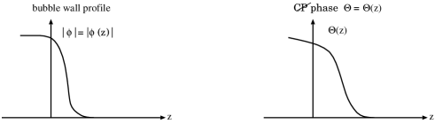
Figure 11: Sketch of the variation of the modulus and the CP-violating phase angle of a non-SM Higgs VEV, in the wall frame, at the boundary between the broken and the symmetric phase.

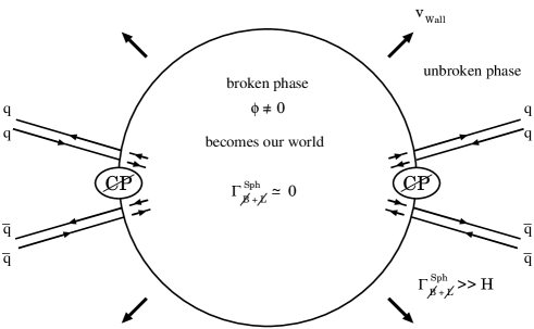
Figure 12: Sketch of nonlocal electroweak baryogenesis.

We consider for simplicity only the so-called thin wall regime which applies if the mean free path of a fermion, $l_{\psi}$, is larger than the thickness $l_{wall}$. Then the quarks and leptons can be treated as free particles, interacting only in a small region with a non-trivial Higgs background field, see Fig. 11. Multiple scattering within the wall may be neglected. The expansion of the wall is supposed to be spherically symmetric and the 1-dimensional description as given in section 5.3.1 applies. Fig. 13 shows left-handed and right-handed quarks $q_{L}$ and $q_{R}$ incident from the unbroken phase, which hit the moving wall and are reflected by the Higgs bubble into right-handed and left-handed quarks, respectively.

Figure 13: Reflection of left- and right-handed quarks at a radially expanding Higgs bubble. The transmission of (anti)quarks from the broken into the symmetric phase is not depicted.

In the frame where the wall is at rest, the fermion interactions with the bubble wall are described by the Dirac equation following from (72):

$$(i\gamma^{\mu}\partial_{\mu}-m(z)P_{R}-m^{*}(z)P_{L})\psi(z,t)\>=\>0\>,$$ (83)

where $P_{R,L}=(1\pm\gamma_{5})/2$ and $\psi$ is a c-number Dirac spinor. Solving this equation with the appropriate boundary conditions yields the (anti)quark wave functions of either chirality [61, 62].

Figure 14: The reflection $q_{L}\to q_{R}$ and the P-, CP-, and CPT-transformed process.

Instead of performing this calculation let’s make a few general considerations. Let’s have a look at the scattering process depicted in Fig. 14, where, in the symmmetric phase $z>z_{0}$, a left-handed quark $q_{L}$ (having momentum $k_{z}<0$) is reflected at the wall into a right-handed $q_{R}$. Notice that conservation of electric charge guarantees that a quark is reflected into a quark and not an antiquark. Angular momentum conservation tells us that $q_{L}$ is reflected as $q_{R}$ and vice versa. Also shown are the situations after a parity transformation (followed by a rotation around the wall axis in the paper plane orthogonal to the $z$ axis by an angle $\pi$), and subsequent charge conjugation C, and time reversal (T) transformations. The analogous figure can be drawn for antiquark reflection. These figures immediately tell us that if CP were conserved then

$${\cal R}_{L\to R}\>=\>{\cal R}_{{\bar{R}}\to{\bar{L}}}\>,\qquad{\cal R}_{R\to L}\>=\>{\cal R}_{{\bar{L}}\to{\bar{R}}}\qquad$$ (84)

would hold. (The subscripts ${\bar{R}}$, $\bar{L}$ denote right-handed and left-handed antiquarks, respectively.) CPT invariance, which is respected by the particle physics models we consider, implies

$${\cal R}_{L\to R}\>=\>{\cal R}_{{\bar{L}}\to{\bar{R}}}\>,\qquad{\cal R}_{R\to L}\>=\>{\cal R}_{{\bar{R}}\to{\bar{L}}}\>.\qquad$$ (85)

The charge transport mechanism [61] works as follows. At some initial time we have equal numbers of quarks and antiquarks in the unbroken phase, in particular equal numbers of $q_{L}$ and ${\bar{q}}_{R}$ and $q_{R}$ and ${\bar{q}}_{L}$, respectively, which hit the expanding bubble wall. Reflection converts $q_{L}\to q_{R}$, ${\bar{q}}_{R}\to{\bar{q}}_{L}$, $q_{R}\to q_{L}$, and ${\bar{q}}_{L}\to{\bar{q}}_{R}$ and the particles move back to the region where the Higgs fields are zero. Because the interaction with the bubble wall is assumed to be CP-violating, the relations (84) for the reflection probabilities no longer hold. Actually, for the CP asymmetry

$$\Delta{\cal R}_{CP}\>\equiv\>{\cal R}_{{\bar{L}}\to{\bar{R}}}-{\cal R}_{R\to L}\>=\>{\cal R}_{{L}\to{R}}-{\cal R}_{{\bar{R}}\to{\bar{L}}}$$ (86)

to be non-zero it is essential that $m_{q}(z)$ has a $z$ dependent phase. The reflection coefficients are built up by the coherent superposition of the amplitudes for (anti)quarks to reflect at some point $z$ in the bubble. When the phases vary with $z$ the reflection probabilities ${\cal R}_{{\bar{L}}\to{\bar{R}}}$ and ${\cal R}_{R\to L}$ differ from each other. If the phase of $m_{q}(z)$ were constant these probabilities would be equal. (Keep in mind that we work at the level of 1-particle quantum mechanics.) An explicit computation yields [63]

$$\Delta{\cal R}_{CP}(k_{z})\>\propto\>\int_{-\infty}^{+\infty}dz\,\cos(2k_{z}z){\rm Im}[m_{q}(z)M_{q}^{*}]\>,$$ (87)

where $M_{q}$ = $m_{q}(z=-\infty)$ is the mass of the quark in the broken phase, and $arg(M_{q})=\xi_{1}$ – see eq. (69). This equation corroborates the above statement; if $m_{q}(z)$ had a constant phase, the asymmetry would be zero. Notice that at this stage the net baryon number is still zero. This is because the difference $J_{q}^{L}$ of the fluxes of $\bar{q}_{R}$ and $q_{L}$, injected from the wall back into the symmetric phase, is equal to $J_{q}^{R}$ which we define as the difference of the fluxes of $q_{R}$ and ${\bar{q}}_{L}$, as should be clear from (85). However, the (B+L)-violating weak sphaleron interactions, which are unsuppressed in the symmetric phase away from the wall, act only on the (massless) left-handed quarks and right-handed antiquarks. For instance, the reaction (49) decreases the baryon number by 3 units, while the corresponding reaction with right-handed antiquarks in the initial state increases B by the same amount. Thus if the functional form of the CP-violating part ${\rm Im}[m_{q}(z)M_{q}^{*}]$ of the background Higgs field is such that $J_{q}^{L}>0$ then, after the anomalous weak interactions took place, there are more left-handed quarks than right-handed antiquarks. The fluxes of the reflected ${\bar{q}}_{L}$ and $q_{R}$ are not affected by the anomalous weak sphaleron interactions. Adding it all up we see that some place away from the wall a net baryon number $\Delta B>0$ is produced. Some instant later the expanding bubble sweeps over that region and the associated non-zero Higgs fields strongly suppress the (B+L)-violating back reactions that would wash out $\Delta B$. Thus the non-zero B number produced before is frozen in.

We must also take into account that (anti)particles in the broken phase can be transmitted into the symmetric phase and contribute to the (anti)particle fluxes discussed above. Using CPT invariance and unitarity, we find that the probabilities for transmission and the above reflection probabilities are related:

$${\mathcal{T}}_{L\to L}\>=\>1-{\cal R}_{R\to L}\>=\>1-{\cal R}_{{\bar{R}}\to{\bar{L}}}\>=\>{\mathcal{T}}_{{\bar{L}}\to{\bar{L}}}\>,$$ (88)

$${\mathcal{T}}_{R\to R}\>=\>1-{\cal R}_{L\to R}\>=\>1-{\cal R}_{{\bar{L}}\to{\bar{R}}}\>=\>{\mathcal{T}}_{{\bar{R}}\to{\bar{R}}}\>.$$ (89)

We can now write down a formula for the current $J_{q}^{L}$, which we define as the difference of the fluxes of $\bar{q}_{R}$ and $q_{L}$, injected from the wall into the symmetric phase. The contribution from the reflected particles involves the term $\Delta{\cal R}_{CP}f_{s}$ where $f_{s}$ is the free-particle Fermi-Dirac phase-space distribution of the (anti)quarks in the region $z>z_{0}$ that move to the left, i.e., towards the wall. The contribution from the (anti)quarks which have returned from the broken phase involves $({\cal T}_{{\bar{R}}\to{\bar{R}}}-{\cal T}_{L\to L})f_{b}=-\Delta{\cal R}_{CP}f_{b}$, where $f_{b}$ is the phase-space distribution of the transmitted (anti)quarks that move to the right. The reference frame is the wall frame. Notice that $f_{s}$ and $f_{b}$ differ because the wall moves with a velocity $v_{wall}\neq 0$ – in our convention from left to right. The current $J_{q}^{L}$ is given by

$$J_{q}^{L}\>=\>\int_{k_{z}<0}\,\frac{d^{3}k}{(2\pi)^{3}}\frac{|k_{z}|}{E}(f_{s}\,-\,f_{b})\Delta{\cal R}_{CP}\,,$$ (90)

where $|k_{z}|/E$ is the group velocity. The current is non-zero because two of the three Sakharov conditions, CP violation and departure from thermal equilibrium, are met. The current would vanish if the wall were at rest in the plasma frame – which leads to thermal equilibrium –, because then $(f_{s}-f_{b})=0$.

The current $J^{L}=\sum_{\psi}J_{\psi}^{L}$ is the source for baryogenesis some distance away from the wall as sketched above. We skip the analysis of diffusion and of the conditions under which local thermal equilibrium is maintained in front of the bubble wall [61, 63, 64]. This determines the densities of the left-handed quarks and right-handed antiquarks and their associated chemical potentials. The rate of baryon production per unit volume is determined by the equation [63]

$$\frac{dn_{B}}{dt}\>=\>-n_{F}\frac{\hat{\Gamma}_{sph}}{2T}\sum_{generations}(3\hat{\mu}_{U_{L}}+3\hat{\mu}_{D_{L}}+\hat{\mu}_{\ell_{L}}+\hat{\mu}_{\nu_{L}})\>,$$ (91)

where $n_{F}=3$, $U=u,c,t$, $D=d,s,b$, ${\hat{\Gamma}_{sph}}$ is the sphaleron rate per unit volume, which in the unbroken phase is given by eq. (53). Here the $\hat{\mu}_{i}=\mu_{i}-{\bar{\mu}_{i}}=2\mu_{i}$ denote the difference between the respective particle and antiparticle chemical potentials. For a non-interacting gas of massless fermions $i$, the relation between $\hat{\mu}_{i}$ and the asymmetry in the corresponding particle and antiparticle number densities is $n_{i}-{\bar{n}}_{i}\simeq g{\hat{\mu}_{i}}T^{2}/12$, where $g=1$ for a left-handed lepton and $g=3$ for a left-handed quark because of three colors. In the symmetric phase (91) then reads

$$\frac{dn_{B}}{dt}\>=\>-6n_{F}\frac{\hat{\Gamma}_{sph}}{T^{3}}(3B_{L}+L_{L})\>,$$ (92)

where $B_{L}$ and $L_{L}$ denote the total left-handed baryon and lepton number densities, respectively. The factor of 3 comes from the definition of baryon number, which assigns baryon number 1/3 to a quark. This equation tells us what we already concluded qualitatively above: baryon rather than antibaryon production requires a negative left-handed fermion number density, i.e., a positive flux $J_{q}^{L}$. The total flux $\sum_{\psi}J_{\psi}^{L}$ determines the left-handed fermion number density. Then eq. (92) yields $n_{B}$ and, using $s=2\pi^{2}g_{*s}T^{3}/45$ with $g_{*s}\simeq 110$ (see section 2.2), a prediction for the baryon-to-entropy ratio is obtained.

So much to the main aspects of the mechanism. There are, however, a number of issues that complicate this scenario. Decoherence effects during reflection should be studied. The propagation of fermions is affected by the ambient high temperature plasma leading to modifications of their vacuum dispersion relations. The shape and velocity of the wall is a critical issue. We refer to the quoted literature for a discussion of these and other points.

Because Higgs sector CP violation as discussed above is strongest for top quarks, one might expect that these quarks make the dominant contribution to the right hand side of (92). However, several effects tend to decrease their contribution relative to those of $\tau$ leptons. As top quarks interact much more strongly than $\tau$ leptons they have a shorter mean free path. This means that for typical wall thicknesses the thin-wall approximation does not hold for $t$ quarks. Further the injected left-handed top current $J_{t}^{L}$ is affected by QCD sphaleron fields which induce processes – unsuppressed at high $T$ – where the chiralities of the quarks are flipped [66, 67]. This damps the $t$ quark contribution to $B_{L}$. Refs. [63, 64] come to the conclusion that in this type of particle physics models the contribution of $\tau$ leptons to the left-handed fermion number density is the most important one. Ref. [64] finds that this induces a baryon-to-entropy ratio of about

$$\frac{n_{B}}{s}\>\simeq\>10^{-12}\frac{\Delta\theta}{v_{wall}}\>,$$ (93)

where $v_{wall}$ is the velocity of the wall and ${\Delta\theta}\simeq\theta(z=-\infty)-\theta(z=+\infty)$. Barring the possibility of spontaneous CP violation at non-zero temperatures in the 2-Higgs doublet models, $\Delta\theta$ should be roughly of the order of the CP-violating phase $\xi$ in the 2-doublet potential (64). Using that primordial nucleosynthesis allows $n_{B}/s\simeq\eta/7\simeq(2-8)\times 10^{-11}$ (cf. (26)) one gets the parameter constraint $\Delta\theta/v_{wall}\sim 40$. Even large CP violation, $\Delta\theta$ of order 1, would require small wall velocities, which might not be supported by investigations of the dynamics of the phase transition. Nevertheless, the 2-Higgs doublet models predict roughly the correct order of magnitude. In view of the complexity of this baryogenesis scenario, there are possibly additional, hitherto unnoticed effects that may influence $n_{B}/s$. For a treatment of the case when the bubble walls are thick, in the sense that fermions interact with the plasma many times as the wall sweeps through, see [65].

Only a few words on electroweak baryogenesis in the minimal supersymmetric standard model, see e.g. [53, 54, 55, 56]. The essentials of the scenario are analogous to the 2HDM case, with CP-violating sources as described in section 5.3.2, the main source for baryogenesis being the phase $\varphi_{\mu}$ of the complex Higgsino mixing parameter $\mu_{c}$. A number of authors conclude that the dominant baryogenesis source comes from the Higgsino sector, which produces a non-zero flux of left-handed quark chirality. The results for $n_{B}/s$ may be presented in the form

$$\frac{n_{B}}{s}\>=\>4\times 10^{-11}a\sin\varphi_{\mu}\>.$$ (94)

There is a considerable spread in the predicted values of $a$, respectively in the resulting estimates of the necessary magnitude of $\sin\varphi_{\mu}$. While refs. [54, 56] find that a small CP phase $\varphi_{\mu}\gtrsim 0.04$ would suffice to obtain the correct order of magnitude of $n_{B}/s$ (which requires, however, small wall velocities), ref. [55] concludes that $\sin\varphi_{\mu}$ must be of order 1. Large values of $\varphi_{\mu}$ , however, tend to be in conflict with the constraints from the experimental upper bounds on the electric dipole moments of the electron and neutron, see section 5.3.2. Electroweak baryogenesis in a next-to-minimal SUSY model was investigated in [68].

5.5 Role of the KM Phase

We haven’t yet discussed which role is played in baryogenesis scenarios by the SM source of CP violation, the KM phase $\delta_{KM}$. This question was put out of the limelight after it had become clear that the SM alone cannot explain the BAU, for reasons outlined above. Therefore, SM extensions must be invoked, and such extensions usually entail in a natural way new sources of CP violation which can be quite effective, as far as their role in baryogenesis scenarios is concerned, as we have seen – see also the next section. Nevertheless, this is a very relevant issue.

Recall the following well-known features of KM CP violation. All CP-violating effects, which are generated by the KM phase in the charged weak quark current couplings to W bosons, are proportional to the invariant [69, 70]:

$$J_{CP}\>=\>\prod_{i>j\atop u,c,t}(m^{2}_{i}-m^{2}_{j})\prod_{i>j\atop d,s,b}(m^{2}_{i}-m^{2}_{j})\quad{\rm Im}\,Q\>,$$ (95)

where i,j = 1,2,3 are generation indices, $m_{u}$, etc. denote the respective quark masses, and ${\rm Im}\,Q$ is the imaginary part of a product of 4 CKM matrix elements, which is invariant under phase changes of the quark fields. There are a number of equivalent choices for ${\rm Im}\,Q$. A standard choice is

$${\rm Im}\,Q={\rm Im}(V_{ud}V_{cb}V^{*}_{ub}V^{*}_{cd})\>.$$ (96)

Inserting the moduli of the measured CKM matrix elements yields $|{\rm Im}\,Q|$ smaller than $2\times 10^{-5}$, even if KM CP violation is maximal; i.e., $\delta_{KM}=\pi/2$ in the KM parameterization of the CKM matrix. We may write ${\rm Im}\,Q\simeq 2\times 10^{-5}\sin\delta_{KM}$. As far as the SM at temperatures $T\neq 0$ is concerned, the CP symmetry can be broken only in regions of space where the gauge symmetry is also broken, or at the boundaries of such regions, because $J_{CP}\neq 0$ requires non-degenerate quark masses. Imagine the EW transition would be first order due to a 2-Higgs doublet extension of the SM with no CP violation in the Higgs sector. The question is then: is the KM source of CP violation strong enough to create a sufficiently large asymmetry $\Delta{\cal R}_{CP}$ in the probabilities for reflection of (anti)quarks at the expanding wall as discussed above? It is clear that $\Delta{\cal R}_{CP}$ must be proportional to a dimensionless quantity of the form $J_{CP}/D$, where $D$ has mass dimension 12. Reflection of quarks and antiquarks at a bubble wall is not CKM-suppressed; hence $D$ does not contain small CKM matrix elements. If one recalls that in the symmetric phase the quark masses and thus $J_{CP}$ vanish, it seems reasonable to treat the quark masses (perhaps not the top quark mass) as a perturbation. In the massless limit the mass scale of the theory at the EW transition is then given by the critical temperature $T_{c}\sim$ 100 GeV. Thus one gets for the dimensionless measure of CP violation:

$$d_{CP}\>\equiv\>\frac{J_{CP}}{T_{c}^{12}}\>\sim\>10^{-19}\>$$ (97)

as an estimate of $\Delta{\cal R}_{CP}$. Clearly this number is orders of magnitude too small to account for the observed $n_{B}/s$. CP violation à la KM is therefore classified, by consensus of opinion, as being irrelevant for baryogenesis. It was argued, however, that there may exist significant enhancement effects [71], and there has been a considerable debate over this issue [71, 72, 73].

6 Out-of-Equilibrium Decay of Super-Heavy Particle(s)

Historically the first type of baryogenesis scenario which was developed in detail is the so-called out-of-equilibrium decay of a super-heavy particle [74, 75, 16, 76]. The basic idea is that at a very early stage of the expanding universe, a super-heavy particle species $X$ existed, the reaction rate of which became smaller than the expansion rate $H$ of the universe at temperatures $T\gg T_{EW}$. Therefore, these particles decoupled from the thermal bath and became over-abundant. The decays of $X$ and of the antiparticles $\bar{X}$ are supposed to be CP- and B-violating, such that a net baryon number $\Delta B\neq 0$ is produced when the $X,\bar{X}$ have decayed. This scenario has its natural setting in the framework of grand unified theories. A brief outline is given in the next subsection. A viable variant is baryogenesis via leptogenesis through the lepton-number violating decays of (a) heavy Majorana neutrino(s) [77]. This will be discussed in subsection 6.2.

6.1 GUT Baryogenesis

The “out-of-equilibrium decay” scenario is natural in the context of grand unified theories. Grand unification aims at unifying the strong and electroweak interactions at some high energy scale. It works, for instance, in the context of supersymmetry, where the effective couplings of the strong, weak, and electromagnetic interactions become equal at an energy scale $M_{GUT}\simeq 10^{16}$ GeV [47]. A matter multiplet forming a representation of the GUT gauge group $G$ contains both quarks and leptons. Gauge bosons mediate transitions between the members of this multiplet, and – for many gauge groups – some of the gauge bosons induce B-violating processes. Also C violation and non-standard CP violation occurs naturally. As to the latter: the gauge group $G$ must be broken at the GUT scale $M_{GUT}\simeq 10^{16}$ GeV to some smaller symmetry group $G^{\prime}\supseteq SU(3)_{c}\times SU(2)_{L}\times U(1)_{Y}$. This is accomplished by scalar Higgs multiplets. As a consequence, GUTs contain in general super-heavy Higgs bosons with B-violating and CP-violating Yukawa couplings to quarks and leptons.

The simplest example of a GUT is based on the gauge group $G=SU(5)$. It is obsolete because the model is in conflict with the stability of the proton. Irrespective of this obstruction the minimal version of this model is of no use for implementing the scenario which we discuss below, because the interactions of minimal $SU(5)$ conserve $B-L$. A popular gauge group is $SO(10)$ which allows to construct models that avoid both obstacles [47].

Rather than going into the details of a specific GUT let us illustrate the baryogenesis mechanism with a well-known toy model [1]. Consider a super-heavy leptoquark gauge boson $X$ which is supposed to have quark-quark and quark-lepton decay channels, $X\to qq,{\ell}{\bar{q}}$. In the table the branching ratios of these decays, of the decays of the antiparticle $\bar{X}$, and the baryon numbers $B$ of the final states are tabulated.

final state $f$	branching ratio	$B$
$X\to qq$	$r$	2/3
$X\to{\ell}{\bar{q}}$	$1-r$	-1/3
${\bar{X}}\to{\bar{q}}{\bar{q}}$	${\bar{r}}$	-2/3
${\bar{X}}\to{\bar{\ell}}{q}$	${1-\bar{r}}$	1/3

The baryon number produced in the decays of $X$ and $\bar{X}$ is:

$$B_{X}\>=\>\frac{2}{3}r-\frac{1}{3}(1-r)\>,$$

$$B_{\bar{X}}\>=\>-\frac{2}{3}{\bar{r}}+\frac{1}{3}(1-{\bar{r}})\>,$$ (98)

and the net baryon number produced is

$$\Delta B_{X} \equiv B_{X}+B_{\bar{X}}=r-{\bar{r}}$$ (99)

$$= \frac{\Gamma(X\to f_{1})}{\Gamma_{tot}(X)}-\frac{\Gamma({\bar{X}}\to{\bar{f}_{1}})}{\Gamma_{tot}(\bar{X})}=\frac{\Gamma(X\to f_{1})-\Gamma({\bar{X}}\to{\bar{f}_{1}})}{\Gamma_{tot}}\>,$$

where $f_{1}=qq$ and we have used that ${\Gamma_{tot}(X)}={\Gamma_{tot}(\bar{X})}$, which follows from CPT invariance. Obviously if C or CP were conserved then $\Delta B_{X}=0$. Suppose the quarks and leptons $q,\ell$ couple to a spin-zero boson $\chi$ with Yukawa couplings that contain a non-removable CP-violating phase. It is natural to assume that C is already violated in the tree-level interactions of $X$ to fermions. The CP-violating interactions affect the $X,\bar{X}$ decay amplitudes beyond the tree level, as shown in Fig. 15. The decay amplitude for $X\to qq$ is, up to spinors and a polarization vector describing the external particles,

$$A(X\to qq)\>=\>A_{0}+A_{1}=A_{0}+Be^{i\delta_{CP}}\>,$$ (100)

where the tree amplitude $A_{0}$ is real. $\Delta B_{X}\neq 0$ requires, in addition to CP violation, also a non-zero final-state interaction phase. Therefore, the masses of the $X$ boson and of the fermions must be such that the intermediate fermions in the 1-loop contribution to the amplitude can be on their respective mass shells and re-scatter to produce the final state. This causes a complex $B=|B|\exp(i\omega)$. The decay amplitude for ${\bar{X}}\to{\bar{q}}{\bar{q}}$ is

$$A({\bar{X}}\to{\bar{q}}{\bar{q}})\>=\>A_{0}+|B|e^{i\omega}e^{-i\delta_{CP}}\>.$$ (101)

Using (100), (101) one obtains that

$$\Delta B_{X}\>\propto\>\frac{|AB|\sin\omega\sin\delta_{CP}}{\Gamma_{tot}}\>,$$ (102)

and the constant of proportionality includes factors from phase space integration. In addition, the baryon number $\Delta B_{\chi}$ produced in the decays of the $\chi,\bar{\chi}$ bosons must also be computed. Let’s assume that $\Delta B_{X}+\Delta B_{\chi}\neq 0.$

Figure 15: Amplitude for the decay $X\to qq$ to one-loop approximation. The vertical dashed line indicates the absorptive part of the 1-loop contribution which enters $\Delta B_{X}$.

As long as the interactions of these bosons, which include decays, inverse decays, annihilation, the B-violating reactions $qq\to\ell{\bar{q}}$, ${\bar{q}}{\bar{q}}\to{\bar{\ell}}{q}$, etc. (remember the discussion in section 3.2) are fast compared to the expansion rate $H$, the $X,\bar{X},\chi,\bar{\chi}$ have thermal distributions and the average baryon number of the plasma remains zero. Therefore the interactions of these bosons must be weak enough that they can fall out of equilibrium. This is a delicate issue, because these particles carry gauge charges and can couple quite strongly to the plasma of the early universe.

Let’s outline the scenario for the $X,\bar{X}$. (It applies also to the scalar particles.) At temperatures $T\gg m_{X}$, where $m_{X}$ is the mass of the $X$ boson, the $X,{\bar{X}}$ particles have relativistic velocities and are assumed to be in thermal equilibrium. Then $n_{X}=n_{\bar{X}}\sim n_{\gamma}$ holds for their number densities. At lower temperatures, the $X,{\bar{X}}$ bosons become non-relativistic and, as long as they remain in thermal equilibrium, their densities get Boltzmann-suppressed with decreasing temperature, $n_{\bar{X}}=n_{X}\sim(m_{X}T)^{3/2}\exp(-m_{X}/T)$. Because $\Gamma_{annih}\propto n_{X}$, the total rate $\Gamma_{X}\sim\alpha m_{X}$ of $X$ and $\bar{X}$ decay is the relevant number to compare with $H$. If $\Gamma_{X}<H$, an excess of $X,\bar{X}$ with respect to their equilibrium numbers will develop. The $X,\bar{X}$ drift along in the expanding universe for a little while and decay. Notice that the inverse decays, $f\to X$, ${\bar{f}}\to{\bar{X}}$, by which bosons are created again by quark-quark annihilation, etc. are blocked, because the fraction of these fermions with sufficient energy to produce a super-heavy boson is Boltzmann suppressed for $T<m_{X}$. At the time of their decay, $t\sim\Gamma_{X}^{-1}$, there is quite an over-abundance: $n_{X}=n_{\bar{X}}\sim n_{\gamma}(T_{decay})$. Using that the entropy density $s\sim g_{*}n_{\gamma}$ (see sect. 2.2) one gets for the produced baryon asymmetry:

$$\frac{n_{B}}{s}\>\sim\>\frac{\Delta B\,n_{\gamma}}{g_{*}n_{\gamma}}\>\sim\>\frac{\Delta B}{g_{*}}\>,$$ (103)

where $\Delta B\simeq\Delta B_{X}$ is the baryon number produced per boson decay. For a (GUT) extension of the SM one may expect that $g_{*}$ is somewhere between $10^{2}$ and $10^{3}$. Thus only a tiny CP asymmetry $\Delta B\sim 10^{-8}-10^{-7}$ is required to obtain $n_{B}/s\sim 10^{-10}$. Of course, these crude estimates must be made quantitative by computing the relevant reaction rates using a specific particle physics model, and tracking the time evolution of the particle densities by solving the Boltzmann equations. A detailed exposition is given in [1].

The above condition for the decoupling of the $X$ particles from the thermal bath, $\Gamma_{X}\sim\alpha m_{X}<H$, translates into a condition on the mass of the spin 1 gauge boson: $m_{X}>\alpha g_{*}^{-1/2}m_{Pl}\sim 10^{16}$ GeV, where $\alpha=g_{gauge}^{2}/(4\pi)\sim 10^{-2}$. For super-heavy scalar bosons with B-violating decays a mass bound obtains which is lower (cf., e.g., [6]).

There are several pitfalls that constrain this type of baryogenesis mechanism. First, remember that a scenario that tries to explain the BAU by a mechanism that operates above the temperature $T_{EW}\sim 100$ GeV must involve interactions that violate $B-L$. In the context of grand unified theories, models based on the gauge group $SO(10)$ lead to $(B-L)$ non-conservation. These models have several attractive features, in particular with respect to the scenario discussed in the next subsection.

GUT baryogenesis may be in conflict with inflation. This is a serious problem. An essential assumption in the above scenario was that at very high temperatures $T$ above $m_{X}$ the $X,\bar{X}$ particles were in thermal equilibrium and were as abundant as photons. If these particles are the super-heavy gauge or Higgs bosons of a GUT this assumption may be wrong. It might be that the temperature of the quasi-adiabatically expanding plasma of particles in the early universe was always smaller than $M_{GUT}$. There are a number of reasons to believe that the energy of the very early universe was dominated by vacuum energy, which led to exponential expansion of the cosmos. This is the basic assumption of the inflationary model(s). These models solve a number of fundamental cosmological problems, including the monopole problem. A number of GUTs predict super-heavy, stable magnetic monopoles. Their contribution to the energy density of the universe would over-close the cosmos – but that is not observed. Inflation would sweep away these monopoles, along with other particles, leaving an empty space. At the end of inflation the vacuum energy is converted through quantum fluctuations into pairs of relativistic particles and antiparticles which then thermalize. This process is called reheating and it can be characterized by an energy scale called the reheat temperature $T_{r}$. If the reheating process is fast, i.e., if $T_{r}$ is above $M_{GUT}$, the monopoles are re-created. On the other hand if reheating occurred slowly such that $T_{r}$ is well below $M_{GUT}$ then the re-production of $X\bar{X}$ super-heavy gauge and Higgs bosons – which were to initiate baryogenesis as described above – appears to be inhibited, or should at least be suppressed. See [6] for an overview on ways to circumvent this and associated problems.

6.2 Baryogenesis through Leptogenesis

This mechanism is a special case of the “out-of-equilibrium decay” scenario. It assumes the existence of a heavy Majorana neutrino species in the early universe above $T_{EW}$ with a particle mass, typically, of the order of $M\sim 10^{12}$ GeV – or, in fact, the more realistic case of three heavy Majorana neutrino species with non-degenerate masses. These particles interact only weakly with the other particle species in the early universe and fall out of equilibrium at some temperature $T\sim M\gg T_{EW}$. It is essential that some of the interactions of the underlying particle physics model do not conserve $B-L$. The heavy Majorana neutrinos decay, for instance into ordinary leptons and Higgs bosons which are the most important channels, thereby generating a non-zero lepton number. Lepton-number violating scattering processes must not wash out this asymmetry. Then the $(B-L)$-conserving SM sphaleron reactions, which occur rapidly enough above $T_{EW}$, convert this lepton asymmetry into a baryon asymmetry.

The scenario was suggested in [77], and it has been subsequently developed further – see [78, 79, 80, 82, 81, 83] and the reviews [7]. The attractiveness of this scenario stems from the observed atmospheric and solar neutrino deficits which point to oscillations of the light neutrinos. It is well-known that these data can be explained by small differences in the masses of the electron, muon, and tau neutrinos. The value of $\Delta m^{2}_{23}=m^{2}_{3}-m^{2}_{2}$ extracted from the data indicates that the mass of the heaviest of the three light neutrinos is of the order of $10^{-2}$ eV. Such small masses can be explained in a satisfactory way by the so-called seesaw mechanism [84]. This mechanism requires (i) the neutrinos to be Majorana fermions and (ii) three very heavy right-handed neutrinos which are singlets with respect to $SU(2)_{L}\times U(1)_{Y}$ – see Appendix B.

Within the framework of GUTs, popular models are based on the gauge group $SO(10)$ which contain in their particle spectra ultra-heavy right-handed Majorana neutrinos with lepton-number violating decays. We consider here only a minimal, non-GUT model. Take the electroweak standard model and add three right-handed $SU(2)_{L}\times U(1)_{Y}$ singlet fields $\nu_{\alpha R}$ $(\alpha=1,2,3)$ with a Majorana mass term for these fields involving mass parameters much larger than $v=246$ GeV. The general Yukawa interaction for the charged leptons and neutrinos is then given by eq. (149) of appendix B with $\Phi\equiv\Phi_{1}=\Phi_{2}$, where $\Phi=(\phi^{+},\phi^{0})^{T}$ is the SM $SU(2)_{L}$ doublet field. As described in appendix B we have in the mass basis three very light, practically left-handed Majorana neutrinos, which we identify with the neutrinos we know, and three very heavy, right-handed Majorana neutrinos $N_{i}$. Let’s switch back to the early universe when the $N_{i}$ were still around. The interaction (149) implies that the $N_{i}$ have lepton-number violating decays at tree-level, $N_{i}\to\ell\phi$ and $N_{i}\to{\bar{\ell}}\phi^{*}$, where $\ell,\phi$ denotes either a negatively charged lepton and a $\phi^{+}$ (which later ends up as the longitudinal component of the $W^{+}$ boson) or a light neutrino and a $\phi^{0}$. C and CP violation cause a difference in these two rates – see below. As long as the $N_{i}$ are in thermal equilibrium CPT invariance and the unitarity of the S matrix ( cf. section 3.2) guarantee that the average lepton number remains zero. (The $N_{i}$ are to be described as on-shell resonances in corresponding $2\leftrightarrow 2$ processes.) When the $N_{i}$ have fallen out of equilibrium, there is still the danger of lepton-number violating wash-out processes, for instance ${|\Delta L|=2}$ reactions mediated by $N_{i}$ exchange. The requirement $\Gamma_{|\Delta L|=2}(T)<H(T)$ for temperatures $T$ smaller than the leptogenesis temperature, e.g. $T\lesssim 10^{10}$ GeV, implies an upper bound on the masses of the light neutrinos [7].

We assume the $N_{i}$ to be non-degenerate and put the labels such that $M_{3}>M_{2}>M_{1}$ holds for the masses. The decay width of $N_{i}$ at tree level in its rest frame, see Fig. 16, is easily computed using (149):

$$\Gamma_{i} \equiv \Gamma(N_{i}\to\ell\phi)+\Gamma(N_{i}\to{\bar{\ell}}\phi^{*})$$ (104)

$$=\frac{(M_{D}^{\dagger}M_{D})_{ii}}{4\pi v^{2}}M_{i}\>,$$

where $M_{D}$ is the Dirac mass matrix (150). For leptogenesis to work the decays of the $N_{i}$ must be slow as compared to $H$. The condition $\Gamma_{i}<H(T=M_{i})$ is fulfilled only if the masses of the light neutrinos are small, roughly $m_{\nu_{i}}<10^{-3}$ eV [85], which is compatible with observations. There is then an excess of the heavy neutrinos with respect to their rapidly decreasing equilibrium distributions $n_{eq}\sim\exp(-M/T)$.

Figure 16: Two-body decay of a super-heavy Majorana neutrino $N_{1}\to\ell\phi$: Born amplitude (a) and a 1-loop contribution (b). Self-energy contributions are not depicted.

Eventually the $N_{i}$ decay and lepton number is produced. It is due to the CP-asymmetry in the decay rates which is generated by the interference of the tree amplitude with the absorptive part of the 1-loop amplitude depicted in Fig. 16, analogous to eq. (102). If $M_{1}\ll M_{2},M_{3}$ one obtains for the decay of $N_{1}$:

$$\epsilon_{1} \equiv \frac{\Gamma(N_{1}\to\ell\phi)-\Gamma(N_{1}\to{\bar{\ell}}\phi^{*})}{\Gamma(N_{1}\to\ell\phi)+\Gamma(N_{1}\to{\bar{\ell}}\phi^{*})}$$ (105)

$$\simeq-\frac{3}{4\pi v^{2}}\frac{1}{(M_{D}^{\dagger}M_{D})_{11}}\sum_{j=2,3}{\rm Im}[(M_{D}^{\dagger}M_{D})^{2}_{1j}]\frac{M_{1}}{M_{j}}\>.$$

The asymmetries $\epsilon_{i}$ are determined by the moduli and the CP-violating phases of the elements of the matrix $M_{D}^{\dagger}M_{D}$. The moduli are related to the light neutrino masses, while the CP-violating phases are in general unrelated to the CP-violating phases of the mixing matrix in the leptonic charged current-interactions involving the light neutrinos – see appendix B.

The asymmetry (105) corresponds to an asymmetry in the density of leptons versus antileptons, $n_{L}\equiv n_{\ell}-n_{\bar{\ell}}\neq 0.$ A crude estimate of the lepton-number-to-entropy ratio $Y_{L}=n_{L}/s$ gives

$${Y_{L}}\>\sim\>\epsilon_{1}\frac{n_{N}}{s}\>\sim\>\frac{\epsilon_{1}}{g_{*}}\>,$$ (106)

where $g_{*}\sim 100$ in the SM. Due to wash-out processes like those mentioned above this ratio is, in fact, smaller than (106). In order to determine the suppression factor $\kappa$, the Boltzmann equations for the time evolution of the particle number densities must be solved [78, 80, 7]. A typical solution for $n_{N_{1}}$ is sketched in Fig. 17. Refs. [80, 7] find $\kappa\sim 10^{-1}-10^{-3}$, depending on the particle physics model.

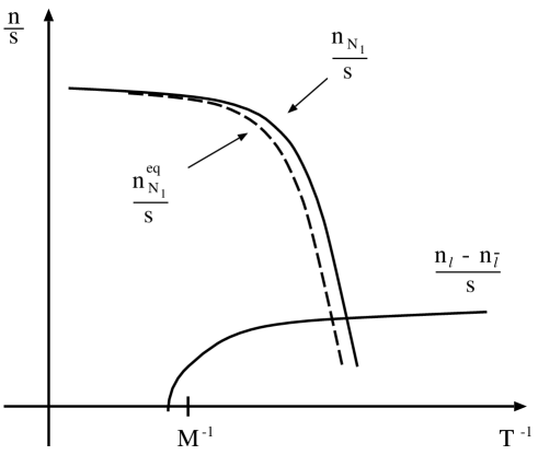
Figure 17: Evolution of the ratio $n_{N_{1}}/s$ as the universe cools off. Departure from thermal equilibrium occurs at $T\lesssim M_{N_{1}}$ and a leptonic asymmetry is generated [7].

The asymmetry in lepton number feeds the $(B-L)$-conserving weak sphaleron reactions, which occur rapidly enough above $T_{EW}$, and produce an asymmetry in baryon number $Y_{B}=n_{B}/s$. There is a relation between $Y_{B}$ and the corresponding asymmetries $Y_{B-L}$ and $Y_{L}$. For a given particle physics model this relation depends on the processes which are in thermal equilibrium, and it is given by [86, 87]:

$${Y_{B}}\>=\>C\,Y_{B-L}\>=\>\frac{C}{C-1}\,Y_{L}\>.$$ (107)

The particle reactions which are fast enough as compared with $H$ yield relations among the various chemical potentials, and these relations determine the number $C$. For the minimal model considered above, one has $C=28/79$ in the high temperature phase if all but the $|\Delta L|=2$ reactions are in thermal equilibrium [86]. (In general $C$ depends on the ratio $v_{T}/T$, where $v_{T}$ is the Higgs VEV which develops in the broken phase [88, 89].) Using (106), (107) the generated baryon-to-entropy ratio is estimated to be

$${Y_{B}}\>\sim-Y_{L}\>=\>-\kappa\frac{\epsilon_{1}}{g_{*}}\>.$$ (108)

Using $g_{*}\sim 100$ and a dilution factor $\kappa\sim 10^{-2}$, we see that only a very small lepton-asymmetry $\epsilon_{1}\sim 10^{-6}$ is needed. In fact, lepton-number violation must not be too strong, in order that the whole scenario works.

Detailed studies of leptogenesis have been made, for a number of SM extensions and using Ansätze for the neutrino mass matrices that fit well to the observations concerning the solar and atmospheric neutrino deficits [7]. The conclusion is that ${Y_{B}}\sim 10^{-10}$ is naturally explained by the decay of heavy Majorana neutrinos, the lightest of which having a mass $M_{1}\sim 10^{10}$ GeV, and the required pattern of the 3 light neutrino masses is consistent with observations.

7 Summary

In these lectures I have outlined two popular theories of baryogenesis, which presently seem to be the most plausible ones: electroweak baryogenesis and out-of-equilibrium decay scenarios, in particular baryogenesis via leptogenesis by the decays of ultra-heavy Majorana neutrinos. A number of other, quite ingenious mechanisms for generating the BAU were conceived. Their discussion is, however, beyond the scope of these notes and the reader is referred to the quoted reviews.

Electroweak baryogenesis (EWBG) will be testable in the not too distant future. The clarification of the origin of electroweak symmetry breaking will be a central physics issue at the Tevatron and at future colliders, and the outcome will be crucial for the EWBG scenario. An important result was already obtained: Theoretical investigations of the SM electroweak phase transition and the experimental lower bound from the LEP experiments on the mass of the SM Higgs boson, $m_{H}^{SM}>114$ GeV, led to the conclusion that the standard model of particle physics fails to explain the BAU. EWBG is still viable in extensions of the SM, the most popular of which is the minimal supersymmetric extension. However, the requirement of the electroweak phase transition to be strongly first order translates into tight upper bounds on the mass of the lightest Higgs boson, $m_{H}<115$ GeV, and on the mass of the lighter of the two stop particles, $m_{\tilde{t}_{1}}<170$ GeV, of the MSSM. Another important ingredient to EWBG is non-standard CP violation. This motivates the search for T-violating effects in experiments with atoms and molecules, and neutrons. Non-SM CP violation can also be traced in B meson decays or in high-energy reactions including the production and decays of top quarks and Higgs bosons, if Higgs particles will be discovered.

GUT-type baryogenesis scenarios cannot be falsified by laboratory experiments, but they would, of course, get spectacular empirical support if proton decay would be found, etc. That’s what makes leptogenesis by the decays of ultra-heavy Majorana neutrinos attractive: it has, albeit indirect, support from the observed atmospheric and solar neutrino deficits. Theoretical investigations have shown that the scenario is consistent. As far as unknown parameters are concerned, the degree of arbitrariness is constrained: in order to obtain the correct order of magnitude of the BAU the masses of the light neutrinos must lie in range which is consistent with the interpretation of the solar and atmospheric neutrino data. The scenario would get a further push if the light neutrinos would turn out to be Majorana particles. Future particle physics experiments and/or astrophysical observations will bring us closer to understanding what is responsible for the matter-antimatter asymmetry of the universe.

Acknowledgments

I wish to thank M. Beyer and A. Brandenburg for comments on the manuscript and I am indebted to T. Leineweber for the production of the postscript figures.


Appendix A

Let $q({\bf x},t)$ be the Dirac field operator that describes a quark of flavor $q=u,...,t$, $q^{\dagger}({\bf x},t)$ denotes its Hermitean adjoint, and ${\bar{q}}=q^{\dagger}\gamma^{0}$. The baryon number operator (36) is

$$\hat{B}=\frac{1}{3}\sum_{q}\int d^{3}x:q^{\dagger}({\bf x},t)q({\bf x},t):\>,$$ (109)

and the colons denote normal ordering. Let C, P denote the unitary and T the anti-unitary operator which implement the charge conjugation, parity, and time reversal transformations, respectively, in the space of states. Their action on the quark fields is, adopting standard phase conventions,

$$Pq({\bf x},t)P^{-1} = \gamma^{0}q({-\bf x},t)\,,$$ (110)

$$Pq^{\dagger}({\bf x},t)P^{-1} = q^{\dagger}({-\bf x},t)\gamma^{0}\,,$$ (111)

$$Cq({\bf x},t)C^{-1} = i\gamma^{2}q^{\dagger}({\bf x},t)\,,$$ (112)

$$Cq^{\dagger}({\bf x},t)C^{-1} = iq({\bf x},t)\gamma^{2}\,,$$ (113)

$$Tq({\bf x},t)T^{-1} = -i\ q({\bf x},-t)\gamma_{5}\gamma^{0}\gamma^{2}\,,$$ (114)

$$Tq^{\dagger}({\bf x},t)T^{-1} = -i\gamma^{2}\gamma^{0}\gamma_{5}q^{\dagger}({\bf x},-t)\,,$$ (115)

where $\gamma^{0}$, $\gamma^{2}$, and $\gamma_{5}=i\gamma^{0}\gamma^{1}\gamma^{2}\gamma^{3}$ denote Dirac matrices. Then

$$P:q^{\dagger}({\bf x},t)q({\bf x},t):P^{-1}\>=\>:q^{\dagger}({-\bf x},t)q({-\bf x},t):\,,$$ (116)

$$C:q^{\dagger}({\bf x},t)q({\bf x},t):C^{-1}\>=\>:q({\bf x},t)q^{\dagger}({\bf x},t):\>=\>-:q^{\dagger}({\bf x},t)q({\bf x},t):\,,$$ (117)

$$T:q^{\dagger}({\bf x},t)q({\bf x},t):T^{-1}\>=\>:q^{\dagger}({\bf x},-t)q({\bf x},-t):\,.$$ (118)

With these relations we immediately obtain:

$$P{\hat{B}}P^{-1} = {\hat{B}}\>,$$ (119)

$$C{\hat{B}}C^{-1} = -{\hat{B}}\>.$$ (120)

As shown in section 4 the baryon number operator is time-dependent due to non-perturbative effects. Using translation invariance we have ${\hat{B}(t)}=e^{iHt}{\hat{B}(0)}e^{-iHt}$, where $H$ is the Hamiltonian of the system. The operator ${\hat{B}(0)}$ is even with respect to T and odd with respect to $\Theta\equiv CPT$:

$$\Theta{\hat{B}(0)}{\Theta}^{-1}\>=\>-{\hat{B}(0)}\>.$$ (121)

Appendix B

Here we discuss the general structure of $SU(2)_{L}\times U(1)_{Y}$ invariant Yukawa interactions in the lepton sector if neutrinos are Majorana particles. Let’s first collect some basic formulae for Majorana fields. Consider a Dirac field

$$\psi(x)\>=\>\left(\begin{array}[]{c}\xi(x)\\ \eta(x)\end{array}\right)\,,$$ (122)

where $\xi,\eta$ are 2-component spinor fields. In the chiral representation of the $\gamma$ matrices, using the convention where $\gamma_{5}={\rm diag}({\rm I}_{2},-{\rm I}_{2})$, we have $\xi=\psi_{R},\eta=\psi_{L}$, where $\psi_{R},\psi_{L}$ are the right-handed and left-handed Weyl fields. In the chiral representation the charge conjugated spinor field $\psi^{c}$ reads

$$\psi^{c}\>\equiv\>i\gamma^{2}\psi^{\dagger}\>=\>\left(\begin{array}[]{c}i\sigma_{2}\eta^{\dagger}\\ -i\sigma_{2}\xi^{\dagger}\end{array}\right)\,,$$ (123)

and $\sigma_{2}$ is the second Pauli matrix. Let’s use the Weyl fields in 4-component form, $\psi_{R}=(\xi,0)^{T},\psi_{L}=(0,\eta)^{T}$, and determine, using (123), their charge-conjugates:

$$\psi^{c}_{L}\> \equiv \>(\psi_{L})^{c}\>=\>\left(\begin{array}[]{c}i\sigma_{2}\eta^{\dagger}\\ 0\end{array}\right)\,,$$ (126)

$$\psi^{c}_{R}\> \equiv \>(\psi_{R})^{c}\>=\>\left(\begin{array}[]{c}0\\ -i\sigma_{2}\xi^{\dagger}\end{array}\right)\,.$$ (129)

From this equation we can also read off the relation between the 2-component Weyl fields and their charge conjugates. Eq. (129) tells us that $\psi^{c}_{L}(\psi^{c}_{R})$ is a right-handed (left-handed) Weyl field. Thus the Weyl field operator $\psi_{L}(\psi_{R})$ annihilates a Dirac fermion state $|\psi>$ having L (R) chirality and creates an antifermion state $|{\bar{\psi}}>$ with R (L) chirality, while $\psi^{c}_{L}(\psi^{c}_{R})$ annihilates $|{\bar{\psi}}>$ having R (L) chirality and creates a state $|\psi>$ with L (R) chirality. Moreover, we immediately obtain that

$${\overline{\psi^{c}_{L}}}\> \equiv \>(\psi^{c}_{L})^{\dagger}\gamma^{0}\>=\>(0,\>i\eta^{T}\sigma_{2})\,,$$ (130)

$${\overline{\psi^{c}_{R}}}\> \equiv \>(\psi^{c}_{R})^{\dagger}\gamma^{0}\>=\>(-i\xi^{T}\sigma_{2},\>0)\,.$$ (131)

As to neutrinos, there are two options concerning their nature (which must eventually be resolved experimentally): either Dirac or Majorana fermion. The latter means, loosely speaking, that a neutrino would be its own antiparticle. Actually, for a Majorana fermion the distinction between particle and antiparticle looses its meaning because there is no longer a conserved quantum number that would discriminate between them (see below). A Majorana field is defined by the condition

$$\psi^{c}\>\stackrel{{\scriptstyle!}}{{=}}\>r\psi\>,$$ (132)

where $|r|=1$ is a phase chosen by convention. For $r=+1$ the four-component field $\psi_{1}=(i\sigma_{2}\eta^{\dagger},\,\eta)^{T}$ is a solution of this equation. In terms of Weyl fields this solution reads

$$\psi_{1}\>=\>\psi_{L}\>+\>\psi^{c}_{L}\,.$$ (133)

The other solution of eq. (132) with $r=1$ is

$$\psi_{2}\>=\>\psi_{R}\>+\>\psi^{c}_{R}\,.$$ (134)

Next we consider the Majorana mass terms. For Majorana particles described by $\psi_{1}$ and $\psi_{2}$ with masses $m_{1}$ and $m_{2}$, respectively, we can write down the following Majorana mass terms

$${\cal L}^{(1)}_{M}\> = \>-\frac{m_{1}}{2}{\bar{\psi}_{1}}\psi_{1}\>=\>-\frac{m_{1}}{2}{\overline{\psi^{c}_{L}}}\psi_{L}\>+\>{\rm h.c.}\>,$$ (135)

$${\cal L}^{(2)}_{M}\> = \>-\frac{m_{2}}{2}{\bar{\psi}_{2}}\psi_{2}\>=\>-\frac{m_{2}}{2}{\overline{\psi^{c}_{R}}}\psi_{R}\>+\>{\rm h.c.}\>,$$ (136)

where we have used that ${\bar{\psi}_{A}}\psi_{A}={\overline{\psi^{c}_{A}}}\psi^{c}_{A}=0$ for A=L,R. These mass terms violate the “$\psi$-number” by 2 units, $|\Delta{\rm L}_{\psi}|=2$. For instance $<{\bar{\psi}_{R}}|{\overline{\psi^{c}_{L}}}\psi_{L}|\psi_{L}>\neq 0$; i.e., the first term in ${\cal L}^{(1)}_{M}$ flips a left-handed $|\psi_{L}>$ into a right-handed $|{\bar{\psi}_{R}}>$. Recalling the connection between symmetries and conservation laws we see that this non-conservation of $\psi$-number is related to the fact that ${\cal L}^{(1,2)}_{M}$ are not invariant under the global $U(1)$ transformation $\psi_{L,R}\to e^{i\omega}\psi_{L,R},$ ${\bar{\psi}_{L,R}}\to e^{-i\omega}{\bar{\psi}_{L,R}}$.

The general mass term for neutrino fields $\nu_{L}$ and $\nu_{R}$ contains both Majorana and Dirac terms with complex mass parameters. The 1-flavor case reads

$$-{\cal L}_{D+M}\> = \>\frac{m_{L}}{2}{\overline{\nu^{c}_{L}}}\nu_{L}+\frac{m_{R}}{2}{\overline{\nu^{c}_{R}}}\nu_{R}+m_{D}{\bar{\nu}_{R}}\nu_{L}\>+\>{\rm h.c.}$$ (137)

$$= \frac{1}{2}({\bar{\psi}_{1}},\,{\bar{\psi}_{2}})\left(\begin{array}[]{cc}m_{L}&m_{D}\\ m_{D}&m_{R}\end{array}\right)\,\left(\begin{array}[]{c}\psi_{1}\\ \psi_{2}\end{array}\right)\>\,,$$ (142)

where

$$\psi_{1}\> = \>\nu_{L}\>+\>{\nu^{c}_{L}}\,,$$ (143)

$$\psi_{2}\> = \>\nu_{R}\>+\>{\nu^{c}_{R}}$$ (144)

are Majorana fields. The mass parameters in (142) are taken to be real. Let’s diagonalize the mass matrix for the case $m_{R}>>m_{D}>>m_{L}$. Putting $m_{L}=0$ we have in the mass basis

$$-{\cal L}_{D+M}\>=\>\frac{m_{\nu}}{2}{\bar{\nu}}\nu\>+\>\frac{m_{N}}{2}{\bar{N}}N\,,$$ (145)

where

$$\nu\>\simeq\>\psi_{1}\;,\hskip 14.22636ptN\>\simeq\>\psi_{2}\,,$$ (146)

and

$$-m_{\nu}\> \simeq \>\frac{m_{D}^{2}}{m_{R}}\,<<\,m_{D}\,,$$ (147)

$$m_{N}\> \simeq \>m_{R}\,.$$ (148)

The eigenvalue $m_{\nu}$ can be made positive by an appropriate change of phase of the field $\nu$. For $m_{R}>>m_{D}$ the neutrino mass eigenstates consist of a very light left-handed state $|\nu>$ and a very heavy right-handed state $|N>$. Eq. (147) constitutes the seesaw mechanism [84] for generating a very small mass for a left-handed neutrino from $m_{D}={\cal O}(h_{\ell}v)$ and a large $m_{R}$.

Finally we consider the case of 3 lepton generations. Denoting the $SU(2)_{L}$ doublets $\ell\equiv(\nu_{\alpha L},\ell_{\alpha L})^{T}$, and the $SU(2)_{L}$ singlets $e_{R}\equiv\ell_{\alpha R}$, the $SU(2)_{L}\times U(1)_{Y}$ singlets $\nu_{R}\equiv\nu_{\alpha R},$ where $\alpha=e,\mu,\tau$ labels the lepton generations in the weak basis and $\tilde{\Phi}_{r}\equiv i\sigma_{2}\Phi_{r}^{\dagger}$, $r=1,2$, where $\Phi_{r}$ are Higgs doublet fields, the general $SU(2)_{L}\times U(1)_{Y}$ invariant Yukawa interactions in the lepton sector read

$$-{\cal L}_{Y}={\bar{\ell}_{L}}\Phi_{1}h_{e}e_{R}+{\bar{\ell}_{L}}{\tilde{\Phi}_{2}}h_{\nu}\nu_{R}+\frac{1}{2}{\overline{\nu^{c}_{R}}}M_{R}\nu_{R}\>+\>h.c.\>.$$ (149)

Here $h_{e},h_{\nu}$ denote the complex, $3\times 3$ Yukawa coupling matrices, and $M_{R}$ is the $3\times 3$ mass matrix for the right-handed neutrino fields which may be taken to be diagonal without loss of generality. ($M_{R}$ can be generated by a large VEV of a gauge singlet Higgs field.) Spontaneous symmetry breaking at the electroweak phase transition, $<0|\Phi_{r}|0>_{T}=v_{rT}/\sqrt{2}$, leads to Dirac mass matrices for the charged leptons and neutrinos,

$$M_{e}=h_{e}\frac{v_{1T}}{\sqrt{2}},\hskip 14.22636ptM_{D}=h_{\nu}\frac{v_{2T}}{\sqrt{2}}\;.$$ (150)

Let us change from the weak basis to the mass basis by performing appropriate unitary transformations in flavor space. Using that the matrix elements of $M_{R}$ are much larger than those of $M_{D}$ one obtains [7]

$$\nu_{i}\> \simeq \>(K^{\dagger})_{i\alpha}\nu_{\alpha L}\>+\>\nu_{\alpha L}^{c}K_{\alpha i}\,,$$ (151)

$$N_{i}\> \simeq \>\nu_{\alpha R}\>+\>\nu_{\alpha R}^{c}\>,$$ (152)

with the diagonal mass matrices

$$M_{\nu}\> = -\>K^{\dagger}M_{D}M_{R}^{-1}M_{D}^{T}K^{*}\,+\,{\cal O}(M_{R}^{-3})\,,$$ (153)

$$M_{N}\> = \>M_{R}\,+\,{\cal O}(M_{R}^{-1})\>,$$ (154)

where $i=1,2,3$ labels the fields in the mass basis and $K$ is the unitary $3\times 3$ matrix which describes the mixing of the lepton flavors in the charged current interactions

$${\cal L}_{cc}^{lept}=-\frac{g_{w}}{\sqrt{2}}{\bar{\ell}_{iL}}\gamma^{\mu}K_{ij}\nu_{j}W^{-}_{\mu}\>+\>h.c.\;.$$ (155)

We can decompose the Dirac mass matrix $M_{D}$ into the form

$$M_{D}\>=\>VRU^{\dagger}\;,$$ (156)

where $U,V$ are unitary matrices and $R=diag(r_{1},r_{2},r_{3})$. From (153) it follows that the moduli and phases of the matrix elements of $K$, which are relevant for present-day neutrino physics – e.g., for neutrino oscillations or for the search for neutrinoless double beta decay $Z\to(Z+2)+2e^{-}$ – depend on the mass ratios $m_{j}/m_{i}$ of the light, left-handed neutrinos, and on the angles and phases of $U$ and $V$. On the other hand the matrix $M_{D}^{\dagger}M_{D}$, on which the quantities responsible for leptogenesis, in particular the CP asymmetry depend (see section 6.2), is given by

$$M_{D}^{\dagger}M_{D}\>=\>UR^{2}U^{\dagger}\;.$$ (157)

Hence for leptogenesis only the CP-violating phases of $U$ are relevant! Therefore, in this scenario there is in general no connection between possible CP-violating effects that could be traced in the laboratory and the CP-violating phases which are responsible for the generation of the BAU.

References

- [1] E. W. Kolb and M. S. Turner, The Early Universe, Addison-Wesley Publishing Company, Reading (1993).
- [2] A. D. Dolgov, Phys. Rept. 222 (1992) 309.
- [3] A. G. Cohen, D. B. Kaplan and A. E. Nelson, Ann. Rev. Nucl. Part. Sci. 43 (1993) 27 [arXiv:hep-ph/9302210].
- [4] V. A. Rubakov and M. E. Shaposhnikov, Usp. Fiz. Nauk 166 (1996) 493 [Phys. Usp. 39 (1996) 461] [arXiv:hep-ph/9603208].
- [5] M. Trodden, Rev. Mod. Phys. 71 (1999) 1463 [arXiv:hep-ph/9803479].
- [6] A. Riotto and M. Trodden, Ann. Rev. Nucl. Part. Sci. 49 (1999) 35 [arXiv:hep-ph/9901362].
-
[7]
W. Buchmüller and M. Plümacher,
[arXiv:hep-ph/0007176];
W. Buchmüller, [arXiv:hep-ph/0101102]. - [8] D. E. Groom et al. [Particle Data Group Collaboration], Eur. Phys. J. C 15 (2000) 1.
- [9] E. W. Kolb and M. S. Turner, in ref. [8].
- [10] K. A. Olive, in ref. [8].
-
[11]
T. Saeki et al. [BESS Collaboration],
Phys. Lett. B 422 (1998) 319
[arXiv:astro-ph/9710228];
T. Sanuki et al.[BESS Collaboration], Astrophys. J. 545 (2000) 1135 [arXiv:astro-ph/0002481]. - [12] J. Alcaraz et al. [AMS Collaboration], Phys. Lett. B 461 (1999) 387 [arXiv:hep-ex/0002048].
- [13] A. G. Cohen, A. De Rujula and S. L. Glashow, Astrophys. J. 495 (1998) 539 [arXiv:astro-ph/9707087].
- [14] P. de Bernardis, talk given at the DESY Theory Workshop on Gravity and Particle Physics, Hamburg, October 2001.
- [15] A. D. Sakharov, JETP Letters 5 (1967) 24.
- [16] D. Toussaint, S. B. Treiman, F. Wilczek and A. Zee, Phys. Rev. D 19 (1979) 1036.
- [17] K. Kleinknecht, lectures given at this school.
- [18] A. Ali, lectures given at this school.
- [19] R. Waldi, lectures given at this school.
- [20] S. L. Adler, Phys. Rev. 177 (1969) 2426.
- [21] J. S. Bell and R. Jackiw, Nuovo Cim. A 60 (1969) 47.
- [22] G. ’t Hooft, Phys. Rev. Lett. 37 (1976) 8.
- [23] A. A. Belavin, A. M. Polyakov, A. S. Shvarts and Y. S. Tyupkin, Phys. Lett. B 59 (1975) 85.
- [24] G. ’t Hooft, Phys. Rev. D 14 (1976) 3432 [Erratum-ibid. D 18 (1976) 2199].
- [25] V. A. Kuzmin, V. A. Rubakov and M. E. Shaposhnikov, Phys. Lett. B 155 (1985) 36.
- [26] P. Arnold and L. D. McLerran, Phys. Rev. D 36 (1987) 581.
- [27] N. S. Manton, Phys. Rev. D 28 (1983) 2019.
- [28] F. R. Klinkhamer and N. S. Manton, Phys. Rev. D 30 (1984) 2212.
- [29] G. D. Moore, Phys. Rev. D 59 (1999) 014503 [arXiv:hep-ph/9805264].
- [30] D. Bödeker, G. D. Moore and K. Rummukainen, Phys. Rev. D 61 (2000) 056003 [arXiv:hep-ph/9907545].
- [31] G. D. Moore, Phys. Rev. D 62 (2000) 085011 [arXiv:hep-ph/0001216].
- [32] D. A. Kirzhnits and A. D. Linde, Phys. Lett. B 42 (1972) 471.
- [33] LEP Collaborations, LEPEWG, SLDEWG, [arXiv:hep-ex/0112021].
- [34] W. Buchmüller, Z. Fodor and A. Hebecker, Nucl. Phys. B 447 (1995) 317 [arXiv:hep-ph/9502321].
- [35] Z. Fodor, J. Hein, K. Jansen, A. Jaster and I. Montvay, Nucl. Phys. B 439 (1995) 147 [arXiv:hep-lat/9409017].
- [36] K. Kajantie, M. Laine, K. Rummukainen and M. E. Shaposhnikov, Nucl. Phys. B 466 (1996) 189 [arXiv:hep-lat/9510020].
- [37] W. Buchmüller and O. Philipsen, Phys. Lett. B 397 (1997) 112 [arXiv:hep-ph/9612286].
- [38] K. Rummukainen, M. Tsypin, K. Kajantie, M. Laine and M. E. Shaposhnikov, Nucl. Phys. B 532 (1998) 283 [arXiv:hep-lat/9805013].
- [39] Z. Fodor, Nucl. Phys. Proc. Suppl. 83 (2000) 121 [arXiv:hep-lat/9909162].
- [40] M. Laine, [arXiv:hep-ph/0010275].
- [41] J. M. Cline, Pramana 54 (2000) 1 [Pramana 55 (2000) 33] [arXiv:hep-ph/0003029].
- [42] D. Land and E. D. Carlson, Phys. Lett. B 292 (1992) 107 [arXiv:hep-ph/9208227].
- [43] A. Hammerschmitt, J. Kripfganz and M. G. Schmidt, Z. Phys. C 64 (1994) 105 [arXiv:hep-ph/9404272].
- [44] J. M. Cline and P. A. Lemieux, Phys. Rev. D 55 (1997) 3873 [arXiv:hep-ph/9609240].
- [45] W. Bernreuther, [arXiv:hep-ph/9808453], in: Lecture Notes in Physics, Vol. 521, L. Mathelitsch, W. Plessas (Eds.), Springer-Verlag (1999).
- [46] C. R. Gould, lectures given at this school.
- [47] J. F. Giudice, lectures given at this school.
- [48] A. Bartl, T. Gajdosik, W. Porod, P. Stockinger and H. Stremnitzer, Phys. Rev. D 60 (1999) 073003 [arXiv:hep-ph/9903402].
- [49] T. Ibrahim and P. Nath, Phys. Rev. D 57 (1998) 478 [Erratum-ibid. D 58 (1998) 019901] [arXiv:hep-ph/9708456].
- [50] M. Brhlik, G. J. Good and G. L. Kane, Phys. Rev. D 59 (1999) 115004 [arXiv:hep-ph/9810457].
-
[51]
D. Comelli and M. Pietroni,
Phys. Lett. B 306 (1993) 67
[arXiv:hep-ph/9302207];
D. Comelli, M. Pietroni and A. Riotto, Nucl. Phys. B 412 (1994) 441 [arXiv:hep-ph/9304267]. - [52] S. J. Huber, P. John, M. Laine and M. G. Schmidt, Phys. Lett. B 475 (2000) 104 [arXiv:hep-ph/9912278].
- [53] P. Huet and A. E. Nelson, Phys. Rev. D 53 (1996) 4578 [arXiv:hep-ph/9506477].
- [54] A. Riotto, Phys. Rev. D 58 (1998) 095009 [arXiv:hep-ph/9803357].
- [55] J. M. Cline, M. Joyce and K. Kainulainen, JHEP 0007 (2000) 018 [arXiv:hep-ph/0006119], Erratum arXiv:hep-ph/0110031.
- [56] M. Carena, J. M. Moreno, M. Quiros, M. Seco and C. E. Wagner, Nucl. Phys. B 599 (2001) 158 [arXiv:hep-ph/0011055].
-
[57]
T. Prokopec, R. H. Brandenberger, A. C. Davis and M. Trodden,
Phys. Lett. B 384 (1996) 175
[arXiv:hep-ph/9511349];
R. H. Brandenberger and A. Riotto, Phys. Lett. B 445 (1999) 323 [arXiv:hep-ph/9801448]. - [58] L. D. McLerran, M. E. Shaposhnikov, N. Turok and M. B. Voloshin, Phys. Lett. B 256 (1991) 451.
- [59] N. Turok and J. Zadrozny, Nucl. Phys. B 358 (1991) 471.
- [60] A. G. Cohen, D. B. Kaplan and A. E. Nelson, Nucl. Phys. B 349 (1991) 727.
- [61] A. E. Nelson, D. B. Kaplan and A. G. Cohen, Nucl. Phys. B 373 (1992) 453.
- [62] K. Funakubo, A. Kakuto, S. Otsuki, K. Takenaga and F. Toyoda, Phys. Rev. D 50 (1994) 1105 [arXiv:hep-ph/9402204].
- [63] M. Joyce, T. Prokopec and N. Turok, Phys. Rev. D 53 (1996) 2930 [arXiv:hep-ph/9410281].
- [64] J. M. Cline, K. Kainulainen and A. P. Vischer, Phys. Rev. D 54 (1996) 2451 [arXiv:hep-ph/9506284].
- [65] M. Joyce, T. Prokopec and N. Turok, Phys. Rev. D 53 (1996) 2958 [arXiv:hep-ph/9410282].
- [66] R. N. Mohapatra and X. M. Zhang, Phys. Rev. D 45 (1992) 2699.
- [67] G. F. Giudice and M. E. Shaposhnikov, Phys. Lett. B 326 (1994) 118 [arXiv:hep-ph/9311367].
- [68] S. J. Huber and M. G. Schmidt, Nucl. Phys. B 606 (2001) 183 [arXiv:hep-ph/0003122].
- [69] C. Jarlskog, Phys. Rev. Lett. 55 (1985) 1039.
- [70] J. Bernabéu, G. C. Branco and M. Gronau, Phys. Lett. B 169 (1986) 243.
- [71] G. R. Farrar and M. E. Shaposhnikov, Phys. Rev. D 50 (1994) 774 [arXiv:hep-ph/9305275].
- [72] M. B. Gavela, M. Lozano, J. Orloff and O. Pene, Nucl. Phys. B 430 (1994) 345 [arXiv:hep-ph/9406288]; Nucl. Phys. B 430 (1994) 382 [arXiv:hep-ph/9406289].
- [73] P. Huet and E. Sather, Phys. Rev. D 51 (1995) 379 [arXiv:hep-ph/9404302].
- [74] M. Yoshimura, Phys. Rev. Lett. 41 (1978) 281 [Erratum-ibid. 42 (1978) 746].
- [75] S. Dimopoulos and L. Susskind, Phys. Rev. D 18 (1978) 4500.
- [76] S. Weinberg, Phys. Rev. Lett. 42 (1979) 850.
- [77] M. Fukugita and T. Yanagida, Phys. Lett. B 174 (1986) 45.
- [78] M. A. Luty, Phys. Rev. D 45 (1992) 455.
-
[79]
M. Flanz, E. A. Paschos and U. Sarkar,
Phys. Lett. B 345 (1995) 248
[Erratum-ibid. B 382 (1995) 447]
[arXiv:hep-ph/9411366];
M. Flanz, E. A. Paschos, U. Sarkar and J. Weiss, Phys. Lett. B 389 (1996) 693 [arXiv:hep-ph/9607310]. - [80] M. Plümacher, Z. Phys. C 74 (1997) 549 [arXiv:hep-ph/9604229].
- [81] W. Buchmüller and M. Plümacher, Phys. Lett. B 431 (1998) 354 [arXiv:hep-ph/9710460].
-
[82]
L. Covi, E. Roulet and F. Vissani,
Phys. Lett. B 384 (1996) 169
[arXiv:hep-ph/9605319];
E. Roulet, L. Covi and F. Vissani, Phys. Lett. B 424 (1998) 101 [arXiv:hep-ph/9712468]. - [83] A. Pilaftsis, Int. J. Mod. Phys. A 14 (1999) 1811 [arXiv:hep-ph/9812256].
-
[84]
T. Yanagida, in Workshop on Unified Theories, KEK report
79-18 (1979) p. 95;
M. Gell-Mann, P. Ramond and R. Slansky, in Supergravity, North-Holland, Amsterdam (1979), ed. by P. van Nieuvenhuizen and D. Freedman, p. 315. - [85] W. Fischler, G. F. Giudice, R. G. Leigh and S. Paban, Phys. Lett. B 258 (1991) 45.
- [86] S. Y. Khlebnikov and M. E. Shaposhnikov, Nucl. Phys. B 308 (1988) 885.
- [87] J. A. Harvey and M. S. Turner, Phys. Rev. D 42 (1990) 3344.
- [88] S. Y. Khlebnikov and M. E. Shaposhnikov, Phys. Lett. B 387 (1996) 817 [arXiv:hep-ph/9607386].
- [89] M. Laine and M. E. Shaposhnikov, Phys. Rev. D 61 (2000) 117302 [arXiv:hep-ph/9911473].