$pp\to t\bar{t}H\,,\,H\to\tau^{+}\tau^{-}$: toward a model independent determination of the Higgs boson couplings at the LHC

Abstract:

The possibility of detecting a Higgs boson through several production and decay channels is instrumental to the measurement of its couplings. In this paper we study the $pp\to t\bar{t}H,\,H\to\tau^{+}\tau^{-}$ channel at the LHC, for the case of a scalar Higgs boson, and use the obtained results to improve on existing strategies toward a model independent determination of the Higgs boson couplings. The case of a scalar Higgs boson with mass below 140 GeV looks particularly promising.

1 Introduction

The search for a Higgs boson in the mass region between the experimental lower bound and the $Z$-boson production threshold is among the most important goals of present and future hadron colliders. The lower bound on the Higgs boson mass has been set by LEP at $M_{H}\geq 114.1$ GeV for a Standard Model (SM) Higgs boson [1], and at $M_{h^{0}}\geq 91.0$ GeV and $M_{A^{0}}\geq 91.9$ GeV respectively for the light scalar and the pseudoscalar Higgs bosons of the Minimal Supersymmetric Model (MSSM) [2]. At the same time, precision fits of the Standard Model point to the existence of a SM Higgs boson with mass below approximately 196 GeV [3], while the MSSM requires the lightest scalar Higgs boson to have a mass below approximately $135$ GeV [4].

Evidence for a Higgs boson particle in the mass range up to about 180 GeV could be provided by the Run II of the Fermilab Tevatron. The discovery of a relatively light Higgs boson at the Tevatron is in fact one of the greatest expectations we can harbor for the pre-LHC era. However, the statistics available at the Tevatron will not be enough to measure the couplings of the discovered Higgs boson. Higher energy hadron colliders, like the LHC (Large Hadron Collider) and its upgrade, the SLHC, or even higher energy future hadron colliders like a VLHC (Very Large Hadron Collider), will explore the entire Higgs boson mass spectrum up to the TeV scale, and will also have enough statistics to shed some light on the pattern of its interactions. A high energy $e^{+}e^{-}$ Linear Collider could then provide the best environment to frame the nature of any discovered Higgs boson unambiguously. In this context, the indications coming from the LHC will be extremely important, and all efforts should be made to use the potential of this machine at best.

During the last few years we have witnessed a dramatic improvement in both experimental and theoretical studies of several Higgs boson production channels and decay modes. In spite of the fact that gluon-gluon fusion, $gg\to H$, is the leading scalar Higgs boson production mode at the LHC and its upgrades, subleading production modes, like weak boson fusion, $qq\to qqH$, and associated production with top quark pairs, $pp\to t\bar{t}H$, are extremely important to provide complementary informations and allow unique determinations of ratios of Higgs boson couplings. Strategies like the one proposed in Ref. [5] show how the combined informations from both $gg\to H,\,(H\to\gamma\gamma,ZZ,WW)$ [6, 7, 8] and $qq\to qqH,\,(H\to\gamma\gamma,\tau\tau,WW)$ [9, 10, 11, 12, 13, 14] can confirm the Standard Model (SM) paradigm and, under this assumption, determine the width of the discovered Higgs boson with good accuracy. These studies have been further updated to include the results of recent analyses of $pp\to t\bar{t}H,\,(H\to b\bar{b},\,W^{+}W^{-})$ [15, 16, 17, 18] and preliminary results on $pp\to WH,\,H\to b\bar{b}$ [19], and estimates of the accuracies on individual SM Higgs boson couplings to both SM fermions and gauge bosons have been presented [20, 21, 22].

In this paper we study the $pp\to t\bar{t}H,\,H\to\tau^{+}\tau^{-}$ channel, where a scalar Higgs boson $H$ is radiated off a top quark or antiquark and decays into a $\tau^{+}\tau^{-}$ pair, at the LHC with $\sqrt{s}\!=\!14$ TeV, and we use our results to improve on existing strategies toward a model independent determination of the couplings of a scalar Higgs boson to both SM fermions and gauge bosons. The scalar Higgs boson $H$ can be thought as the Higgs boson of the SM or the light Higgs boson of a Two Higgs Doublet Model (2HDM), including the MSSM, or a light scalar Higgs boson of any other more general extension of the minimal scalar sector of the SM. Indeed, studying the properties of a light scalar Higgs boson can be instrumental in disentangling the first evidence of new physics beyond the SM.

In particular, we find that a scalar Higgs boson can be observed with good accuracy in the $pp\to t\bar{t}H,\,H\to\tau^{+}\tau^{-}$ channel for masses $M_{H}\!\leq\!140$ GeV. For Higgs masses $M_{H}\!\leq\!140$ GeV we then have the possibility of measuring both $pp\to t\bar{t}H,\,H\to b\bar{b}$ and $pp\to t\bar{t}H,\,H\to\tau^{+}\tau^{-}$. This allows us to remove the assumption, made in all existing analyses, that the ratio of the bottom quark Yukawa coupling ($y_{b}$) to the $\tau$ lepton Yukawa coupling ($y_{\tau}$) is SM-like, i.e. it goes as the ratio of the corresponding masses. Although many models beyond the Standard Model are compatible with this assumption at tree level, they can show sizable deviations due to non SM-like loop corrections, which would be missed if the SM-likeness of this ratio had to be assumed. This is, for instance, the case of the MSSM in certain region of its parameter space [24, 25, 26, 27, 28, 29]. We note that the ratio $y_{b}/y_{\tau}$ could also be determined by combining $qq\to qqH,\,H\to\tau^{+}\tau^{-}$ and $q\bar{q}\to WH,\,H\to b\bar{b}$, where however very high luminosities are required to obtain acceptable accuracies in the $WH$ channel. With this respect, the possibility to determine the ratio $y_{b}/y_{\tau}$ via the $pp\to t\bar{t}H$ production channel alone represents a definite improvement. Indeed, this measurement is free of the ambiguity that comes from the experimental inability of distinguish between $WWH$ and $ZZH$ weak boson fusion in $qq\to qqH$, and can be obtained with lower luminosities.

We also explicitly release the assumption that the $Hgg$ loop-induced coupling ($y_{g}$) is mainly determined by the contribution of the top quark loop, as in the SM, and is therefore proportional to the top quark Yukawa coupling ($y_{t}$). We treat $y_{g}$ and $y_{t}$ as independent couplings. This is particularly important in view of recent studies that point at deviations of the $Hgg$ coupling from the SM-paradigm in models with extra dimensions [30, 31, 32].

We propose a general strategy to determine the width and couplings of a scalar Higgs boson to the SM fermions and gauge bosons which is model independent and could be applied to any scenario of new physics beyond the SM. As a numerical example, we specify it to the case of a SM-like Higgs boson, since most existing experimental studies have been performed under this assumption. It is moreover reasonable to expect that the experimental accuracies determined in these studies apply also to the case of a generic scalar Higgs boson whose properties do not differ dramatically from the SM Higgs boson. Big deviations from the Standard Model pattern, like a large enhancement or suppression of certain production or decay modes, will anyhow manifest themselves independently of any precision study of Higgs physics. In particular, we consider an intermediate mass scalar Higgs boson, and we distinguish between two main mass regions, for Higgs boson masses below and above 140 GeV. For $M_{H}\!\leq\!140$ GeV we add to the existing studies the $pp\to t\bar{t}H,\,H\to\tau^{+}\tau^{-}$ channel studied in this paper and we determine the accuracy expected on the determination of the width, and on the determination of ratios of couplings and individual couplings of the scalar Higgs boson to the SM fermions and gauge bosons. For $M_{H}\!>\!140$ GeV both the $H\to b\bar{b}$ and the $H\to\tau^{+}\tau^{-}$ branching ratios are very suppressed and the accuracy of the corresponding channels becomes problematic. However, as pointed out in Refs. [20, 18], in this region we can still focus on ratios of Higgs boson couplings and determine them with good precision.

Assuming that the invisible component of the Higgs boson width is negligible, very likely new heavy degrees of freedom will reveal themselves as small deviations in the loop-induced couplings $Hgg$ and $H\gamma\gamma$. We therefore parameterize these couplings in terms of the loop contribution of the SM particles plus a contribution due to non SM heavy degrees of freedom. As an outcome of our analysis we will be able to estimate the sensitivity of the LHC to deviations of the $Hgg$ and $H\gamma\gamma$ couplings due to non SM heavy degrees of freedom.

The outline of our paper is as follows. In Section 2 we present the study of the $pp\to t\bar{t}H,\,H\to\tau^{+}\tau^{-}$ channel, while in Section 3 we describe the strategy we adopt to determine the couplings of a light scalar Higgs boson at the LHC. We summarize and present our conclusions in Section 4.

2 A study of the $pp\to t\bar{t}H$ channel with $H\to\tau^{+}\tau^{-}$

In this section we study the potential of the LHC to measure the cross section for the $pp\to t\bar{t}H,\,H\to\tau^{+}\tau^{-}$ process, where $H$ is a SM-like scalar Higgs boson. This measures the product of the top quark and $\tau$ lepton Yukawa couplings $y_{t}\times y_{\tau}$ and, as we will show in Section 3, is instrumental to the model-independent measurement of the couplings of a light scalar Higgs boson to both SM fermions and gauge bosons.

We assume the LHC will run at $\sqrt{s}\!=\!14$ Tev with a total integrated luminosity of $10^{34}$ cm^-2s^-1. Both signal and background are calculated at tree level in QCD, using the CompHEP package [33]. Accordingly, we use the CTEQ5L set of parton distribution functions (PDF) [34], with $\alpha_{s}(M_{Z})\!=\!0.127$ at leading order of QCD. Both renormalization and factorization scales have been set equal to the invariant mass of the $\tau^{+}\tau^{-}$ pair: $\mu\!=\!m_{\tau\tau}$. For the case of the signal $\mu\!=\!m_{\tau\tau}\!=\!M_{H}$. We note that for this value of $\mu$, the tree-level signal cross section effectively matches the NLO result [35], in the intermediate Higgs boson mass region. Moreover, we use $m_{t}\!=\!175$ GeV and $m_{\tau}\!=\!1.77$ GeV. We have calculated the Higgs boson width and the $H\!\to\!\tau^{+}\tau^{-}$ branching ratio using the HDECAY program [36, 37].

In order to unambiguously reconstruct both top quarks as well as the Higgs boson mass, we choose the case when one of the top quarks decays leptonically: $t\to b\ell\nu$ (where $\ell$ stands for electron or muon and $\nu$ for the corresponding neutrino), and the other top quark decays hadronically: $t\to bqq^{\prime}$. We only consider decays of $\tau$-leptons into one or three charged pions. This gives one or three charged tracks in the hadronic calorimeter, which, when combined, form pencil-like narrow $\tau$-jets that we denote by $\tau_{j}$. We do not consider leptonic decays of $\tau$-leptons in order to be able to reconstruct $two$ top quarks. Therefore, for the signal we study the $b\bar{b}\ell\nu qq^{\prime}\tau^{+}\tau^{-}$ parton level signature.

For the signal signature under study the only serious background is the irreducible $t\bar{t}\tau^{+}\tau^{-}$ background, where the $\tau^{+}\tau^{-}$ pair originates from a $Z$ boson or a photon. This background has the same parton level and detector level signature as the signal. One can estimate the cross section of other possible irreducible backgrounds, but they are all negligible compared to $t\bar{t}\tau^{+}\tau^{-}$. Indeed, the next obvious irreducible background is $Wb\bar{b}jj\tau^{+}\tau^{-}$ (where $j$ stands for quark or gluon). Even without considering the suppression due to $Br(Z\to\tau^{+}\tau^{-})$, its cross section is at least four orders of magnitude lower then the cross section for $Wb\bar{b}$, because of an additional $\alpha\alpha_{s}^{2}$ factor. The cross section for the $Wb\bar{b}$ process at the LHC is about 30 pb for $p_{T}^{b}>20$ GeV and a $b$-quark separation cut $\Delta_{R}^{bb}>$0.5  [38]. Therefore we estimate the cross section for $Wb\bar{b}jj\tau^{+}\tau^{-}$ to be at most a few fb. In view also of the fact that we reconstruct both top quarks, the contribution from this background process can be safely neglected. One can also think of reducible backgrounds like $t\bar{t}b\bar{b}$ and $t\bar{t}jj$, as well as $Wbjjj\tau^{+}\tau^{-}$, $Wjjjj\tau^{+}\tau^{-}$, $Wb\bar{b}jjW(W\to\tau\nu)j$ or $Wb\bar{b}jjjj$, for which one or two jets are misidentified as b-quarks or $\tau$-leptons. Taking into account that the corresponding misidentification probabilities, $\epsilon_{b}$ is of the order of 1% and $\epsilon_{\tau}$ is the order of 0.5%, we find that these backgrounds represent at most a few percent of the main $t\bar{t}\tau^{+}\tau^{-}$ background, when some of the selection cuts described in the following are applied.

Therefore, for both signal and background we study $t\bar{t}\tau^{+}\tau^{-}$ with a $b\bar{b}\ell\nu qq^{\prime}\tau^{+}\tau^{-}$ parton level signature, equivalent to a ($2b$-jets+jets+$\hbox to0.0pt{\kern 2.5pt/\hss}E_{T}$+2-$\tau_{j}$) signature in the detector. Moreover, for the $pp\to t\bar{t}\tau^{+}\tau^{-}$ background process we require that $m_{\tau\tau}\!>\!40$ GeV. This avoids considering contributions irrelevant to our process. The numerical values of the cross sections for both signal and $t\bar{t}\tau^{+}\tau^{-}$ background at the LHC with $\sqrt{s}\!=\!14$ TeV are presented in Table 1.

	Background:	Signal: $pp\to t\bar{t}H,\,H\to\tau^{+}\tau^{-}$
	$pp\to t\bar{t}\tau^{+}\tau^{-}$	110 GeV	120 GeV	130 GeV	140 GeV
CS(fb)	28.2	67.7	47.4	29.1	15.2

Table 1: Cross sections for both signal, $pp\to t\bar{t}H,\,H\to\tau^{+}\tau^{-}$, and background, $pp\to t\bar{t}\tau^{+}\tau^{-}$, processes at the LHC with $\sqrt{s}\!=\!14$ TeV.

For a realistic signal and background simulation we use the following approach.

• Signal and background $t\bar{t}\tau^{+}\tau^{-}$ processes are calculated using the CompHEP v4.1 package.

• We use the CompHEP-PYTHIA interface [39] to simulate the $b\bar{b}\ell\nu qq^{\prime}\tau^{+}\tau^{-}$ signature.

• We use TAUOLA v2.6 [40] to decay polarized $\tau$-leptons properly. One should note that for the case of the background, the photon or Z-boson decay into $\tau_{L}^{-}\tau_{R}^{+}$ or $\tau_{R}^{-}\tau_{L}^{+}$ , whereas the scalar Higgs boson decays into either $\tau_{L}^{-}\tau_{L}^{+}$ or $\tau_{R}^{-}\tau_{R}^{+}$. Taking into account the proper polarization of $\tau$-leptons is important, since pion energy distributions are just opposite in case of left- and right-polarized tau leptons (for details, see e.g. [41]).

• Although the analysis is done at the parton level, we take into account the detector energy resolution and apply electron and jet energy Gaussian smearing for the electromagnetic and hadronic calorimeters, respectively:
  $\Delta E^{ele}/E=0.2/\sqrt{E}$ and $\Delta E^{had}/E=0.8/\sqrt{E}$.

• To reproduce the realistic acceptance for leptons and quarks we require (CUT I):
  1) $p_{T}^{\ell}>20$ GeV, $|\eta^{\ell}|<2.5$, $\Delta R(\ell,q)>0.4$,
  2) $p_{T}^{b}>20$ GeV, $|\eta^{b}|<2$, $\Delta R>0.5$,
  as well as a $b$-quarks tagging efficiency of 60%,
  3) $p_{T}^{q}>20$ GeV, $|\eta^{q}|<3$, $\Delta R>0.5$,
  where $\Delta R$ is the $\delta\phi$ and $\delta\eta$ separation: $\Delta R=\sqrt{\delta\phi^{2}+\delta\eta^{2}}$, for $\phi$ the azimuthal angle and $\eta$ the pseudorapidity of a given particle.

• To simulate the effective $\tau$-lepton identification (ID) tagging efficiency we require (CUT II):
  1) one or three charged $\pi$-mesons from $\tau$ decay,
  2) a cut on the minimum transverse momenta of each prong: $p_{T}^{\pi}>5$ GeV,
  3) a cut on the total transverse momenta of $\tau_{j}$: $p_{T}^{\tau_{j}}>20$ GeV,
  4) a cut on the pseudorapidity of $\tau_{j}$: $|\eta_{\tau_{j}}|<2$,
  5) $\Delta R_{\tau_{j}}>0.5$.
  The efficiency of these $\tau$-lepton ID cuts varies from $51\%$ to $58\%$: the lowest efficiency is for $\tau$ leptons from background while the highest efficiency is obtained for $M_{H}\!=\!140$ GeV signal events.

• We then follow the standard procedure of reconstructing the neutrino momentum from the leptonic decay of one of the top-quarks. We solve the equation for electron and missing transverse momenta to form the W-mass, and out of the two solutions for $p_{Z}^{\nu}$, we choose the solution having the absolute value of $|p_{Z}^{\nu}|$ which would be the right one in about $70\%$ of the cases. The smearing of the total missing transverse momentum is simulated by calculating the missing momentum in the transverse plane, when all particles momenta are summed after having been properly smeared in the respective calorimeters, according to the calorimeter energy smearings discussed above. We have checked that our resolution for the missing transverse momentum is in a good agreement with the ATLAS TDR studies (see Figure 9-34 in [6]). One should also notice that we cannot distinguish between missing transverse momentum from $W$ and $\tau$ decays. This fact leads to the widening of top-quark invariant mass reconstructed in the leptonic channel.

• For reconstructed top-quarks from the leptonic channel we require that their mass satisfies (CUT III):
  $175-m_{t}^{\ell}<50$ GeV,
  while for hadronically decaying top quarks we require their mass to be in the $\pm 50$ GeV mass window:
  $|m_{t}^{h}-175|<50$ GeV.

• Finally we reconstruct the Higgs boson mass by taking the invariant mass of two $\tau_{j}$: $M_{H}^{\tau\tau}=m_{\tau_{j}\tau_{j}}$. This variable should be considered as the effective mass of the Higgs boson since we do not take into account nor reconstruct the neutrinos from $\tau$-leptons decay.

By following the strategy outlined above and assuming 100 fb^-1 of total integrated luminosity (one detector), we obtain the overall efficiencies for the $b\bar{b}\ell\nu qq^{\prime}\tau^{+}\tau^{-}$ signature shown in Table 2. In Figure 1 we plot the corresponding number of events for both signal and background as a function of the reconstructed invariant mass $M_{H}^{\tau\tau}$. One can see that, for each mass in the range $M_{H}\!=\!110\!-\!140$ GeV, the $M_{H}^{\tau\tau}$ distribution can be fitted and direct correspondence to the real $M_{H}$ mass can be established. For $M_{H}\!=\!110\!-\!140$ GeV the expected accuracy of the cross section measurement is the inverse significance, $\delta\sigma/\sigma=\sqrt{S+B}/S$, shown in the last line of Table 2. The accuracy of the measurement of the product of Yukawa couplings $y_{t}\times y_{\tau}$ is quite good and is equal to half of the $\sqrt{S+B}/S$. It varies from 10 to 25% for $M_{H}\!=\!110\!-\!140$ GeV.

	Background:	Signal: $pp\to t\bar{t}H,\,H\to\tau^{+}\tau^{-}$
	$pp\to t\bar{t}\tau^{+}\tau^{-}$	110 GeV	120 GeV	130 GeV	140 GeV
Eff. of CUTS I+II+III ($\%$)	0.42	0.50	0.52	0.55	0.58
Number of events/100 fb-1	12	34	25	16	8.8
$S/\sqrt{S+B}$		5.0	4.1	3.0	1.9
$S/B$		2.8	2.1	1.3	0.7
$\delta\sigma/\sigma$		0.20	0.24	0.33	0.52

Table 2: Efficiency of CUTS I+II+III (see text) for both signal and background $b\bar{b}\ell\nu qq^{\prime}\tau^{+}\tau^{-}$ signatures, together with the significance and precision of the the signal cross section measurements for $M_{H}\!=\!110,120,130$ and 140 GeV, at the LHC with $\sqrt{s}\!=\!14$ TeV. A total integrated luminosity of 100 fb^-1 is assumed

Figure 1: The $M_{H}^{\tau\tau}$ invariant mass distributions for the signal (solid line) and background (dashed line) $t\bar{t}\tau^{+}\tau^{-}$ signature at the LHC with $\sqrt{s}\!=\!14$ TeV. A total integrated luminosity of 100 fb^-1 is assumed.

3 Determining the Higgs couplings

If a Higgs boson candidate is discovered with properties that differ substantially from the SM Higgs, other more dramatically new processes will be observed independently of any precision study of its couplings. Some decay or production channels will be anomalously enhanced or completely missing, and this will be enough to give strong indications of the non-standard nature of the discovered particle. If this is not the case, a Higgs boson candidate will very likely have production cross sections and decay branching ratios of roughly the same order of magnitude of the SM Higgs boson. Indications of its non standard nature could come from precise measurements of individual tree level ($y_{i}$ for $i=b,t,\tau,W,Z$) or loop induced ($y_{g}$ and $y_{\gamma}$) couplings, and from the study of ratios of couplings, like $y_{b}/y_{\tau}$ or $y_{W}/y_{Z}$, possibly obtained through different production and decay channels. Following the notation introduced in [5], we will develop our analysis in terms of Higgs decay rates, by substituting each Higgs coupling square $y_{i}^{2}$ with the corresponding Higgs decay rate $\Gamma_{i}=\Gamma(H\to ii)$, where the final state particles can be either real or virtual. Ratios of couplings can be then measured through the ratios of the corresponding Higgs rates or branching ratios, and are particularly interesting, as pointed out in Ref. [5], because their theoretical predictions are less sensitive to QCD uncertainties, PDF’s uncertainties, and all sort of dependencies that equally affect the channels that enter the ratio. Individual couplings can also be measured, but their extraction requires some more elaborated strategy, as we will explain in the following.

In our analysis we consider some of the production+decay channels that have been studied in the literature for a SM-like Higgs boson and we include the results for the $pp\to t\bar{t}H,\,H\to\tau^{+}\tau^{-}$ channel presented in Section 2. For completeness, we summarize all the available channels in the following, together with the main references where they have been studied:

$$gg\rightarrow H\,\,\,\mbox{with}\,\,\,H\rightarrow\gamma\gamma,\,ZZ,\,WW\,\,\,\,\,\,\,\,\,\cite[cite]{[\@@bibref{}{TDRATLAS:1999,TDRCMS:1994,Denegri:2001pn}{}{}]}\,\,\,,$$ (1)

$$qq\rightarrow qqH\,\,\,\mbox{with}\,\,\,H\rightarrow\gamma\gamma,\,\tau\tau,\,WW\,\,\,\,\,\,\,\,\,\cite[cite]{[\@@bibref{}{Rainwater:1997dg,Rainwater:1999gg,Rainwater:1998kj,Plehn:1999xi, Rainwater:1999sd,Kauer:2000hi}{}{}]}\,\,\,,$$

$$q\bar{q},gg\rightarrow t\bar{t}H\,\,\,\mbox{with}\,\,\,H\rightarrow b\bar{b},\tau\tau,WW\,\,\,\,\,\,\,\,\,\cite[cite]{[\@@bibref{}{Richter-Was:1999sa,Beneke:2000hk,Drollinger:2001ym,Maltoni:2002jr}{}{}]}\,\,\mbox{and Section~{}\ref{sec:tautau}}\,\,\,,$$

$$q\bar{q}\rightarrow WH\,\,\,\mbox{with}\,\,\,H\rightarrow b\bar{b}\,\,\,\,\,\,\,\,\,\cite[cite]{[\@@bibref{}{Drollinger:2002uj}{}{}]}\,\,\,.$$

Each process in Eq. (1) depends on two Higgs couplings, one from the Higgs boson production and one from the Higgs boson decay, except the $qq\to qqH$ channels, that are actually combinations of both $WWH$ and $ZZH$ fusion processes. These two modes cannot be distinguished experimentally and the accuracies given in Table 3 refers to the superposition of both. To be completely model independent one should work with the actual linear superposition of both channels, where the couplings of both the $Z^{0}$ and the $W^{\pm}$ gauge bosons to fermions are well known, while the $y_{z}$ and $y_{w}$ couplings are unknown. In so doing the analytical expressions that we will present later on would become much less transparent, and we therefore decide to keep the assumption that the ratio between $y_{z}$ and $y_{w}$ is SM-like, and to remove only the model dependence of the $y_{b}$ and $y_{\tau}$ couplings. Since the couplings of a scalar Higgs boson both to the $Z^{0}$ and the $W^{\pm}$ gauge bosons are closely related to the EW SU(2) gauge symmetry, and since the EW gauge interactions have been proven to be so successfully described by the SM, it seems reasonable to assume that $y_{z}/y_{w}\!=\!y_{z}^{SM}/y_{w}^{SM}$, or $\Gamma_{z}/\Gamma_{w}\!=\!z_{SM}$. We note that for $M_{H}\!\geq\!130-140$ the assumption that $\Gamma_{z}/\Gamma_{w}\!=\!z_{SM}$ can be directly tested at the 20-30% level by measuring $Z^{(g)}_{w}/Z^{(g)}_{z}$ [20]. As we will discuss more in detail later on in this Section, thanks to the availability of the $pp\to t\bar{t}H,\,H\to\tau^{+}\tau^{-}$ channel studied in this paper this assumption can also be tested for $M_{H}\!\leq\!130-140$ GeV, when integrated luminosities of the order of 300 fb^-1 are available.

Working under the assumption that $\Gamma_{z}/\Gamma_{w}=z_{SM}$, the observation of a scalar Higgs boson in any of the channels listed in Eq. (1) provides a measurement of the corresponding ratio $Z^{(i)}_{j}$ defined as

$$Z^{(i)}_{j}=\frac{\Gamma_{i}\Gamma_{j}}{\Gamma}\,\,\,,$$ (2)

where the apex $i\!=\!g,w,t$ indicates the production process, the index $j\!=\!b,\tau,w,z,g,\gamma$ indicates the decay process, and, as before, we have denoted by $\Gamma_{j}$ the decay rate for $H\to jj$ and by $\Gamma$ the total Higgs boson width. Only exception to our notation, for $q\bar{q}\to WH,\,H\to b\bar{b}$ we define $Z^{(wH)}_{b}\!=\!\Gamma_{w}\Gamma_{b}/\Gamma$. We summarize in Table 3 the relative accuracy estimated for each $Z^{(i)}_{j}$ in the corresponding studies. We also illustrate these accuracies in Fig. 2, including the results on $pp\to t\bar{t}H,\,H\to\tau^{+}\tau^{-}$ presented in Section 2 of this paper.

Table 3: Summary of the accuracies (%) on the available production+decay channels for a SM-like scalar Higgs boson. All of them assume $2\times 100$ fb^-1 of integrated luminosity, i.e. $100$ fb^-1 of integrated luminosity per detector, except for $Z_{w}^{(w)}$ (30 fb^-1), $Z_{b}^{(wH)}$ (300 fb^-1), and $Z_{w}^{(t)}$ (300 fb^-1). The original values are from the references listed in Eq. (1) and the study presented in Section 2 of this paper.

$M_{H}$	110	120	130	140	150	160	170	180
$Z_{\gamma}^{(g)}$	11.4	9.9	9.4	10.1	13.5
$Z_{z}^{(g)}$		23.1	12.4	8.9	7.6	13.4	18.8	10.1
$Z_{w}^{(g)}$		42.1	26.0	17.0	14.8	7.0	8.0	16.9
$Z_{\gamma}^{(w)}$	13.6	12.0	11.9	13.1	16.8
$Z_{w}^{(w)}$	16.0	7.1	4.3	3.2	3.7	2.8	2.9	3.3
$Z_{\tau}^{(w)}$	9.1	8.8	9.9	13.0	20.7
$Z_{b}^{(t)}$	10.5	11.4	14.3
$Z_{\tau}^{(t)}$	14.1	17.0	23.3	36.7
$Z_{w}^{(t)}$			42.0	29.0	23.0	20.0	21.0	24.0
$Z_{b}^{(wH)}$	15.0	19.0	25.0

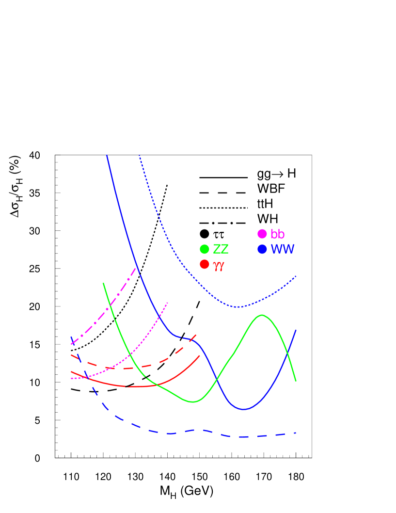
Figure 2: Relative accuracies on the measurement of the cross section of a scalar SM-like Higgs boson in the production+decay channels listed in Table 3. All channels have been rescaled to a total integrated luminosity of 200 fb^-1 (100 fb^-1 per detector), except $pp\to t\bar{t}H,\,H\to WW$ and $q\bar{q}\to WH,\,H\to b\bar{b}$ for which we use 300 fb^-1 [18, 19], and $gg\to H,\,H\to WW$ that was studied for 30 fb^-1 [5] (see text).

By looking at Table 3 and Fig. 2, it seems natural to divide the mass range of an intermediate mass scalar Higgs boson into two main regions, corresponding to $M_{H}\!\leq\!140$ GeV and $140\!<\!M_{H}\!\leq\!180$ GeV. All the existing studies belong to one of these two main mass regions. In particular, in the lower mass region, for $M_{H}\!\leq\!140$ GeV, we consider the following channels:

$$gg\rightarrow H\,\,\,\mbox{with}\,\,\,H\rightarrow\gamma\gamma\,\,\,,$$ (3)

$$qq\rightarrow qqH\,\,\,\mbox{with}\,\,\,H\rightarrow\gamma\gamma,\,\tau\tau,\,WW\,\,\,,$$

$$q\bar{q},gg\rightarrow t\bar{t}H\,\,\,\mbox{with}\,\,\,H\rightarrow b\bar{b},\tau\tau\,\,\,,$$

while in the higher mass region, for $140\!<\!M_{H}\!\leq\!180$ GeV we consider the following channels:

$$gg\rightarrow H\,\,\,\mbox{with}\,\,\,H\rightarrow ZZ,\,WW\,\,\,,$$ (4)

$$qq\rightarrow qqH\,\,\,\mbox{with}\,\,\,h\rightarrow WW\,\,\,.$$

No other convenient choice seems possible at the moment. Since we would like to work with a uniform integrated luminosity of 200 fb^-1 for all channels (100 fb^-1 per detector), we decide not to use $gg\to H,\,H\to WW$ for $M_{H}\!\leq\!140$ GeV, since the corresponding accuracies summarized in Table 3 have been obtained using an integrated luminosity of 30 fb^-1 and are therefore pretty poor in the lower mass region. Rescaling these numbers to a much higher luminosity is debatable and we prefer not to base our analysis on that. On the other hand, we rescale the results obtained for $pp\to t\bar{t}H,\,H\to b\bar{b}$ from 30 fb^-1 [17] to 100 fb^-1, since the nature of the signal over background shape justifies that. To account for both detectors, many results are then rescaled from 100 fb^-1 to 200 fb^-1, and this is clearly adequate.

We also note that we could consider $q\bar{q}\to HW,\,H\to b\bar{b}$ instead of $pp\to t\bar{t}H,\,H\to b\bar{b}$. However this does not seem convenient since, for equal luminosity, the $pp\to t\bar{t}H,\,H\to b\bar{b}$ channel can be measured with better accuracy and, together with $pp\to t\bar{t}H,\,H\to\tau^{+}\tau^{-}$, allows for a model independent measurement of $y_{b}/y_{\tau}$. Of course, in a very high luminosity scenario both channels should be combined in order to obtain better accuracies. We note that for $M_{H}\!>\!140$ GeV there is no channel that can provide a handle on $\Gamma_{b}$. Both $pp\to t\bar{t}H,\,H\to b\bar{b}$ and $q\bar{q}\to WH,\,H\to b\bar{b}$ can possibly be used up to 135-140 GeV, just to cover the entire spectrum of a light MSSM scalar Higgs boson, but not above 140 GeV. In fact, for the purpose of our study, we have extrapolated the existing analysis of $pp\to t\bar{t}H,\,H\to b\bar{b}$ [17] from $M_{H}\!=\!130$ GeV up to $M_{H}\!=\!140$ GeV, for the only purpose of covering the entire MSSM light scalar Higgs boson mass range. For higher masses, the determination of $\Gamma_{b}$ will remain a problem at hadron colliders. On the other hand, for the mass region $M_{H}\!\leq\!140$ GeV, certainly the most interesting one for the scenario we address in this paper, we can use all channels listed in Eq. (3) and we will see how having the extra possibility of measuring $pp\to t\bar{t}H,\,H\to\tau^{+}\tau^{-}$ is indeed crucial.

We start therefore by discussing the most interesting case of a Higgs boson with mass $M_{H}\!\leq\!140$ GeV. This will be indeed the main focus of our analysis. To be consistent with the picture developed up to here, we assume that the width of the Higgs boson is mainly saturated by the decays into $b\bar{b}$, $\tau^{+}\tau^{-}$, $W^{+}W^{-}$, $ZZ$, $gg$, and $\gamma\gamma$. By using the set of measurements in Eq. (3), we can then solve a system of equations of the form given in Eq. (2), one for each channel in Eq. (3). The solution returns the values of the individual rates $\Gamma_{t}$, $\Gamma_{b}$, $\Gamma_{\tau}$, $\Gamma_{w}$, $\Gamma_{g}$, and $\Gamma_{\gamma}$ as functions of the observables $Z^{(i)}_{j}$ and the total rate $\Gamma$. The individual $\Gamma_{i}$ turn out to be:

$$\Gamma_{t} = \frac{Z^{(t)}_{\tau}\sqrt{Z^{(w)}_{w}}}{Z^{(w)}_{\tau}}\sqrt{\Gamma}\,\,\,,$$ (5)

$$\Gamma_{b} = \frac{Z^{(t)}_{b}Z^{(w)}_{\tau}}{Z^{(t)}_{\tau}\sqrt{Z^{(w)}_{w}}}\sqrt{\Gamma}\,\,\,,$$

$$\Gamma_{\tau} = \frac{Z^{(w)}_{\tau}}{\sqrt{Z^{(w)}_{w}}}\sqrt{\Gamma}\,\,\,,$$

$$\Gamma_{w} = \sqrt{Z^{(w)}_{w}}\sqrt{\Gamma}\,\,\,,$$

$$\Gamma_{\gamma} = \frac{Z^{(w)}_{\gamma}}{\sqrt{Z^{(w)}_{w}}}\sqrt{\Gamma}\,\,\,,$$

$$\Gamma_{g} = \frac{Z^{(g)}_{\gamma}\sqrt{Z^{(w)}_{w}}}{Z^{(w)}_{\gamma}}\sqrt{\Gamma}\,\,\,,$$

while the total width $\Gamma$ follows from the assumption that $\Gamma=\Gamma_{b}+\Gamma_{\tau}+\Gamma_{w}+\Gamma_{z}+\Gamma_{g}+\Gamma_{\gamma}$:

$$\sqrt{\Gamma}=\frac{1}{\sqrt{Z^{(w)}_{w}}}\left[Z^{(w)}_{\tau}\left(1+\frac{Z^{(t)}_{b}}{Z^{(t)}_{\tau}}\right)+Z^{(w)}_{w}\left(1+z_{SM}\right)+\frac{Z^{(w)}_{w}Z^{(g)}_{\gamma}}{Z^{(w)}_{\gamma}}+Z^{(w)}_{\gamma}\right]\,\,\,.$$ (6)

Furthermore, we note that we can express the decay rates for $H\to gg$ and $H\to\gamma\gamma$ as the linear combination of terms due to the SM particles that contribute in the loop, plus an extra term that accounts for new physics heavy degrees of freedom. In other words we can write $\Gamma_{g}$ and $\Gamma_{\gamma}$ as

$$\Gamma_{g} \simeq A_{t}^{(g)}\Gamma_{t}+A_{b}^{(g)}\Gamma_{b}+A_{tb}^{(g)}\sqrt{\Gamma_{t}\Gamma_{b}}+\delta_{g}$$ (7)

$$\Gamma_{\gamma} \simeq A_{t}^{(\gamma)}\Gamma_{t}+A_{w}^{(\gamma)}\Gamma_{w}+A_{tw}^{(\gamma)}\sqrt{\Gamma_{t}\Gamma_{w}}+\delta_{\gamma}$$

where we have neglected all the contributions from SM particles that are below the level of accuracy expected on the measurement of $\Gamma_{g}$ and $\Gamma_{\gamma}$ (20-30%), while we have indicated by $\delta_{g}$ and $\delta_{\gamma}$ the unknown loop contributions from new physics. Since we have factored the Higgs couplings square into the corresponding $\Gamma_{i}$’s, we note that the coefficients $A_{t}^{(g,\gamma)}$, $A_{b}^{(g)}$, $A_{tb}^{(g)}$, $A_{w}^{(\gamma)}$, and $A_{tw}^{(\gamma)}$ only depend on $M_{H}$ and on the mass of the SM particle in the loop. They represent the explicit contribution of the top quark, the bottom quark, and the $W$ boson to the $H\to gg$ or $H\to\gamma\gamma$ loop, and can be taken from the corresponding SM calculations [42]. Using the results in Eqs. (5) and (6), the expressions of $\delta_{g}$ and $\delta_{\gamma}$ follow from Eq. (7).

Table 4: Relative accuracy (%) for the total width $\Gamma$ and for the individual $\Gamma_{i}$ obtained in the model-independent scenario (MI) as well as in the scenario with $\Gamma_{b}/\Gamma_{\tau}\!=y_{SM}$ (BT) at the LHC with 200 fb^-1 total integrated luminosity (100 fb^-1 per detector). These values include the systematic theoretical errors.

$M_{H}$ (GeV)		$\Gamma$	$\Gamma_{t}$	$\Gamma_{b}$	$\Gamma_{\tau}$	$\Gamma_{w}$	$\Gamma_{g}$	$\Gamma_{\gamma}$
110	MI	42.6	12.5	47.5	30.4	20.4	35.5	28.5
	BT	25.2	14.9	25.2	25.2	11.0	31.0	22.7
120	MI	38.6	12.7	46.5	26.0	19.3	33.7	23.6
	BT	19.4	15.7	19.9	19.9	9.6	29.3	16.7
130	MI	36.0	16.0	50.8	24.6	18.2	32.7	22.0
	BT	15.6	18.6	18.6	18.6	8.2	28.4	14.9
140	MI	32.8	27.7	62.9	24.8	16.8	32.4	21.3
	BT	12.1	25.1	19.6	19.6	7.0	28.6	14.8

We first determine the relative accuracy on the width, and then use it to calculate the relative accuracy on the individual rates $\Gamma_{i}$. The uncertainty on $\Gamma$, and therefore on the individual rates $\Gamma_{i}$, is a complicated function of the uncertainties on the single experimental channels, that takes into account all theoretical correlations and relies on the assumption that the single Higgs branching ratios have a magnitude comparable to the SM Higgs. In principle, experimental systematics and correlations should also be taken into account, but this information is not yet available. The individual production cross sections are also affected by some theoretical uncertainties, mainly due to higher order radiative corrections. This can be estimated from existing calculations in terms of the residual renormalization and factorization scale dependence, and can be accounted for by adding a systematic error to the corresponding accuracies in Table 3. At the moment $gg\to H$ [43] is affected by the largest theoretical uncertainty, of the order of 15%, while the theoretical uncertainties on $pp\to t\bar{t}H$ and $qq\to qqH$ are of the order of $6\%$ [35, 44, 45] and below $5\%$ [46] respectively. To compare with the analysis done for the $\Gamma_{b}/\Gamma_{\tau}=y_{SM}$ case in Ref. [20], we assume the same conservative theoretical uncertainties of 20% for $gg\to H$, of 10% for $pp\to t\bar{t}H$, and of 5% for $qq\to qqH$. Moreover, when comparing with the $\Gamma_{b}/\Gamma_{\tau}=y_{SM}$ case, we will assume an error on $y_{SM}$ of 7%, due to the uncertainty on the $b$ quark mass.

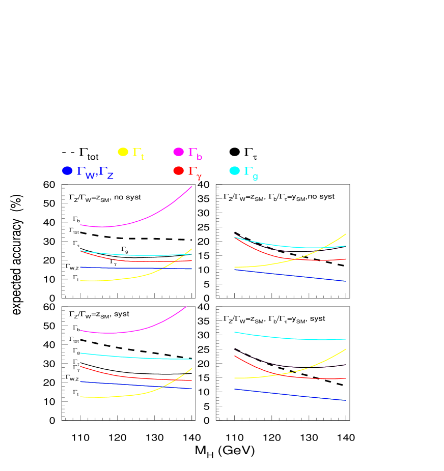
Figure 3: Relative accuracy (%) on the individual rates $\Gamma_{i}$ expected in the model-independent scenario as well as in a scenario with $\Gamma_{b}/\Gamma_{\tau}$ fixed to its SM value, at the LHC with $\sqrt{s}\!=\!14$ TeV. A total integrated luminosity of 200 fb^-1 (100 fb^-1 per detector) is assumed. The upper plots show the accuracies obtained without including any theoretical systematic error, while the lower plots show the same accuracies when a systematic theoretical error of $20\%$ for the $gg\to H$ channel, of $5\%$ for the $qq\to qqH$, and of $10\%$ for $pp\to t\bar{t}H$ channel are included.

Our results for the accuracy on the individual $\Gamma_{i}$ are reported in Table 4, for Higgs masses $M_{H}\!=\!110-140$ GeV, and are illustrated in Fig. 3, both in the case when the systematic theoretical errors discussed above are included and when they are not. We prefer to present both results since some theoretical predictions may be improved in the future, and the accuracies obtained using the present systematic theoretical errors can be treated as upper bounds in future analyses. In the same figure we also show for comparison the accuracies that we obtain by following the same approach outlined above, but fixing the ratio $\Gamma_{b}/\Gamma_{\tau}\!=\!y_{SM}$, as done in Ref. [5, 20]. In this case, the accuracies obtained on the individual $\Gamma_{i}$ by including the theoretical uncertainties discussed in this Section show very good agreement with the results presented in Ref. [20, 21, 22].

As expected, by removing some model dependent assumptions the uncertainty on the single $\Gamma_{i}$ does not generally improve. It is however interesting to note that, due to the interplay between $Z_{b}^{(t)}$ and $Z_{\tau}^{(t)}$ in the error propagation analysis, the accuracy on $\Gamma_{t}$ is reduced with respect to the model-dependent case, and is now definitely in the $10-20\%$ range, even after all theoretical uncertainties has been taken into account. It is also useful to remember that the actual error on the couplings is half the error on the corresponding $\Gamma_{i}$, and therefore, the overall result of the model independent analysis is very encouraging, with accuracies on all couplings between 7% and 25%. Most of all, however, we would like to stress the impact of having included the $pp\to t\bar{t}H,\,H\to\tau^{+}\tau^{-}$ channel with two main considerations. First of all, we can now determine in a completely model independent way ratios of couplings like

$$\frac{\Gamma_{b}}{\Gamma_{\tau}}=\frac{Z^{(t)}_{b}}{Z^{(t)}_{\tau}}\,\,\,\,\,\mbox{and}\,\,\,\,\,\frac{\Gamma_{t}}{\Gamma_{g}}=\frac{Z^{(t)}_{\tau}Z^{(w)}_{\gamma}}{Z^{(w)}_{\tau}Z^{(g)}_{\gamma}}\,\,\,,$$ (8)

with accuracies of the order of 20-30%, as illustrated in Fig. 4. The only residual model dependence in the determination of the individual $Z^{(i)}_{j}$ is in the assumption that the relation between $WWH$ and $ZZH$ weak boson fusion in $qq\to qqH$ is SM-like. However, we note that both ratios in Eq. (8) do not actually depend on such assumption. In fact, only $\Gamma_{t}/\Gamma_{g}$ depends on $Z^{(w)}_{j}$ observables, but the model dependence in assuming $\Gamma_{z}/\Gamma_{w}\!=\!z_{SM}$ cancels between numerator and denominator.

Furthermore, we note that, by adding the $pp\to Ht\bar{t},\,H\to\tau^{+}\tau^{-}$ channel, we provide the possibility of testing the $\Gamma_{z}/\Gamma_{w}\!=\!z_{SM}$ universality assumption even for $M_{H}\!<\!140$ GeV (!) by comparing the two ratios

$$\frac{Z^{(wH)}_{b}}{Z^{(t)}_{b}}\,\,\,\,\,\,\mbox{and}\,\,\,\,\,\,\frac{Z^{(w)}_{\tau}}{Z^{(t)}_{\tau}}\,\,\,,$$ (9)

at high luminosity of the order of 300 fb^-1. Indeed, while the first ratio is always proportional to $\Gamma_{w}/\Gamma_{t}$, the second ratio is proportional to a combination of $\Gamma_{w}/\Gamma_{t}$ and $\Gamma_{z}/\Gamma_{t}$. The comparison between the two ratios can therefore test the assumption that $\Gamma_{z}/\Gamma_{w}\!=\!z_{SM}$. Using the accuracies listed in Table 3, both ratios in Eq. (9) can be measured at the 20-30% level depending on the value of $M_{H}$.

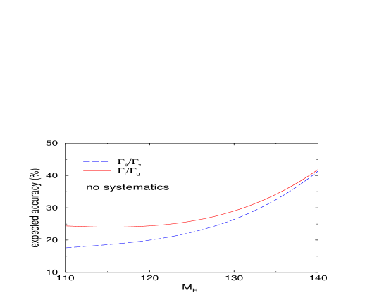
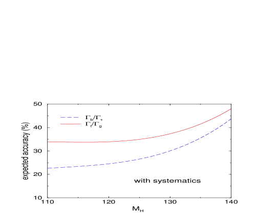
Figure 4: Relative accuracy (%) on the measurement of the ratios $\Gamma_{b}/\Gamma_{\tau}$ and $\Gamma_{t}/\Gamma_{g}$ without (top) and with (bottom) systematic theoretical errors.

Finally, we have studied the accuracy with which $\delta_{g}$ and $\delta_{\gamma}$ can be determined. We summarize our results in Fig. 4 where we plot the expected accuracy for different values of $\delta_{g}/\Gamma_{g}$ and $\delta_{\gamma}/\Gamma_{\gamma}$, and $M_{H}\!=\!120$ GeV. According to the definition in Eq. (7), $\delta_{g}$ and $\delta_{\gamma}$ represent contributions to the $Hgg$ and $H\gamma\gamma$ vertices that are not already accounted for in deviations of the Higgs couplings to the SM degrees of freedom. Therefore they account for loop effects from non-SM heavy degrees of freedom that do not affect the Higgs width directly. It is interesting to note from Fig. 5 that only deviations of the order of 50% or bigger will be measurable with sufficient accuracy. The curves plotted in Fig. 5 are obtained by allowing extra large $\delta_{g}$ or $\delta_{\gamma}$ contributions in either $\Gamma_{g}$ or $\Gamma_{\gamma}$, i.e. not in both at the same time. Therefore this plot contains some model dependence, and has to be taken just as an indication of the fact that it will be hard to measure small purely loop effects at the LHC through $\Gamma_{g}$ and $\Gamma_{\gamma}$.

We conclude by examining the mass region $140\!\leq\!M_{H}\!\leq\!180$ GeV, where we consider the channels listed in Eq. (4). Unfortunately, unless a very exotic Higgs boson is discovered, case that is not considered in this analysis, no model independent way to determine the couplings of a scalar Higgs to both SM fermions and gauge bosons can be developed. In fact, none of the channels listed in Eq. (4) will allow a measurement of the scalar Higgs boson couplings to the $\tau$ lepton or to the bottom quark. The decays into the SM gauge bosons dominate and, as mentioned before, this offers the important possibility to precisely test the $\Gamma_{z}/\Gamma_{w}\!=\!z_{SM}$ assumption at the 20-30% level [5, 20]. Moreover, since $pp\to t\bar{t}H,\,H\to WW$ becomes available, the ratio $\Gamma_{t}/\Gamma_{g}$ can be tested in a model independent way through a measurement of $Z^{(t)}_{w}/Z^{(g)}_{w}$, although this will require luminosities of the order of 300 fb^-1 for the measurement of $Z^{(t)}_{w}$ [18]. Since the $pp\to t\bar{t}H,\,H\to\tau^{+}\tau^{-}$ channel that we have studied in this paper cannot be measured with good accuracy for $M_{H}\!>\!140$ GeV, in this mass region our analysis follows the pattern of existing studies [5, 20, 18] to which we refer for more details.

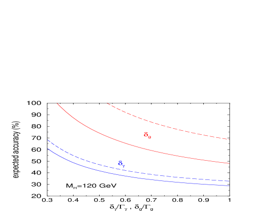
Figure 5: Relative accuracies (%) for $\delta_{g}$ and $\delta_{\gamma}$ obtained in the model-independent scenario, for a scalar Higgs boson with $M_{H}\!=\!120$ GeV, at the LHC with $\sqrt{s}\!=\!14$ TeV. We illustrate both the case in which systematic theoretical errors have been (dashed) and have not been (solid) included. A total integrated luminosity of 200 fb^-1 (100 fb^-1 per detector) is assumed.

4 Conclusions

In this paper we have studied the potential of the LHC to observe a relatively light scalar Higgs boson in the $pp\to t\bar{t}H,\,H\to\tau^{+}\tau^{-}$ process at $\sqrt{s}\!=\!14$ TeV. The study has been mainly done at the parton level, but taking into account detector energy resolution and with the correct simulation of $\tau$-leptons decays. Following the strategy outlined in Section 2, we have shown that for 100 fb^-1 of total integrated luminosity one has 34-8 signal events for $M_{H}\!=\!110-140$ GeV respectively, against about 12 background events.

We have shown that one can use the $pp\to t\bar{t}H,\,H\to\tau^{+}\tau^{-}$ process to measure the $y_{t}\times y_{\tau}$ product of Yukawa couplings. This is a crucial point, since the addition of the $pp\to t\bar{t}H,\,H\to\tau^{+}\tau^{-}$ channel to other already studied Higgs production channels allows to measure the $y_{\tau}$ and $y_{b}$ Yukawa couplings independently and removes the assumption of $y_{b}/y_{\tau}$ universality used in all previous studies. This allows to be sensitive to non-trivial radiative corrections breaking the $y_{b}/y_{\tau}$ universality in models of new physics beyond the SM, notably Supersymmetric models.

For the case of a light scalar Higgs boson, with mass $M_{H}\!\leq\!140$ GeV, we have shown how to derive the accuracies on the measurement of the width and of the individual $y_{t}$, $y_{b}$, $y_{\tau}$, $y_{w}$, $y_{g}$, and $y_{\gamma}$ couplings to SM fermions and gauge bosons. As an example, we have presented the numerical values of these accuracies for a SM-like scenario. Results are encouraging, even when all known systematics are taken into account. Accuracies of the order of 10-20% are expected for most couplings. In this scenario, the ratios of $y_{b}/y_{\tau}$ and $y_{t}/y_{g}$ can be measured in a model independent way, with accuracies that also fall in the 15-20% range. In addition, adding $pp\to Ht\bar{t},\,H\to\tau^{+}\tau^{-}$ provides the possibility of testing the $y_{z}/y_{w}$ universality for Higgs boson masses $M_{H}\!<\!140$ GeV.

We have also investigated the sensitivity to non SM particles contributing to the $Hgg$ or $H\gamma\gamma$ loop-induced vertices, and determined that only very large deviations, of the order of 50% or more, will be measured with sufficient accuracy.

Our final results, presented in Table 4 and illustrated in Figs. 3-5, show that a study of the $pp\to t\bar{t}H,\,H\to\tau^{+}\tau^{-}$ process allows us to make an important step towards a model independent measurement of the couplings of a light scalar Higgs boson at the LHC.

- [1] The LEP Higgs Working Group, Search for the Standard Model Higgs Boson at LEP, LHWG/2001-03, July 2001.
- [2] The LEP Higgs Working Group, Searches for the neutral Higgs Bosons of the MSSM: preliminary combined results using LEP data collected at energies up to 209 GeV, LHWG/2001-04, July 2001.
- [3] The LEP EW Working Group, A combination of preliminary electroweak measurements and constraints on the Standard Model, LEPEWWG/2002-01, May 2002.
- [4] S. Heinemeyer, W. Hollik, and G. Weiglein, The masses of the neutral CP-even higgs bosons in the MSSM: Accurate analysis at the two-loop level, Eur. Phys. J. C9 (1999) 343–366, [arXiv:hep-ph/9812472].
- [5] D. Zeppenfeld, R. Kinnunen, A. Nikitenko, and E. Richter-Was, Measuring Higgs boson couplings at the LHC, Phys. Rev. D62 (2000) 013009, [http://arXiv.org/abs/hep-ph/0002036].
- [6] ATLAS collaboration, Tech. Rep. CERN/LHCC/99-15, CERN, 1999.
- [7] CMS collaboration, Tech. Rep. CERN/LHCC/94-38, CERN, 1994.
- [8] D. Denegri et. al., Summary of the CMS discovery potential for the MSSM SUSY Higgses, http://arXiv.org/abs/hep-ph/0112045.
- [9] D. Rainwater and D. Zeppenfeld, Searching for in weak boson fusion at the LHC, JHEP 12 (1997) 005, [http://arXiv.org/abs/hep-ph/9712271].
- [10] D. L. Rainwater, Intermediate-mass Higgs searches in weak boson fusion, http://arXiv.org/abs/hep-ph/9908378.
- [11] D. Rainwater, D. Zeppenfeld, and K. Hagiwara, Searching for in weak boson fusion at the LHC, Phys. Rev. D59 (1999) 014037, [http://arXiv.org/abs/hep-ph/9808468].
- [12] T. Plehn, D. Rainwater, and D. Zeppenfeld, A method for identifying at the CERN LHC, Phys. Rev. D61 (2000) 093005, [http://arXiv.org/abs/hep-ph/9911385].
- [13] D. Rainwater and D. Zeppenfeld, Observing in weak boson fusion with dual forward jet tagging at the CERN LHC, Phys. Rev. D60 (1999) 113004, [http://arXiv.org/abs/hep-ph/9906218].
- [14] N. Kauer, T. Plehn, D. Rainwater, and D. Zeppenfeld, as the discovery mode for a light Higgs boson, Phys. Lett. B503 (2001) 113–120, [http://arXiv.org/abs/hep-ph/0012351].
- [15] E. Richter-Was and M. Sapinski, Search for the SM and MSSM Higgs boson in the channel, Acta Phys. Polon. B30 (1999) 1001–1040.
- [16] M. Beneke et. al., Top quark physics, http://arXiv.org/abs/hep-ph/0003033.
- [17] V. Drollinger, T. Muller, and D. Denegri, Searching for Higgs bosons in association with top quark pairs in the decay mode, http://arXiv.org/abs/hep-ph/0111312.
- [18] F. Maltoni, D. Rainwater, and S. Willenbrock, Measuring the top-quark Yukawa coupling at hadron colliders via , http://arXiv.org/abs/hep-ph/0202205.
- [19] V. Drollinger, T. Muller, and D. Denegri, Prospects for Higgs boson searches in the channel , http://arXiv.org/abs/hep-ph/0201249.
- [20] D. Zeppenfeld, Higgs couplings at the LHC, http://arXiv.org/abs/hep-ph/0203123.
- [21] D. Cavalli et. al., The Higgs working group: Summary report, http://arXiv.org/abs/hep-ph/0203056.
- [22] Precision Higgs Working Group of Snowmass 2001 Collaboration, J. Conway, K. Desch, J. F. Gunion, S. Mrenna, and D. Zeppenfeld, The precision of Higgs boson measurements and their implications, http://arXiv.org/abs/hep-ph/0203206.
- [23] C. P. Burgess, J. Matias, and M. Pospelov, Higgs or not a Higgs? what to do if you discover a new scalar particle, http://arXiv.org/abs/hep-ph/9912459.
- [24] L. J. Hall, R. Rattazzi, and U. Sarid, The top quark mass in supersymmetric SO(10) unification, Phys. Rev. D50 (1994) 7048–7065, [http://arXiv.org/abs/hep-ph/9306309].
- [25] M. Carena, M. Olechowski, S. Pokorski, and C. E. M. Wagner, Electroweak symmetry breaking and bottom-top Yukawa unification, Nucl. Phys. B426 (1994) 269–300, [http://arXiv.org/abs/hep-ph/9402253].
- [26] M. Carena, D. Garcia, U. Nierste, and C. E. M. Wagner, Effective lagrangian for the interaction in the MSSM and charged Higgs phenomenology, Nucl. Phys. B577 (2000) 88–120, [http://arXiv.org/abs/hep-ph/9912516].
- [27] F. Borzumati, G. R. Farrar, N. Polonsky, and S. Thomas, Soft Yukawa couplings in Supersymmetric theories, Nucl. Phys. B555 (1999) 53–115, [http://arXiv.org/abs/hep-ph/9902443].
- [28] M. Carena, H. E. Haber, H. E. Logan, and S. Mrenna, Distinguishing a MSSM Higgs boson from the SM Higgs boson at a linear collider, Phys. Rev. D65 (2002) 055005, [http://arXiv.org/abs/hep-ph/0106116].
- [29] J. Guasch, W. Hollik, and S. Penaranda, Distinguishing Higgs models in , Phys. Lett. B515 (2001) 367–374, [http://arXiv.org/abs/hep-ph/0106027].
- [30] G. F. Giudice, R. Rattazzi, and J. D. Wells, Graviscalars from higher-dimensional metrics and curvature-Higgs mixing, Nucl. Phys. B595 (2001) 250–276, [http://arXiv.org/abs/hep-ph/0002178].
- [31] J. L. Hewett and T. G. Rizzo, Shifts in the properties of the Higgs boson from radion mixing, http://arXiv.org/abs/hep-ph/0202155.
- [32] G. Cacciapaglia, M. Cirelli, and G. Cristadoro, Gluon fusion production of the Higgs boson in a calculable model with one extra dimension, http://arXiv.org/abs/hep-ph/0111287.
- [33] A. Pukhov et. al., CompHEP: A package for evaluation of Feynman diagrams and integration over multi-particle phase space. User’s manual for version 33, [http://arXiv.org/abs/hep-ph/9908288]
- [34] CTEQ Collaboration, H. L. Lai et. al., Global QCD analysis of parton structure of the nucleon: CTEQ5 parton distributions, Eur. Phys. J. C12 (2000) 375–392, [http://arXiv.org/abs/hep-ph/9903282].
- [35] W. Beenakker et. al., Higgs radiation off top quarks at the Tevatron and the LHC, Phys. Rev. Lett. 87 (2001) 201805, [http://arXiv.org/abs/hep-ph/0107081].
- [36] M. Spira, HIGLU and HDECAY: Programs for Higgs boson production at the LHC and Higgs boson decay widths, Nucl. Instrum. Meth. A389 (1997) 357–360, [http://arXiv.org/abs/hep-ph/9610350].
- [37] A. Djouadi, J. Kalinowski, and M. Spira, HDECAY: A program for Higgs boson decays in the Standard Model and its supersymmetric extension, Comput. Phys. Commun. 108 (1998) 56–74, [http://arXiv.org/abs/hep-ph/9704448].
- [38] A. S. Belyaev, E. E. Boos, and L. V. Dudko, Single top quark at future hadron colliders: Complete signal and background study, Phys. Rev. D59 (1999) 075001, [http://arXiv.org/abs/hep-ph/9806332].
- [39] A. S. Belyaev et. al., CompHEP-PYTHIA interface: Integrated package for the collision events generation based on exact matrix elements, http://arXiv.org/abs/hep-ph/0101232.
- [40] S. Jadach, Z. Was, R. Decker, and J. H. Kuhn, The decay library TAUOLA: Version 2.4, Comput. Phys. Commun. 76 (1993) 361–380.
- [41] B. K. Bullock, K. Hagiwara, and A. D. Martin, polarization and its correlations as a probe of new physics, Nucl. Phys. B395 (1993) 499–533.
- [42] M. Spira, QCD effects in Higgs physics, Fortsch. Phys. 46 (1998) 203–284, [http://arXiv.org/abs/hep-ph/9705337].
- [43] R. V. Harlander and W. B. Kilgore, Next-to-next-to-leading order Higgs production at hadron colliders, http://arXiv.org/abs/hep-ph/0201206.
- [44] L. Reina and S. Dawson, Next-to-leading order results for production at the Tevatron, Phys. Rev. Lett. 87 (2001) 201804, [http://arXiv.org/abs/hep-ph/0107101].
- [45] L. Reina, S. Dawson, and D. Wackeroth, QCD corrections to associated production at the Tevatron, Phys. Rev. D65 (2002) 053017, [http://arXiv.org/abs/hep-ph/0109066].
- [46] T. Han, G. Valencia, and S. Willenbrock, Structure function approach to vector boson scattering in collisions, Phys. Rev. Lett. 69 (1992) 3274–3277, [http://arXiv.org/abs/hep-ph/9206246].