UMN–TH–2103/02

TPI–MINN–02/18

SUSX–TH/02-011

hep-ph/0205269

May 2002

Constraints on the Variations of the Fundamental Couplings

Keith A. Olive^1,2, Maxim Pospelov³, Yong-Zhong Qian²,

Alain Coc⁴, Michel Cassé ^5,6, and Elisabeth Vangioni-Flam⁵

¹Theoretical Physics Institute, School of Physics and Astronomy,
University of Minnesota, Minneapolis, MN 55455, USA

²School of Physics and Astronomy,
University of Minnesota, Minneapolis, MN 55455, USA

⁴CSNSM, IN2P3/CNRS/UPS, Bât 104, 91405 Orsay, FRANCE

⁵IAP, CNRS, 98 bis Bd Arago 75014 Paris, FRANCE

⁶SAp, CEA, Orme des Merisiers, 91191 Gif/Yvette CEDEX, FRANCE

Abstract

We reconsider several current bounds on the variation of the fine-structure constant in models where all gauge and Yukawa couplings vary in an interdependent manner, as would be expected in unified theories. In particular, we re-examine the bounds established by the Oklo reactor from the resonant neutron capture cross-section of ¹⁴⁹Sm. By imposing variations in $\Lambda_{QCD}$ and the quark masses, as dictated by unified theories, the corresponding bound on the variation of the fine-structure constant can be improved by about 2 orders of magnitude in such theories. In addition, we consider possible bounds on variations due to their effect on long lived $\alpha$- and $\beta$-decay isotopes, particularly ¹⁴⁷Sm and ¹⁸⁷Re. We obtain a strong constraint on $\Delta\alpha/\alpha$, comparable to that of Oklo but extending to a higher redshift corresponding to the age of the solar system, from the radioactive life-time of ¹⁸⁷Re derived from meteoritic studies. We also analyze the astrophysical consequences of perturbing the decay $Q$ values on bound state $\beta$-decays operating in the $s$-process.

1 Introduction

The nature of fundamental constants in physics is a long-standing problem. While certain constants can be thought of as merely unit conversions ($c,\hbar$, $k_{B}$, etc.), others such as gauge and Yukawa couplings can be thought of as dynamical variables. Indeed, such is the case in string theory, where the only fundamental parameter is dimensional, namely the string tension. The dimensionless gauge and Yukawa couplings are then set by ratios of the dilaton and moduli field vacuum expectation values to the string tension. Similarly the gravitational coupling (Planck mass) is scaled from the string tension by a modulus vev. Thus until these vevs are fixed, the fundamental coupling constants could vary in time. Of course, it is widely expected that non-perturbative effects will generate a potential for the moduli and fix their vev’s (probable at some high energy scale), the mechanism and scale of this fixing are a subject of much debate. Thus in principle, one can consider variations in the fundamental couplings a logical possibility.

Indeed, a considerable amount of interest in the possibility of time-varying constants has been generated by recent observations of quasar absorption systems. Observations of the energy level splitting between the $S_{1/2}\to P_{3/2}$ and $S_{1/2}\to P_{1/2}$ transitions in several atomic states such as CIV, MgII, and SiIV, suggest a time variation in the fine structure constant by an amount ${\Delta\alpha/\alpha}=(0.72\pm 0.18)\times 10^{-5}$ [2] over a redshift range of 0.5 – 3.5. In addition, there may be preliminary evidence for a variation ${\Delta\mu/\mu}=(5.7\pm 3.8)\times 10^{-5}$ in the ratio of the proton to electron masses $\mu\equiv m_{p}/m_{e}$ [3] for redshifts of $\sim$ 2 – 3.

Starting from the work of Bekenstein [4], there have been a number of attempts to formulate a dynamical model of a variable fine structure constant [5, 6]. These models typically consist of a massless scalar field which has a linear coupling to the $F^{2}$ term of the $U(1)$ gauge field. The coupling of non-relativistic matter to the scalar field induces a cosmological change in the background value of this field which can be interpreted as a change in the effective fine structure constant. Independent of our prejudices (or lack thereof) regarding a fundamental theory, such models are difficult to construct in such a way as to remain consistent with other experimental constraints. For example, the presence of a massless scalar field in the theory leads to the existence of an additional attractive force which does not respect Einstein’s weak universality principle. The extremely accurate checks of the latter [7] lead to a firm bound that confines possible changes of $\alpha$ to the range $\Delta\alpha/\alpha<10^{-10}-10^{-9}$ for $0<z<5$ [4, 8, 6] in the context of the minimal Bekenstein model where a change in the scalar field is triggered by the baryon energy density. It was argued [6] that a significant $O(1)$ coupling between the scalar field and the dark matter energy density is required in order to allow ${\Delta\alpha/\alpha}\sim 10^{-5}$ and remain consistent with equivalence principle constraints [7]. Thus it is natural to expect that in generalized Bekenstein models, not only the fine structure constant but all of the couplings and masses will depend on the expectation value of a light scalar.

In addition, there exist various sensitive experimental checks that coupling constants do not change (See e.g., [9]). Among the most stringent of these is the bound on $|\Delta\alpha/\alpha|$ extracted from the analysis of isotopic abundances from the Oklo phenomenon [10]-[13], a natural nuclear fission reactor that occurred about 1.8 billion years ago. While the Oklo bound $|\Delta\alpha/\alpha|<10^{-7}$ is considerably tighter than the “observed” variation, Oklo occurred at a time period corresponding to a redshift of about 0.14, and it is quite possible that while $\alpha$ varied at higher redshifts, it has not varied recently. That is, there is no reason for the variation to be constant in time. Big bang nucleosynthesis also provides limits on $\Delta\alpha/\alpha$ [14, 15]. Although these limits are weaker, they are valid over significantly longer timescales.

The Bekenstein model and its modifications are introduced in ad hoc manner, and their relation to deeper motivated theoretical models is problematic. A major stumbling point on the path between the theory and phenomenology of a changing $\alpha$ is the masslessness of the modulus that mediates this change [16]. Indeed, to be relevant for the cosmological evolution now or in the recent past, the mass of this scalar has to be comparable or lighter than the Hubble parameter at $z\sim 0-5$, whereas quantum corrections would tend to generate a much larger mass. This is a generic problem for any interacting quintessence-like model that is similar to the cosmological constant problem. Since very little is actually understood about the latter, we do not think that this problem is a sufficient reason to discard phenomenological models of changing $\alpha$. Disregarding the problem of masslessness of the modulus that renormalizes coupling constants, we proceed to analyze phenomenological constraints on a theory with a fixed (modulus-independent) high-energy scale $M_{P}$, unified values for all coupling constants at $M_{P}$, and a single modulus that changes the values of all coupling constants. Such a theory is motivated by a string model with dilaton-dependent coupling constants. One has to keep in mind, however, that the simplest string tree-level values for the couplings of dilaton to matter and $m_{dilaton}=0$ lead to a catastrophic non-universality in the gravitational exchange by this scalar, which violates the current bound by 10 orders of magnitude [6, 17]. One remedy to this problem may be a more complicated form of the dilaton-matter coupling with a universal extremum [17]. Another possibility is that a massless modulus contains a relatively small admixture of the string dilaton, so that all the couplings of this modulus to matter are suppressed to a level consistent with the equivalent principle [7].

The possibility that significantly stronger constraints on the variation of the fine structure constant can be obtained in the context of theories in which the change in a scalar field vev induces a change in the fine structure constant as well as the other gauge and Yukawa couplings was first explored in [15] (see also, [18]). There it was recognized that in any unified theory in which the gauge fields have a common origin, variations in the fine structure constant will be accompanied by similar variations in the other gauge couplings. In other words, variations of the gauge coupling at the unified scale will induce variations in all of the gauge couplings at the low energy scale. Note that even in theories with non-universality at the string scale, there is almost always some relation between the couplings.

It is easy to see that the running of the strong coupling constant has dramatic consequences for the low energy hadronic parameters, including the masses of nucleons [15]. Indeed the masses are determined by the QCD scale, $\Lambda$, which is related to the ultraviolet scale, $M_{UV}$, by dimensional transmutation:

$$\alpha_{s}(M_{UV}^{2})\equiv{g_{s}^{2}(M_{UV}^{2})\over 4\pi}={4\pi\over b_{3}\ln(M_{UV}^{2}/\Lambda^{2})},$$ (1.1)

where $b_{3}$ is a usual renormalization group coefficient that depends on the number of massless degrees of freedom, running in the loop. Clearly, changes in $g_{s}$ will induce (exponentially) large changes in $\Lambda$:

$${\Delta\Lambda\over\Lambda}={2\pi\over 9\alpha_{s}(M_{UV})}{\Delta\alpha_{s}(M_{UV})\over\alpha_{s}(M_{UV})}\gg{\Delta\alpha_{s}(M_{UV})\over\alpha_{s}(M_{UV})},$$ (1.2)

where for illustrative purposes we took the beta function of QCD with three fermions. On the other hand, the electromagnetic coupling $\alpha$ never experiences significant running from $M_{UV}$ to $\Lambda$ and thus $\Delta\Lambda/\Lambda\gg\Delta\alpha/\alpha$. A more elaborate treatment of the renormalization group equations above $M_{Z}$ [19] leads to the result that is in perfect agreement with [15]:

$${\Delta\Lambda\over\Lambda}\simeq 30{\Delta\alpha\over\alpha}.$$ (1.3)

In addition, we expect that not only the gauge couplings will vary, but all Yukawa couplings are expected to vary as well. In [15], the string motivated dependence was found to be

$${\Delta h\over h}={\Delta\alpha_{U}\over\alpha_{U}}$$ (1.4)

where $\alpha_{U}$ is the gauge coupling at the unification scale and $h$ is the Yukawa coupling at the same scale. However in theories in which the electroweak scale is derived by dimensional transmutation, changes in the Yukawa couplings (particularly the top Yukawa) leads to exponentially large changes in the Higgs vev. In such theories, the Higgs expectation value corresponds to the renormalization point and is given qualitatively by

$$v\sim M_{P}\exp(-2\pi c/\alpha_{t})$$ (1.5)

where $c$ is a constant of order 1, and $\alpha_{t}=h_{t}^{2}/4\pi$. Thus small changes in $h_{t}$ will induce large changes in $v$. For $c\sim h_{t}\sim 1$,

$${\Delta v\over v}\sim 80{\Delta\alpha_{U}\over\alpha_{U}}$$ (1.6)

This dependence gets translated into a variation in all low energy particle masses. In short, once we allow $\alpha$ to vary, virtually all masses and couplings are expected to vary as well, typically much more strongly than the variation induced by the Coulomb interaction alone. Unfortunately, it is very hard to make a quantitative prediction for $\Delta v/v$ simply because we do not know exactly how the dimensional transmutation happens in the Higgs sector, and the answer will depend, for example, on such things as the dilaton dependence of the supersymmetry breaking parameters. This uncertainty is characterized in Eq. (1.5) by the parameter $c$. For the purpose of the present discussion it is reasonable to assume that $\Delta v/v$ is comparable but not exactly equal to $\Delta\Lambda/\Lambda$. That is, although they are both $O(10-100)\Delta\alpha/\alpha$, their difference $|\Delta\Lambda/\Lambda-\Delta v/v|$ is of the same order of magnitude which we will take as $\sim 50\Delta\alpha/\alpha$.

In [15], these relations were exploited to derive a strong bound on variations of $\alpha$ during big bang nucleosynthesis. The standard limit [14] of ${\Delta\alpha/\alpha}\mathrel{\raise 1.29167pt\hbox{$<$\kern-7.5pt\lower 4.30554pt\hbox{$\sim$}}}10^{-2}$ is improved by about 2 orders of magnitude to ${\Delta\alpha/\alpha}\mathrel{\raise 1.29167pt\hbox{$<$\kern-7.5pt\lower 4.30554pt\hbox{$\sim$}}}10^{-4}$ as recently confirmed in a numerical calculation [20]. Here, we will consider the effect of these relations on the existing Oklo bounds as well as derive new bounds relating to the long lived $\alpha$- and $\beta$-decaying isotopes, ¹⁴⁷Sm and ¹⁸⁷Re; we will also comment briefly on the influence of changing the fundamental couplings on $s$-process yields.

Before proceeding, we note briefly that in the class of theories we are considering, we would predict that the proton-electron mass ratio is also affected. For example, we would expect that

$${\Delta\mu\over\mu}\sim{\Delta\Lambda\over\Lambda}-{\Delta v\over v}$$ (1.7)

From Eqs. (1.3) and (1.6), we estimate that ${\Delta\mu/\mu}\sim 3\times 10^{-4}$, based on the reported claim of a variation in $\alpha$ [2] and is somewhat larger than that reported in [3]. For related discussions see [21].

2 The Oklo Bound Revisited

Approximately two billion years ago, a natural fission reactor was operating in the Oklo uranium mine in Gabon. Shlyakhter [10] argued that a strong limit on the time variation of $\alpha$ was possible by examining the isotopic ratios of Sm in the Oklo reactor. This suggestion was confirmed by Damour and Dyson [11], who performed a detailed analysis of the isotopic ratios and the effect that varying $\alpha$ would have on the resonant neutron capture cross section of Sm. Their analysis provided a bound of

$$\left|{\Delta\alpha\over\alpha}\right|\mathrel{\raise 1.29167pt\hbox{$<$\kern-7.5pt\lower 4.30554pt\hbox{$\sim$}}}10^{-7}$$ (2.8)

The bound was derived primarily by calculating the shift in the resonance energy, $E_{r}\simeq 0.0973$ eV, of the Sm neutron capture cross section which is induced by a variation in the Coulomb contribution. While a full analytical understanding of the energy levels of heavy nuclei is not available, it is nevertheless possible to obtain an estimate of the size of an energy shift if the fundamental parameters of the theory are varied. In particular, it is possible to identify the over-riding scale dependence of the terms which determine the binding energy of the heavy nuclei. We perform this estimate in the context of the Fermi gas model. We will argue that the Oklo data can provide a sufficiently strong bound on the variation of $m_{q}$ and $\Lambda$, or more precisely, on the variation of $m_{q}/\Lambda$.

We begin by considering the semi-empirical formula for the binding energy $B(A,Z)$ of a spherical nucleus with mass number $A$ and atomic number $Z$ [22]:

$$B(A,Z)=C_{V}A-C_{S}A^{2/3}-a_{C}Z^{2}A^{-1/3}+\delta(A,Z)a_{\rm pair}A^{-\epsilon}+C_{d}Z^{2}A^{-1}+\Delta_{\rm shell}(A,Z),$$ (2.9)

where the first three terms on right-hand side represent the volume, surface, and Coulomb contributions, respectively, and the last three terms represent corrections due to pairing, surface diffusiveness, and shell structure. The corrections due to asymmetry between neutrons and protons are included in $C_{V}$ and $C_{S}$. The coefficients in Eq. (2.9) are given by

$$C_{V} = a_{V}\left[1-\kappa\left({A-2Z\over A}\right)^{2}\right],$$ (2.10)

$$C_{S} = a_{S}\left[1-\kappa\left({A-2Z\over A}\right)^{2}\right],$$ (2.11)

$$a_{C} = {3\over 5}{e^{2}\over r_{0}},$$ (2.12)

$$C_{d} = {\pi^{2}\over 2}\left({a_{0}\over r_{0}}\right)^{2}{e^{2}\over r_{0}}.$$ (2.13)

Numerical values for the pertinent quantities are $a_{V}=15.68$ MeV, $a_{S}=18.56$ MeV, $\kappa=1.79$, $a_{C}=0.717$ MeV, $a_{0}=0.546$ fm, $r_{0}=1.205$ fm, $a_{\rm pair}=11$ MeV, $\epsilon=0.5$, and

$$\delta(A,Z)=\left\{\begin{array}[]{rl}1&\mbox{for even-$A$ even-$Z$},\\ 0&\mbox{for odd-$A$},\\ -1&\mbox{for even-$A$ odd-$Z$}.\end{array}\right.$$ (2.14)

The shell structure coefficients are discussed below.

The Coulomb contribution has a simple interpretation as the electromagnetic energy stored in a uniformly charged sphere of total charge $Ze$ and radius $r_{0}A^{-1/3}$. The volume and surface contributions can be rewritten as:

$$C_{V}A-C_{S}A^{2/3}=-(\langle T\rangle+\langle V\rangle),$$ (2.15)

where $T$ and $V$ represent the kinetic and potential energy, respectively, of the nucleons. Based on the Fermi gas model and considerations of nucleon-nucleon interaction potential [22],

$$\langle T\rangle = T_{0}\left[1+{5\over 9}\left({A-2Z\over A}\right)^{2}\right]\left(1-{f_{S}\over A^{1/3}}\right)A,$$ (2.16)

$$\langle V\rangle = \left[V_{V}+V_{\rm sym}\left({A-2Z\over A}\right)^{2}\right]\left(1-{f_{S}\over A^{1/3}}\right)A,$$ (2.17)

where

$$T_{0}={3\over 10}{k_{F}^{2}\over M}\propto{1\over Mr_{0}^{2}}$$ (2.18)

is the zeroth-order contribution to the total kinetic energy and the terms with the coefficient $f_{S}$ represent surface correction. For a Fermi momentum $k_{F}=1.36$ fm^-1, $T_{0}=23.01$ MeV, and the other quantities can be obtained as $V_{V}=-38.69$ MeV, $V_{\rm sym}=15.29$ MeV, and $f_{S}=1.184$.

Now consider the reaction

$${}^{149}{\rm Sm}+n\to^{150}{\rm Sm}+\gamma.$$ (2.19)

The $Q$-value of the reaction is

$$Q = B(150,62)-B(149,62)$$ (2.20)

$$= -0.987T_{0}-0.851V_{V}-0.245V_{\rm sym}+1.615a_{C}+8.16\times 10^{-2}a_{\rm pair}-0.172C_{d}$$

$$+\Delta_{\rm shell}(150,62)-\Delta_{\rm shell}(149,62),$$

where the numerical values for all the terms except for the last two on the right-hand side are $-22.71$, 32.93, $-3.75$, 1.16, 0.90, $-0.21$ MeV, respectively. Comparing the $Q$-value calculated above with the experimental value of 7.99 MeV gives an estimate of $\Delta_{\rm shell}(150,62)-\Delta_{\rm shell}(149,62)=0.33$ MeV. Clearly, changes in $T_{0}$ and $V_{V}$ produce the largest effects on the $Q$-value. Thus not only will our limit be strengthened (relative to the purely electromagnetic bound [11]) due to the strong interaction, but also due to the enhanced sensitivity of the binding energy relative to the Coulomb term alone.

Since we are lacking a complete analytical theory for the origin of the terms entering into Eq. (2.9), it will be sufficient to concentrate on the dominant kinetic and potential terms. Even in this simplified formalism, it is not possible to account for the exact scaling of the dimensionful terms $T_{0}$, $V_{V}$ and $V_{\rm sym}$. However, we can identify a certain degree of required scaling, and it is quite clear that an exact cancellation of such a scaling is extremely unlikely. Furthermore, the resonant cross-section proceeds through an excited state of ¹⁵⁰Sm, which happens to lie very close to the Q value given in Eq. (2.20). Thus the quantity of interest is,

$$E_{r}=Q-E^{*}=0.0973{\rm eV}$$ (2.21)

where $E^{*}$ is the energy of the excited state of ¹⁵⁰Sm. Unfortunately, we expect that variations in the fundamental couplings also lead to changes in $E^{*}$. The previous bound on $\alpha$ was based on the presumption that taking into account the variation of $E^{*}$ with $\alpha$ only strengthens the bound, so that a conservative bound on $\Delta\alpha$ can be traced directly to $\Delta Q$. Here we will have to rely on the probability that it is also highly unlikely that both $Q$ and $E^{*}$ depend on all of the fundamental parameters in exactly the same way. We return to this point below.

Before we derive our bound on possible variations of the gauge couplings it will be useful to first use Eq. (2.20) to derive the bound on $\alpha$ along the lines of [11]. If we ignore all of the unification arguments given in the previous section, then the only clearly identifiable piece with the electromagnetic coupling in Eq. (2.20) is the Coulomb term. Damour and Dyson (1996) [11] derived the bound

$$-0.12{\rm eV}<\Delta(Q-E^{*})=\Delta Q<0.09{\rm eV}$$ (2.22)

where

$$\Delta Q\equiv Q^{\rm Oklo}-Q^{\rm now}$$ (2.23)

For our purposes it will be sufficient to consider the limit $|\Delta Q|<0.1$ eV. The Coulomb term in Eq. (2.20) is simply

$$1.6a_{C}\simeq 1.16{\rm MeV}\,\left({\alpha\over\alpha_{0}}\right)$$ (2.24)

where $\alpha_{0}$ is the present value of the fine structure constant. Thus

$$\Delta Q=1.16{\rm MeV}\,\left({\Delta\alpha\over\alpha}\right)$$ (2.25)

We can therefore immediately derive the limit

$$\left|{\Delta\alpha\over\alpha}\right|\mathrel{\raise 1.29167pt\hbox{$<$\kern-7.5pt\lower 4.30554pt\hbox{$\sim$}}}10^{-7}$$ (2.26)

in good agreement with Damour and Dyson.

We next attempt to use the same procedure to derive the limit on the gauge coupling when the unification argument of the previous section is included. We first note that if we simply associate all dimensionful quantities as originating from $\Lambda_{QCD}$, no significant limit is possible. In such a naive approach, one would argue that the masses of the light quarks can be neglected, and all hadronic parameters such as $m_{N}$ and the strength of the nucleon-nucleon potential scale linearly with $\Lambda$. It is clear, though, that in this limit there is no sizable effect on the position of the resonance, since

$${\Delta E_{r}}\sim\Delta(Q-E^{*})\sim{(Q-E^{*})\over\Lambda}\Delta\Lambda$$ (2.27)

and hence $\Delta E_{r}/E_{r}\sim\Delta\Lambda/\Lambda$. Since the constraint on variation in $E_{r}$ is only $O(1)$ (cf. Eq. (2.22)), one is simply left with $\Delta\Lambda/\Lambda<O(1)$. This point has been repeatedly stressed in the literature. For the most recent discussion, see, e.g. Ref. [23].

There are two generic problems that prevent a rigorous analysis of $\Delta E_{r}$ as a function of $m_{q}/\Lambda$. The first problem lies in fact on the interface of the perturbative QCD description and the description in terms of hadrons. In short, we do not know the exact dependence of hadronic masses and coupling constants on $\Lambda$ and light quark masses. The second problem concerns modeling nuclear forces in terms of the hadronic parameters.

Generically, the mass of a hadron $i$ can be parameterized as

$$m_{i}\simeq const~{}\Lambda\left(1+{\kappa_{i}}\frac{m_{q}}{\Lambda}+O(m_{q}^{2})\right),$$ (2.28)

where $\kappa_{i}$ reflects the dependence on the light quark mass. Clearly, masses of the members of the lightest pseudoscalar octet have a significant dependence on $m_{q}$, and $\kappa_{\pi}\sim 1/2$. On the other hand, heavy hadrons remain massive in the chiral limit which suggests that for nucleons $\kappa_{N}\ll 1$. In practice, $\kappa_{N}$ (Fig 1a) probably varies from 0.1 to 0.2 due in part to a rather large value of the matrix element of $m_{s}\bar{s}s$ over a nucleon state, $\langle N|m_{s}\bar{s}s|N\rangle\sim 100\pm 50$ MeV [24], which is known to admittedly poor accuracy (the combined matrix element over $u$ and $d$ quarks is 45 MeV). Other particles which are important for nuclear dynamics such as vector resonances are expected to have $\kappa_{N}<\kappa_{V}<\kappa_{\pi}$. We note that although a complete analysis of $\Delta m_{i}/\Delta m_{q}$ is certainly lacking (due to the difficulty of the problem), some insight can be gained from QCD sum rule analyses.

Figure 1: The $m_{q}$ dependence of hadronic parameters. (a) illustrates the insertion of $m_{q}\bar{q}q$ into the nucleon line that determines $\kappa_{N}$. (b) is the chiral loop that gives the $m_{q}$ dependence of the nucleon-nucleon interaction.

Recent progress in understanding the chiral dynamics of few nucleon systems is not directly applicable to large nuclei such as Sm (See e.g., [25] and references therein). Instead, one has to resort to a model description of nuclear forces such as contact interactions generated by $t$-channel exchanges of vector and scalar resonances. In this approach, the relevant Lagrangian can be symbolically written as

$${\cal L}=\sum\bar{N}(i\partial_{\mu}\gamma_{\mu}-m_{N})N+\frac{a}{M^{2}}(\bar{N}N)(\bar{N}N)$$ (2.29)

where the sum runs over all relevant isospin and Lorentz structures. The scale $M$ remains finite in the chiral limit, and thus scales approximately linearly with $\Lambda$. It is important to note that single pion exchange, which is the most important source of the nuclear force in the deuteron, plays little if any role in nuclei with large $A$. Nevertheless, one can provide a conservative estimate of the $m_{q}$ dependence of a nucleon-nucleon potential by considering chiral loop corrections to the contact nucleon-nucleon interaction, Fig. 1b. This way one obtains

$$\frac{a}{M^{2}}=\frac{a_{0}}{\Lambda^{2}}+\frac{a_{1}m_{q}}{\Lambda^{3}}+\frac{1}{8\pi^{2}f_{\pi}^{2}}\left(\frac{\langle N|m_{q}\bar{q}q|N\rangle}{f_{\pi}}\right)^{2}\ln\left[\frac{4\pi f_{\pi}}{m_{\eta}}\right]+O(m_{q}^{2}),$$ (2.30)

and $f_{\pi}$ scales linearly with $\Lambda$. In principle, the strength of overall numerical ($\Lambda$ and $m_{q}$ independent) coefficient $a$ can be fit to nuclear data but for the purpose of present discussion, we simply take it to be $O(1)$. Unfortunately, there is no known reliable way of calculating the coefficients $a_{0}$ and $a_{1}$ in front of the zeroth and first order terms of the expansion in $m_{q}$. On the other hand, it is very unlikely that $a_{0}$ and $a_{1}$ would conspire to form exactly the same combination of $\Lambda$ and $m_{q}$ as in $m_{N}$, (2.28). Fortunately, the presence of a chiral logarithm in (2.30) in the $O(m_{q}^{2})$ term and the known absence of such a term in $m_{N}$ ensures that the nucleon mass, $m_{N}$, and the interaction strength, $1/M^{2}$, depend differently on $(m_{q}/\Lambda)$. Thus, to be very conservative, we consider only the variation of the chiral logarithm in (2.29) and use 100 – 200 MeV for the value of $\langle N|m_{q}\bar{q}q|N\rangle$[24], noting that the linear term (of order $m_{q}$) is likely to produce a more stringent bound:

$$\Delta{\cal L}\sim(1-4)\times 10^{-1}{\rm fm}^{2}(\bar{N}N)(\bar{N}N)\frac{\Delta(m_{q}/\Lambda)}{m_{q}/\Lambda}+...$$ (2.31)

From $\Delta{\cal L}$ we obtain the Hamiltonian $\Delta H$ using the mean field approximation:

$$\Delta H=(1-4)\times 10^{-1}{\rm fm}^{2}n_{0}\frac{\Delta(m_{q}/\Lambda)}{m_{q}/\Lambda}\sum_{i}\theta(R-r_{i}),$$ (2.32)

where $R$ is a nuclear radius and $n_{0}$ an average nuclear density inside the nucleus, $n_{0}\simeq 0.17$ fm^-3. The sum runs over all nucleons inside a given nucleus. As discussed above, the change in the position of the resonance comes as the result of the change in the position of the ground state of ¹⁴⁹Sm and the excited state of ¹⁵⁰Sm. In this naive approach, we have neglected all specific origins of the resonant energy found in $Q$ and $E^{*}$. If we then associate $\Delta E_{r}$ with the difference in $\Delta H$ between the relevant states of ¹⁴⁹Sm and ¹⁵⁰Sm, we obtain

$$\frac{|\Delta E_{r}|}{E_{r}}\sim\frac{(1-4)\times 10^{-1}{\rm fm}^{2}n_{0}}{E_{r}}\left|\frac{\Delta(m_{q}/\Lambda)}{m_{q}/\Lambda}\right|\sim(2.5-10)\times 10^{7}\left|\frac{\Delta v}{v}-\frac{\Delta\Lambda}{\Lambda}\right|.$$ (2.33)

Note, that our result (2.33) is about an order of magnitude weaker than the result obtained in [23]. Applying $|\Delta E_{r}/E_{r}|<1$ [11], we arrive at the following bound:

$$\left|\frac{\Delta v}{v}-\frac{\Delta\Lambda}{\Lambda}\right|<(1-4)\times 10^{-8}$$ (2.34)

In the theoretical framework discussed in this paper, the result (2.34) allows us to improve the limits on the variation of the coupling constant by over an order of magnitude compared to Ref. [11]. Indeed, combining eqs. (2.34) and the estimate $|\Delta\Lambda/\Lambda-\Delta v/v|\sim 50\Delta\alpha/\alpha$, one gets

$$\left|\frac{\Delta\alpha}{\alpha}\right|<(2-8)\times 10^{-10}$$ (2.35)

We remind the reader that the range quoted in the limit above is due to the uncertainty in the strange quark contribution to the nucleon mass and corresponds to using 100 – 200 MeV for $\langle N|m_{q}\bar{q}q|N\rangle$.

It is also possible (though it bears its share of uncertainty) to use the expression for $Q$ (2.20) to further strengthen the bound. One should note that the resonance energy, $E_{r}$, is tiny due to a cancellation between $Q$ and $E^{*}$. Both are individually $\approx 8$ MeV. However, the value of $Q$ is also determined by a set of cancellations between the terms in Eq. (2.20) which are of order 20-30 MeV. By once again relying on the improbability that all terms will depend on the fundamental constant in the same way, one can in principle use only the largest term (or terms) in $Q$, which are the potential and kinetic terms.

If we again parameterize our ignorance of exact scalings with $|\Delta\Lambda/\Lambda-\Delta v/v|$, we can expect that

$${\Delta E_{r}\over E_{r}}\sim{\Delta(Q-E^{*})\over E_{r}}\sim{\Delta V\over E_{r}}\sim{V\over E_{r}}\kappa\left|\frac{\Delta v}{v}-\frac{\Delta\Lambda}{\Lambda}\right|<1$$ (2.36)

which leads to

$$\left|\frac{\Delta\alpha}{\alpha}\right|<(1-5)\times 10^{-10}$$ (2.37)

for the range $0.1\mathrel{\raise 1.29167pt\hbox{$<$\kern-7.5pt\lower 4.30554pt\hbox{$\sim$}}}\kappa<0.5$. In Eq. (2.37), we have assumed $V\sim 30$ MeV. This is the most optimistic bound that one can expect from the Oklo data. Recalling, that the Oklo event occurred some 2 Gyr in the past, we would obtain the limit $\dot{\alpha}/\alpha<2.5\times 10^{-19}$ yr^-1.

3 Constraints on the variation of fundamental couplings from long lived $\alpha$- and $\beta$-decay nuclei

Bounds on the variation of the fundamental couplings can also be obtained from our knowledge of the lifetimes of certain long-lived nuclei. In particular, it is possible to use relatively precise meteoritic data to constrain nuclear decay rates back to the time the solar system was formed (about 4.6 Gyr ago). Thus, for the current standard inputs of $\Omega_{m}\simeq 0.35$, $\Omega_{\Lambda}\simeq 0.65$ and $h_{0}=0.71$, we can derive a constraint on possible variations at a redshift $z\simeq 0.45$ which borders the range over which such variations are claimed to be observed ($z$ = 0.5 – 3.5). Note that nuclei with relatively short lifetimes, especially in the case of bound beta-decay (see section 4), could be of astrophysical interest in the context of $s$-process nucleosynthesis [26].

3.1 Nuclear physics

Here, we will concentrate only on the possible influence of variations in the $Q$-value on $\alpha$- and $\beta$-decay lifetimes. As fission processes are less well understood and less sensitive than the other decay processes, we do not consider those isotopes for which fission is the dominant decay mode. On the other hand, $\alpha$- and $\beta$-decay processes are better understood, and our basic constraints can be seen as due to a change in the phase space of emitted particles in the case of $\beta$-decays, while for $\alpha$-decays, the constraints are related to Coulomb barrier penetrability.

In principle, slight changes in a coupling strength can stabilize (destabilize) certain isotopes. Clearly, the maximum effect is expected to occur for nuclei with small $|Q|$. A pioneering study on the effect of variations of fundamental constants on radioactive decay lifetimes was performed by Dyson [27]. The isotopes which are most sensitive to changes in the $Q$ value are typically those with the lowest value of $Q_{\beta}$, which is the $Q$-value corresponding to $\beta$-decay. In addition, ${\Delta}Q$’s arising from variations of fundamental constants are expected to scale with ${\Delta}B$, which is the change in the binding energy $B$ of the parent nucleus. Accordingly, as a first step, we consider isotopes with the smallest values of $|Q_{\beta}|/B$ as calculated from nuclear mass tables [28], regardless of their actual decay modes. For $\alpha$-decay, small values of $Q_{\alpha}$ (of order the smallest $Q_{\beta}$, i.e. a few tens of keV) are not interesting because the Coulomb barrier is so high that the decay probability is vanishingly small. Hence, we considered isotopes with the smallest $Q_{\alpha}$ values which have dominant $\alpha$-decay mode ($Q_{\alpha}\sim$ 1 MeV).

The possible influence of the variation of constants on the binding energy and on the $Q$ values has been discussed in section 2. Here, we will consider $\Delta Q/B$ as a parameter (assuming again that ${\Delta}Q$ scales with ${\Delta}B$, i.e. ${\Delta}Q\propto{\Delta}B$ and ${\Delta}B/B\propto{\Delta\alpha}/\alpha$). Isotopes with small $Q$ for $\beta^{+}$-decay are not considered as the electron capture channel is already open and will dominate the decay. Tables 1 and 2 present respectively the a priori most interesting nuclei concerning $\beta^{-}$-decay and electron capture (EC). These isotopes have $|Q|/B$ less than the typical value of $10^{-4}$ and are selected from the NUBASE files of nuclear data [28]. For each isotope, the $Q$ value, lifetime, binding energy $B$ and the $Q/B$ ratio are displayed; also shown is the difference in spin and parity between the parent and the daughter nuclei, which governs the degree of forbiddenness. Stable nuclei which could become unstable are also included. In Table 3, we show the $\alpha$-decay isotopes with half-life longer than 10⁶ years and $1.9<Q_{\alpha}<4.7$ MeV.

Table 1: Properties of selected nuclei with low $|Q_{\beta}/B|$

A	Element	$Q_{\beta^{-}}$	half life	decay	B	$Q/B$	$\Delta I$	$\Delta\pi$
		(keV)	(year)		(MeV)
106	Ru	40.0	1.02	$\beta^{-}$	$9.07\times 10^{2}$	$4.41\times 10^{-5}$	1	+
107	Pd	33.0	$6.5\times 10^{6}$	$\beta^{-}$	$9.16\times 10^{2}$	$3.60\times 10^{-5}$	2	-
123	Sb	-53.3	-.-	stable	$1.04\times 10^{3}$	$-5.11\times 10^{-5}$	3	+
150	Nd	-87.0	$2.1\times 10^{19}$	$2\beta^{-}$	$1.24\times 10^{3}$	$-7.03\times 10^{-5}$	1	-
151	Sm	76.7	90.	$\beta^{-}$	$1.24\times 10^{3}$	$6.16\times 10^{-5}$	0	-
148	Eu	41.0	0.15	$\beta^{+}$	$1.22\times 10^{3}$	$3.36\times 10^{-5}$	1	-
157	Gd	-60.1	-.-	stable	$1.29\times 10^{3}$	$-4.67\times 10^{-5}$	0	-
160	Gd	-105.6	-.-	stable	$1.31\times 10^{3}$	$-8.07\times 10^{-5}$	3	-
163	Dy	-3.0	-.-	stable	$1.33\times 10^{3}$	$-2.26\times 10^{-6}$	1	+
171	Tm	96.4	1.92	$\beta^{-}$	$1.39\times 10^{3}$	$6.96\times 10^{-5}$	0	-
179	Hf	-110.9	-.-	stable	$1.44\times 10^{3}$	$-7.71\times 10^{-5}$	1	+
184	Re	31.5	0.10	$\beta^{+}$	$1.24\times 10^{3}$	$-7.03\times 10^{-5}$	1	-
187	Re	2.6	$4.35\times 10^{10}$	$\beta^{-}$	$1.49\times 10^{3}$	$1.74\times 10^{-6}$	2	-

Table 2: Properties of selected nuclei with low $Q_{EC}/B$

A	Element	$Q_{E.C.}$	half life	decay	B	$Q/B$	$\Delta I$	$\Delta\pi$
		(keV)	(year)		(MeV)
107	Ag	-33.0	-.-	stable	$9.15\times 10^{2}$	$-3.60\times 10^{-5}$	2	-
123	Te	53.3	$>6.0\times 10^{14}$	EC+	$1.04\times 10^{3}$	$5.12\times 10^{-5}$	3	+
136	Cs	80.0	$3.61\times 10^{-2}$	$\beta^{-}$	$1.14\times 10^{3}$	$7.01\times 10^{-5}$	5	+
150	Pm	87.0	$3.06\times 10^{-4}$	$\beta^{-}$	$1.24\times 10^{3}$	$7.04\times 10^{-5}$	1	-
151	Eu	-76.7	-.-	stable	$1.24\times 10^{3}$	$-6.16\times 10^{-5}$	0	-
157	Tb	60.1	71.	EC +	$1.29\times 10^{3}$	$4.67\times 10^{-5}$	0	-
160	Tb	105.6	0.2	$\beta^{-}$	$1.31\times 10^{3}$	$8.07\times 10^{-5}$	3	-
163	Ho	3.0	4573.	EC +	$1.33\times 10^{3}$	$2.26\times 10^{-6}$	1	+
171	Yb	-96.4	-.-	stable	$1.38\times 10^{3}$	$-6.96\times 10^{-5}$	0	-
176	Lu	106.2	$3.78\times 10^{10}$	$\beta^{-}$	$1.42\times 10^{3}$	$7.49\times 10^{-5}$	7	-
179	Ta	110.9	1.82	EC +	$1.44\times 10^{3}$	$7.71\times 10^{-5}$	1	+
178	W	90.0	$5.92\times 10^{-2}$	EC +	$1.43\times 10^{3}$	$6.30\times 10^{-5}$	1	+
184	Os	-31.5	-.-	stable	$1.47\times 10^{3}$	$-2.14\times 10^{-5}$	3	-
187	Os	-2.6	-.-	stable	$1.49\times 10^{3}$	$-1.74\times 10^{-6}$	2	-
193	Pt	56.6	50.	EC +	$1.53\times 10^{3}$	$3.70\times 10^{-5}$	1	-
194	Hg	40.0	440.	EC +	$1.54\times 10^{3}$	$2.61\times 10^{-5}$	1	-
202	Pb	49.0	$5.25\times 10^{4}$	EC+	$1.59\times 10^{3}$	$3.08\times 10^{-5}$	2	-
205	Pb	51.1	$1.53\times 10^{7}$	EC +	$1.61\times 10^{3}$	$3.17\times 10^{-5}$	2	-

In the following, we concentrate on the most favorable cases and we study the variation of their half-life as a function of ${\Delta}Q/B$ in the limit of $|{\Delta}Q|/B<10^{-4}$. We see that the isotope with the smallest $Q_{\beta^{-}}$ value is ¹⁸⁷Re ($2.66\pm 0.02$ keV). In the case of electron capture (Table 2) a few isotopes also have small $|Q|$ values, such as ¹⁸⁷Os and ¹⁶³Ho. These low Q isotopes could be involved in bound state $\beta$-decay prevailing in stellar conditions (see section 4).

Table 3: Properties of selected nuclei with small $Q_{\alpha}$

Z	A	Element	$Q_{\alpha}$	half life	B	$Q/B$
			(MeV)	(year)	(MeV)
60	144	Nd	1.905	$2.29\times 10^{15}$	$1.20\times 10^{3}$	$1.59\times 10^{-3}$
62	146	Sm	2.528	$1.03\times 10^{8}$	$1.21\times 10^{3}$	$2.09\times 10^{-3}$
62	147	Sm	2.310	$1.06\times 10^{11}$	$1.22\times 10^{3}$	$1.90\times 10^{-3}$
62	148	Sm	1.986	$7.\times 10^{15}$	$1.23\times 10^{3}$	$1.62\times 10^{-3}$
64	150	Gd	2.809	$1.79\times 10^{6}$	$1.24\times 10^{3}$	$2.27\times 10^{-3}$
64	152	Gd	2.204	$1.08\times 10^{14}$	$1.25\times 10^{3}$	$1.76\times 10^{-3}$
66	154	Dy	2.947	$3.\times 10^{6}$	$1.26\times 10^{3}$	$2.34\times 10^{-3}$
72	174	Hf	2.495	$2.0\times 10^{15}$	$1.40\times 10^{3}$	$1.78\times 10^{-3}$
76	186	Os	2.822	$2.0\times 10^{15}$	$1.48\times 10^{3}$	$1.90\times 10^{-3}$
78	190	Pt	3.249	$6.5\times 10^{11}$	$1.51\times 10^{3}$	$2.15\times 10^{-3}$
90	232	Th	4.082	$1.41\times 10^{10}$	$1.77\times 10^{3}$	$2.31\times 10^{-3}$
92	235	U	4.678	$7.04\times 10^{8}$	$1.78\times 10^{3}$	$2.62\times 10^{-3}$
92	238	U	4.270	$4.47\times 10^{9}$	$1.80\times 10^{3}$	$2.37\times 10^{-3}$

The rate of beta-decay depends on the decay energy and on the leptons’ angular momentum $\ell$. The decays are classified as allowed ($\ell=0$) and $\ell$–forbidden ($\ell\neq$0). Unique transitions occur when only one multipolarity is permitted by spins and parities. We will consider here only the allowed and first forbidden transitions and neglect those that would give an even longer half-life. The half-live, $T_{1/2}$, is related to the nuclear matrix element, $M_{fi}$, through

$$fT_{1/2}={2\pi^{3}\ln 2\over(m_{e})^{5}G_{F}^{2}|M_{fi}|^{2}},$$ (3.38)

where $G_{F}=1/2v^{2}$ is the weak coupling constant and $f$ contains all the energy dependence. For allowed transitions, $f$ is given by [29]

$$f(Z,R,\epsilon_{0})\equiv\int_{1}^{\epsilon_{0}}\rho(Z,R,\epsilon_{e})\left(\epsilon_{0}-\epsilon_{e}\right)^{2}\epsilon_{e}\sqrt{\epsilon_{e}^{2}-1}\;\;{\rm d}\epsilon_{e}$$ (3.39)

where $Z$ is the atomic number of the daughter nucleus, $\epsilon$ ($\epsilon_{0}$) is the (maximum) electron energy in units of $m_{e}$, and

$$\rho(Z,R,\epsilon_{e})=2(2p_{e}R)^{2(s-1)}(1+s)e^{\pi\eta}\left|{{\Gamma(s+i\eta)}\over{\Gamma(2s+1)}}\right|^{2}$$ (3.40)

is the relative electron density at the nuclear surface (radius $R$), with $\eta\equiv{\alpha}ZE_{e}/p_{e}$ and $s^{2}\equiv 1-(Z\alpha)^{2}$. We will use $f$ to calculate the energy dependence of the half-life for the allowed and first forbidden transitions. For unique first forbidden transitions ($\Delta I=2$, $\Delta\pi=-$), we will use the approximation $f_{u}\approx(\epsilon_{0}^{2}-1)f$ (see [30]). The calculated half-life is displayed in Figure 2 as a function of ${\Delta}Q/B$ for the isotopes of interest. The individual panels of Figure 2 correspond to $|{\Delta}Q|/B<10^{-n}$ for $n=3$, 4, 5, and 8.

When $|\Delta Q|/B$ is relatively large as in Fig. 2a, we see that several isotopes may change from stable to unstable or vice versa. For smaller variations as seen in Fig. 2b, we see that the half-life is slightly altered for a few isotopes, but the most spectacular effects arise for ¹⁸⁷Re and ¹⁶³Dy, the latter becoming unstable. When we restrict variations to $|\Delta Q|/B<10^{-5}$, we see that only the ¹⁸⁷Re half-life is significantly altered. After an examination of Tables 1, 2, and 3 and the dependence of the half-life on $\Delta Q$, we conclude that ¹⁸⁷Re is the most promising isotope for studying variations of fundamental constants. We will discuss ¹⁸⁷Re in more detail after considering the case of long-lived $\alpha$-decays.

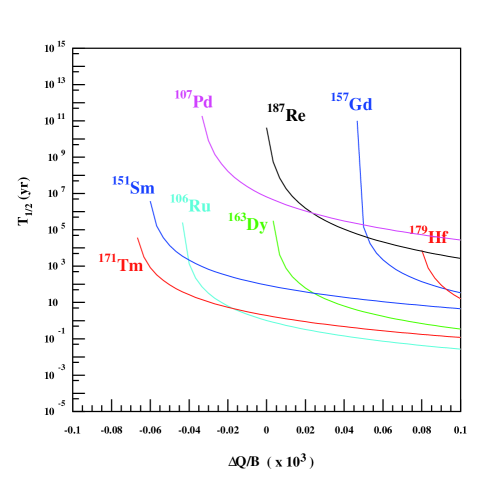
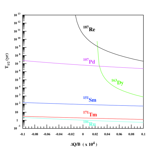
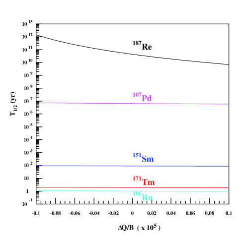
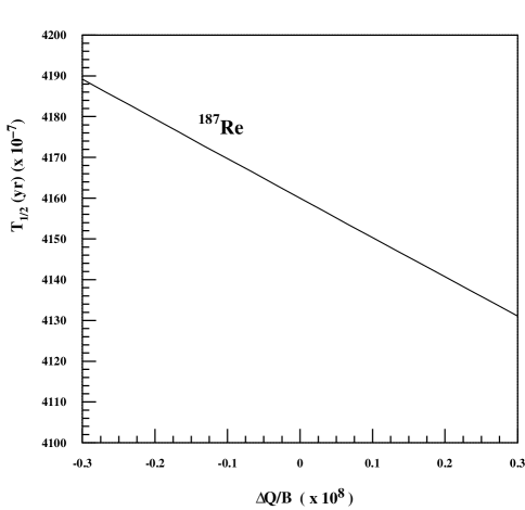
Figure 2: Evolution of half-life of the $\beta^{-}$-isotopes as a function of the $\Delta Q/B$ parameter. In a) the scale is taken to be $\Delta Q/B<10^{-3}$, in b) $\Delta Q/B<10^{-4}$, in c) $\Delta Q/B<10^{-5}$, in d) $\Delta Q/B<10^{-8}$.

3.2 Limits due to Long lived $\alpha$-decays

Dyson [27] defined the sensitivity of the decay constant of the nucleus to the change of the electromagnetic coupling constant as

$$s={\alpha\over\lambda}{d\lambda\over d\alpha},$$ (3.41)

which is a function of the decay energy $Q$. The $\alpha$-decay rate depends on $\alpha$ through the probability of Coulomb barrier penetration. Approximating this rate by

$$\lambda\propto\exp\left[-{4\pi\alpha Z\over\sqrt{Q_{\alpha}/(2m_{p})}}\right],$$ (3.42)

where $Z$ is the atomic number of the daughter nucleus, we can write

$$s=-{4\pi\alpha Z\over\sqrt{Q_{\alpha}/(2m_{p})}}\left(1-{1\over 2}u\right),$$ (3.43)

where

$$u={\alpha\over Q_{\alpha}}{dQ_{\alpha}\over d\alpha}.$$ (3.44)

The decay energy $Q_{\alpha}$ is given by

$$Q_{\alpha}=B(A,Z)+B_{\alpha}-B(A+4,Z+2),$$ (3.45)

where $B_{\alpha}$ is the nuclear binding energy of the $\alpha$-particle. Varying only the Coulomb terms in Eq. (2.9) and neglecting the contributions from $B_{\alpha}$, we obtain $s=774$, 890, 575, 659, 571, 466, and 549 for ¹⁴⁷Sm, ¹⁵²Gd, ¹⁵⁴Dy, ¹⁹⁰Pt, ²³²Th, ²³⁵U, and ²³⁸U, respectively.

The variation $\Delta\alpha/\alpha$ is related to $\Delta\lambda/\lambda$ as

$${\Delta\alpha\over\alpha}={1\over s}{\Delta\lambda\over\lambda}.$$ (3.46)

Since the values of $s$ for the nuclei listed above are similar, the most stringent constraint on $\Delta\alpha/\alpha$ is given by the nucleus with the smallest known $\Delta\lambda/\lambda$. While it is tempting to use ²³⁸U for this purpose, the uncertainty of $6.7\times 10^{-4}$ given in Table 4, corresponds to a laboratory measurement and is not directly applicable to a constraint at high redshift. Indeed, ²³⁸U is extremely well measured, and is used to calibrate the ages of the meteorites. Instead, we consider ¹⁴⁷Sm as an example, and assume that $\Delta\lambda/\lambda$ is less than the fractional meteoritic uncertainty of $7.5\times 10^{-3}$ in the half-life of ¹⁴⁷Sm [31] given in Table 4 (see also [32]). This gives

$${\Delta\alpha\over\alpha}\mathrel{\raise 1.29167pt\hbox{$<$\kern-7.5pt\lower 4.30554pt\hbox{$\sim$}}}10^{-5}.$$ (3.47)

Table 4: Sensitive and insensitive $\alpha$- and $\beta^{-}$-isotopes

Nucleus	Decay	$Q$ (MeV)	Half-life (yr)	$\Delta\lambda/\lambda_{\rm lab}$ (%)	$\Delta\lambda/\lambda_{\rm met}$ (%)
238U	$\alpha$	4.27	$4.468\times 10^{9}$	$0.067$	–
235U	$\alpha$	4.678	$7.038\times 10^{8}$	$0.071$	–
232Th	$\alpha$	4.082	$1.405\times 10^{10}$	$0.4$	$>1$
147Sm	$\alpha$	2.31	$1.06\times 10^{11}$	$1.9$	0.75
87Rb	$\beta^{-}$	0.283	$4.75\times 10^{10}$	$0.8$	$0.8$
40K	$\beta^{-}$	1.311	$1.265\times 10^{9}$	$0.6$	$1$

The change in $\lambda$ due to more general variations of the fundamental constants can be written as

$${\Delta\lambda\over\lambda}=-{4\pi\alpha Z\over\sqrt{Q_{\alpha}/(2m_{p})}}\left[{\Delta\alpha\over\alpha}+{1\over 2}\left({\Delta m_{p}\over m_{p}}-{\Delta Q_{\alpha}\over Q_{\alpha}}\right)\right].$$ (3.48)

We again take ¹⁴⁷Sm as an example, for which

$$Q_{\alpha} = 3.36T_{0}+3.40V_{V}-0.070V_{\rm sym}+39.9a_{C}-0.975C_{d}$$ (3.49)

$$+\Delta_{\rm sh}(143,60)-\Delta_{\rm sh}(147,62)+B_{\alpha},$$

where the numerical values for all the terms except for the last three on the right-hand side are 77.31, $-131.51$, $-1.08$, 28.63, $-1.18$ MeV, respectively. The experimental value of $B_{\alpha}$ is 28.30 MeV. Comparing the $Q_{\alpha}$ calculated above with the experimental value of 2.31 MeV gives an estimate of $\Delta_{\rm sh}(143,60)-\Delta_{\rm sh}(147,62)=-1.84$ MeV. We again see that changes in $T_{0}$ and $V_{V}$ produce the largest effects on $Q_{\alpha}$. Note however, that because the decay-rate depends on the ratio of $Q$ to $m_{p}$, if we neglect quark mass contributions to $Q$ and $m_{p}$ and retain only the scaling due to $\Lambda$, we see that the contributions from $\Delta m_{p}/m_{p}$ and $\Delta Q/Q$ in Eq. (3.48) cancel and no improvement in the limit is possible. Including the quark contribution through the coefficient, $\kappa$, we expect that the scaling of $T_{0}$ and $V_{V}$ with $m_{q}/\Lambda$ will not be exactly the same as that of $m_{p}$. So Eq. (3.48) gives

$${\Delta\lambda\over\lambda}\simeq-{2\pi\alpha Z\kappa\over\sqrt{Q_{\alpha}/(2m_{p})}}{T(V)\over Q_{\alpha}}{\Delta(m_{q}/\Lambda)\over(m_{q}/\Lambda)}=(3-20)\times 10^{2}\left|\frac{\Delta v}{v}-\frac{\Delta\Lambda}{\Lambda}\right|,$$ (3.50)

using ${\Delta(m_{q}/\Lambda)/(m_{q}/\Lambda)}=\left|{\Delta v}/{v}-{\Delta\Lambda}/{\Lambda}\right|$. The range is due to the difference in $T$ and $V$ (80 – 130 MeV) compared to $Q\sim 2$ MeV and the range in $\kappa=0.1-0.5$ as discussed above. The variation in Eq. (3.50) corresponds to

$${\Delta\alpha\over\alpha}<(0.8-5)\times 10^{-7}$$ (3.51)

for $\Delta\lambda/\lambda<7.5\times 10^{-3}$. As shown below, this constraint is less stringent than that derived from ¹⁸⁷Re $\beta$-decay.

3.3 Limits due to Long lived $\beta$-decays

In section 3.1, we have seen that ¹⁸⁷Re is the most sensitive indicator of a possible variation of $\alpha$ as first argued by Peebles and Dicke [33] and Dyson [27]. The upper limit obtained from the analysis of the Re/Os ratio in iron meteorites obtained at that time was $\dot{\alpha}/\alpha=5\times 10^{-15}$ yr^-1 [27], and was less stringent than the Oklo limit [11]. In spite of this, Re is of interest since the estimate of the effect of the variation of the coupling constants (particularly when we go beyond variations in $\alpha$) based on the resonance energy (in the Oklo case) is more complicated than that based on the Q value (in the Re case). As we saw in section 2, the constraints based on the Sm resonant energy required some knowledge of the role of quark masses in the nucleus and a limit based on variations of $\Lambda_{QCD}$ alone could not be obtained. In the case of $\beta$-decay, a constraint can be obtained in a more direct way. Above all, the Re analysis is independent of the Oklo analysis and uses different physics. Finally, the dramatic improvement in the meteoritic analyses of the ¹⁸⁷Re/¹⁸⁷Os ratio mandates an update of the constraint on variations of the coupling constants.

Rhenium occurs in relatively high concentration in iron rich meteorites. The ¹⁸⁷Re decay rate has been determined through the generation of high precision isochrons from material of known ages, particularly iron meteorites. Using the Re-Os ratios of IIIAB iron meteorites that are thought to have been formed in the early crystallization of asteroidal cores, Smoliar et al. [34] (see also [35]) found a ¹⁸⁷Re half-life of 41.6 Gyr within 0.5% assuming that the age of the IIIA iron meteorites is 4.5578 Gyr $\pm 0.4$ Myr which is identical to the Pb-Pb age of angrite meteorites [36]. For a general discussion see refs. [37, 32]. The results of Smoliar et al. [34] are in good agreement with those of Shen et al. [38], which adds confidence to the meteoritic value of the half-life (which is more precise than the direct measurement [39] which carries a 3% uncertainty). The ages of iron meteorites determined by Rhenium dating are in excellent agreement with other chronometers such as U-Pb and Mn-Cr, which means that the Rhenium lifetime has not varied more than 0.5% over the age of iron meteorites (4.56 Gyr). This gives $\dot{\lambda}/\lambda<1.1\times 10^{-12}$ yr^-1, to be compared with the limit of $10^{-10}$ yr^-1 given by Dyson [27]. The improvement in the data is considerable.

The $\beta$-decay of ¹⁸⁷Re is a unique first fordidden transition, for which the energy dependence of the decay rate can be approximated as [40]

$$\lambda\propto G_{F}^{2}Q_{\beta}^{3}m_{e}^{2}.$$ (3.52)

which is in agreement with [27] and gives a good description of the variation of $T_{1/2}$ with $Q_{\beta}$ shown in Fig. 2d. The decay energy, $Q_{\beta}$, is given by

$$Q_{\beta} = B(187,76)-B(187,75)+(m_{n}-m_{p}-m_{e})$$ (3.53)

$$= 0.339T_{0}+0.611V_{\rm sym}-26.4a_{C}+0.807C_{d}+\Delta_{\rm sh}(187,76)-\Delta_{\rm sh}(187,75)$$

$$+(m_{n}-m_{p}-m_{e}),$$

where $m_{n}$ is the neutron mass and the numerical values for all terms except for the last three on the right-hand side are 7.80, 9.34, $-18.93$, and 0.98 MeV, respectively. The experimental value of $(m_{n}-m_{p}-m_{e})$ is 0.78 MeV. Comparing the $Q_{\beta}$ calculated above with the experimental value of 2.66 keV gives an estimate of $\Delta_{\rm sh}(187,76)-\Delta_{\rm sh}(187,75)=0.03$ MeV. Considering only the variation of the Coulomb term in $Q_{\beta}$, we have

$${\Delta\lambda\over\lambda}=3{\Delta Q_{\beta}\over Q_{\beta}}\simeq 3\left({20\ {\rm MeV}\over Q_{\beta}}\right)\left({\Delta\alpha\over\alpha}\right)\simeq 2\times 10^{4}\left({\Delta\alpha\over\alpha}\right),$$ (3.54)

which gives $\delta\alpha/\alpha<3\times 10^{-7}$ for $\delta\lambda/\lambda<0.5\%$ over a period of 4.6 Gyr or $\dot{\alpha}/\alpha<6\times 10^{-17}$ yr^-1. This is 100 times more stringent than the constraint in [27] due to the improvement of the limit on $\dot{\lambda}/\lambda$.

The contributions to $Q_{\beta}$ from $T$ and $V$, which scale with $\Lambda$, are comparable to that from the dominant Coulomb term, which scales as $\alpha\Lambda$. As changes in $\Lambda$ are $O(30)$ times larger than that in $\alpha$, we can estimate

$${\Delta\lambda\over\lambda}=3{\Delta Q_{\beta}\over Q_{\beta}}-2{\Delta v\over v}\simeq 3{T(V,C)\over Q_{\beta}}{\Delta\Lambda\over\Lambda}\simeq 2\times 10^{4}{\Delta\Lambda\over\Lambda},$$ (3.55)

which gives

$${\Delta\alpha\over\alpha}<8\times 10^{-9}$$ (3.56)

for $\Delta\lambda/\lambda<0.5\%$ over a period of 4.6 Gyr or $\dot{\alpha}/\alpha<2\times 10^{-18}$ yr^-1.

Note that all of these limits based on Re decay hold only if the variation of $\lambda$ is of the same order as the accuracy of $\lambda$. This hypothesis can be cross-checked by different chronometric pairs with different sensitivities to variations of $\alpha$. Furthermore, we can check a posteori, that even though the meteoritic ages are determined in part by lab measurements of the ²³⁸U lifetime, the limits above still hold. To see this, we note that the adopted uncertainty in the Re half-life is determined by the uncertainty in the slope of ¹⁸⁷Os/¹⁸⁸Os vs. ¹⁸⁷Re/¹⁸⁸Os. The uncertainty in the age of the meteorites is neglected. However, Re is far more sensitive to changes in $\alpha$ than is U (ie., the sensitivity factor for U is about 500, while for Re it is 2 $\times 10^{4}$). It is relatively simple to check that a consistent limit requires changes in $\alpha$ which are sufficiently small so that the uncertainty in the meteoritic age can be neglected.

4 $s$-process nucleosynthesis

A variation of the fundamental constants could have several other significant consequences on astrophysical processes particularly on nucleosynthesis. For example, variations in the gauge couplings would affect the position of the triple $\alpha$-resonance necessary for the synthesis of ¹²C. This has been examined recently by Oberhummer et al. [41]. Here, we focus on the nucleosynthesis of heavier isotopes and in particular those generated by the $s$-process. We will keep our discussion qualitative since the nucleosynthesis of neutron rich isotopes is complex at both nuclear and stellar levels. Branching on the $s$-process path occurs every time the $\beta$-decay lifetime of a given isotope is commensurate with the neutron capture lifetime (see [42], for a review). Among the nuclei listed in table 1, several species are involved in $s$-process branching (specially in the $Sm-Eu-Gd$, $W-Re-Os$ and $Hg-Tl-Pb$ regions, on the basis of their low $Q/B$ ratio [43, 44, 45, 46]). $s$-process nucleosynthesis has been studied in the context of the classical constant temperature scenario and more realistically in connection to thermal pulses in AGB stars. In the constant temperature scenario of the classical $s$-process, thermal excitation of low lying energy states takes place, strongly modifying stellar lifetimes, and the subtle effects of the variation of the coupling constants are masked. However, more realistic models of the stellar $s$-process invoke highly convective situations during thermal pulses followed by long episodes of quietness. The AGB recurrent thermal pulses give rise to rapid mixing of freshly synthesized material in cooler zones. In these periods, the effect of variations in $\alpha$ could show up, since in the interpulse regime the thermal population of excited levels is suppressed. Thus, the situation is involved and deserves a dedicated analyses on the basis of refined nuclear networks coupled to realistic stellar models.

There is however an interesting case which benefits from the high temperatures involved, that of metastable ¹⁸⁰Ta, which is the rarest isotope in nature and is assumed to be predominantly of $s$-process origin [47, 48], (see however [49]). It is also the only isotope which is stable in the isomeric state. Would it remain metastable if the coupling constants were different in the past? This question also deserves investigation. Here, we will assume that it does remain metastable. The difficulty in producing this isotope in contrast to the facility of its destruction by thermally induced depopulation of the short lived ¹⁸⁰Ta ground state in stars is reflected in its rarity. The population of an excited state of ¹⁷⁹Hf at relatively high excitation energy ($7/2-$ at 214 keV) is crucial to the synthesis of the metastable ¹⁸⁰Ta. The decay rate of excited ¹⁷⁹Hf, in turn, is essentially dominated at high temperature by the bound state $\beta$-decay, thus a small alteration of its Q value (say by a few keV) would have strong consequences on the final Ta yield (at least in the classical $s$-process context). As the $Q_{\beta}$ value for decay from the 214 keV excited state of ¹⁷⁹Hf is $\approx 100$ keV, the variation of $\Delta Q_{\beta}/Q_{\beta}$ would be limited to less than a few percent. Comparing this with $\Delta Q_{\beta}/Q_{\beta}=(1/3)\Delta\lambda/\lambda<2\times 10^{-3}$ for ¹⁸⁷Re, we expect that the constraints derived from considerations of ¹⁷⁹Hf decay would be $\sim$ 10 times weaker than those presented in section 3.3 for ¹⁸⁷Re.

More generally, bound state $\beta$-decay is expected to occur in highly ionized media in which the decay electron has a high probability to be captured in an empty atomic orbit. It is the time reversed process of orbital (bound) electron capture. It occurs whenever Q ($<0$) is of the order of the binding energy of electrons in the innermost shells. ¹⁸⁷Os with $Q=-2.6keV$ is particularly sensitive to variations of the fundamental couplings. Other interesting cases are ¹²¹Te, ¹⁶³Dy, and ²⁰⁵Tl. Thus, in stellar conditions, new disintegration channels could open up and stable nuclei in the laboratory could become unstable. Consequently, a slight perturbation of Q values could have significant consequences on the results of the $s$-process and more importantly on the Re/Os datation [50]. Indeed, the ¹⁸⁷Re decay rate could be considerably enhanced in stellar interiors [47] by the bound beta-decay of highly ionized ¹⁸⁷Re. At typical $s$-process temperatures ($3.10^{8}$ K), the bound state $\beta$-decay of ¹⁸⁷Re in to the 9.75 keV ¹⁸⁷Os level is energetically possible, provided the degree of ionization is high. The non unique forbidden transition may give an overwhelming contribution to the ¹⁸⁷Re decay rate, non unique transitions being, in general much faster than unique ones. This effect could be easily suppressed by a slight change of $Q$ related to a change of couplings.

5 Summary

We have considered the class of unified theories in which gauge and Yukawa couplings are determined dynamically by the vacuum expectation value of a dilaton or modulus field. While such theories may allow the possibility that the fundamental coupling constants are variable (in time), they general do so in an interdependent way. That is, one expects on quite general grounds that a variation in the fine structure constant is accompanied by a variation in all gauge and Yukawa couplings. Even more importantly, as described in [15], such variations are also accompanied by variations in quantities such as $\Lambda_{QCD}$ and the Higgs expectation value which are determined from the gauge and Yukawa couplings by transdimensional mutation. Limits on the variations in these dimensionful quantities impose severe bounds on variations in the fine-structure constant. In the context of dynamical models where the change in fundamenntal parameters is goverened by a nearly massless modulus, these limits are complementary to the constraints imposed by checks of the equivalence principle.

Within this context, we have re-examined the constraints which can be obtained from the natural nuclear reactor at Oklo. The previous bound [11] of $\Delta\alpha/\alpha<10^{-7}$ was found by limiting the variations in the Coulombic contribution of the $Q$ value for the resonant neutron capture process. We found that by including variations in $Q$ which are induced by variations in $\Lambda$ and the quark masses, $m_{q}$, we can improve this bound by approximately two to three orders of magnitude. The improvement is due to 1) the sensitity of both $\Delta\Lambda/\Lambda$ and $\Delta v/v$ to $\Delta\alpha/\alpha$ (a factor of 50), and 2) the sensitivity to the dominant terms kinetic and potential terms in $Q$ rather than the Coulomb term (a factor of 30). However, we lose a factor of 2 – 5, due to the rather uncertain contributions of the quark masses to the nuclear potential in a heavy nucleus. Thus we obtain the limit $\Delta\alpha/\alpha<(1-5)\times 10^{-10}$. It is clear that this bound, which is valid at the time period corresponding to a redshift $z\simeq 0.15$, would require severe fine-tuning in any model which attempts to fit the recent quasar absorption data with $\Delta\alpha/\alpha\sim 10^{-5}$ over redshifts $z=0.5-3.5$. In particular, our results strengthen the need for the fine-tuning in Bekenstein-type models, as emphasized in [6].

We have also considered the bounds which can be derived from long-lived or barely stable isotopes. Small variations in $\alpha$ ($\Lambda$ and $v$) can lead to changes in the $Q$ value in heavy nuclei. We showed that limits from $\alpha$-decay nuclei such as ¹⁴⁷Sm can be as strong as $\Delta\alpha/\alpha<10^{-5}$ from purely Coulombic variations, and $\Delta\alpha/\alpha<(0.8-5)\times 10^{-7}$ based on ¹⁴⁷Sm life-time uncertainties as small as $\Delta\lambda/\lambda<7.5\times 10^{-3}$.

We further showed that improvements in meteoritic abundance determinations have enabled one to derive substantially stronger bounds based on the $\beta$-decay lifetimes of ¹⁸⁷Re. From the analysis of the Re/Os ratio in meteorites with ages of 4.56 Gyr (known to an accuracy of 0.01%), the half-life of ¹⁸⁷Re has been determined to an accuarcy of about 0.5%. Purely Coulombic variations in $\alpha$ lead to the bound $\Delta\alpha/\alpha<3\times 10^{-7}$. From the age of the meteorites, this limit is applicable at redshift $z=0.45$. Thus not only is it competitive with the Oklo bound numerically, but it corresponds to a higher redshift further emphasizing the difficulty in achieving a value of $\Delta\alpha/\alpha\sim 10^{-5}$ at higher redshift. We further stress that the physics involved in deriving this bound is independent to that used for the Oklo bound. When variations in $\Lambda$ are included, the bound is improved to $\Delta\alpha/\alpha<8\times 10^{-9}$.

Acknowledgments
We warmly thank J. L. Birck, G. Manhes and M. Arnould for providing us with information about meteoritic analyses, and P. Vogel, M. Galeazzi, and W. Bühring for communications on the energy dependence of ¹⁸⁷Re decay. We also thank M. Srednicki for useful conversations. This work was supported in part by DOE grants DE-FG02-94ER-40823, DE-FG02-87ER40328, and DE-FG02-00ER41149 at the University of Minnesota and by PICS 1076 CNRS France/USA. The work of M.P. is supported by P.P.A.R.C.

References

- [1]
- [2] J.K. Webb et al., Phys. Rev. Lett. 87 (2001) 091301.
- [3] A. V. Ivanchik, E. Rodriguez, P. Petitjean and D. A. Varshalovich, arXiv:astro-ph/0112323.
- [4] J. D. Bekenstein, Phys. Rev. D 25 (1982) 1527.
- [5] H. B. Sandvik, J. D. Barrow and J. Magueijo, arXiv:astro-ph/0107512; J. D. Barrow, H. B. Sandvik and J. Magueijo, arXiv:astro-ph/0109414.
- [6] K. A. Olive and M. Pospelov, Phys. Rev. D 65, 085044 (2002) [arXiv:hep-ph/0110377].
-
[7]
R.V. Eötvös, V. Pekar and E. Fekete, Ann. Phys. (Leipzig)
68 (1922) 11;
P. G. Roll, R. Krotkov and R. H. Dicke, Annals Phys. 26 (1964) 442;
V.B. Braginsky and V.I. Panov, Zh. Eksp. Teor. Fiz. 61 (1972) 873 [Sov. Phys. JETP 34 (1972) 463. - [8] M. Livio and M. Stiavelli, Ap. J. Lett. 507 (1998) L13.
- [9] P. Sisterna and H. Vucetich, Phys. Rev. D 41 (1990) 1034.
- [10] A. I. Shlyakhter, Nature 264 (1976) 340.
- [11] T. Damour and F. Dyson, Nucl. Phys. B 480 (1996) 37.
- [12] Y. Fujii et al., Nucl. Phys. B573 (2000) 377.
- [13] S. J. Landau and H. Vucetich, astro-ph/0005316; N. Chamoun, S. J. Landau and H. Vucetich, Phys. Lett. B 504 (2001) 1.
- [14] E. W. Kolb, M. J. Perry and T. P. Walker, Phys. Rev. D 33, 869 (1986); R. J. Scherrer and D. N. Spergel, Phys. Rev. D 47, 4774 (1993); L. Bergstrom, S. Iguri and H. Rubinstein, Phys. Rev. D 60, 045005 (1999) [arXiv:astro-ph/9902157]; K.M. Nollett and R.E. Lopez, astro-ph/0204325.
- [15] B. A. Campbell and K. A. Olive, Phys. Lett. B 345, 429 (1995) [arXiv:hep-ph/9411272].
- [16] T. Banks, M. Dine and M. R. Douglas, Phys. Rev. Lett. 88 (2002) 131301. See also Z. Chacko, C. Grojean and M. Perelstein, arXiv:hep-ph/0204142.
- [17] T. Damour and A. M. Polyakov, Nucl. Phys. B 423, 532 (1994).
- [18] V.V. Dixit and M. Sher, Phys. Rev. D37 (1988) 1097.
- [19] P. Langacker, G. Segre and M. J. Strassler, Phys. Lett. B 528, 121 (2002) [arXiv:hep-ph/0112233].
- [20] K. Ichikawa and M. Kawasaki, arXiv:hep-ph/0203006.
- [21] T. Dent and M. Fairbairn, arXiv:hep-ph/0112279; X. Calmet and H. Fritzsch, arXiv:hep-ph/0112110; arXiv:hep-ph/0204258; T. Damour, F. Piazza and G. Veneziano, arXiv:gr-qc/0204094; arXiv:hep-th/0205111.
- [22] M. A. Preston and R. K. Bhaduri, “Structure of the Nucleus,” Addison-Wesley (1975).
- [23] V. V. Flambaum and E. V. Shuryak, Phys. Rev. D 65 (2002) 103503.
- [24] J. Gasser, H. Leutwyler, and M. E. Sainio, Phys. Lett. B253 (1991) 252; M. Knecht, hep-ph/9912443.
- [25] U. van Kolck, Prog. Part. Nucl. Phys. 43 (1999) 337.
- [26] K. Takahashi and K. Yokoi, Nucl. Phys. A404, 578 (1983).
- [27] F.J. Dyson, in Aspects of Quantum Theory edited by A. Salam and E.P. Wigner (Cambridge U. Press), p. 213 (1972).
- [28] G. Audi, O. Bersillon, J. Blachot and A.H. Wapstra, Nucl. Phys. A 624, 1 (1997).
- [29] A. deShalit and H. Feshbach, in “Theoretical Nuclear Physics”, John Wiley & Sons, (1974).
- [30] F.B. Shull and E. Feenberg, Phys. Rev. 75, 1768 (1949).
- [31] J. K. Tuli, “Nuclear Wallet Cards,” (6th Edition, 2000).
- [32] F. Begemann et al., Geochimica. Cosmochimica. Acta, 65, 111 (2001).
- [33] P.J. Peebles and R.H. Dicke, Phys. Rev., 128, 2006 (1962).
- [34] M.I. Smoliar et al., Science, 271, 1099 (1996).
- [35] T. Faestermann, 1998, Nuclear Astrophics 9, MPA-report P10, eds W. Hillebrandt and E. Muller, p172.
- [36] G.W. Lugmair and and J.G. Galer, Geochimica. Cosmochimica. Acta, 56, 1673 (1992).
- [37] J.L. Birck, in ”Astrophysical ages and dating methods”, Edts E. Vangioni-Flam et al., Edts Frontiere, p. 427 (1989).
- [38] J.J. Shen, D.A. Papanastassiou and J. Wasserburg, Geochimica et Cosmochimica Acta, 60, 2887 (1996).
- [39] M. Lindner et al., Geochimica. Cosmochimica. Acta, 53, 1597 (1989).
- [40] M. Galeazzi, F. Fontanelli, F. Gatti, and S. Vitale, Phys. Rev. C, 63, 014302 (2000).
- [41] H. A. Oberhummer et al., Science, 289, 88 (2000).
- [42] F. Kappeler, H. Beers and K. Wisshak, Rep. Prog. Phys. 52, 495 (1989).
- [43] H. Beer and R.L. Macklin, Ap.J. 331, 1047 (1988).
- [44] F. Kappeler et al., Ap.J. 366, 605 (1991).
- [45] M. Arnould, K. Takahashi and K. Yokoi, A.A., 137, 51 (1984).
- [46] K. Yokoi, K. Takahashi and M. Arnould, A.A., 145, 339 (1985).
- [47] K. Yokoi and K. Takahashi, Nature, 305, 198 (1983)
- [48] K. Wisshak et al., Phys. Rev. Lett., 87, 251102 (2001)
- [49] M. Rayet et al., A.A. 298, 517 (1995)
- [50] M. Arnould and S. Goriely, in ”Astrophysical Ages and Time Scales” ASP Conference Series, in press (2002)