Time advancement in resonance regions of $\pi N$ scattering

Abstract

We evaluate the time delay in some of the established resonance regions of $\pi N$ elastic scattering. In addition to the positive peaks corresponding to resonances, we identify broad regions of negative time delay or time advancement which restrict the energy ranges within which the resonances can be located.

PACS numbers: 14.20.Gk, 11.80.Et, 13.30.Eg
Keywords: resonance parameters, time delay, partial wave analysis

I Introduction

The precise definition of a resonance has been a matter of much debate in literature (see [1] and references therein). The notion of a resonance not being so clear, different criteria are used for identifying resonances and determining their parameters. Conventionally, the baryon resonances are identified by analyzing the meson baryon scattering data using partial wave techniques. The resonance parameters (eg. those listed in the Summary Table (ST) of the Particle Data Group [2]) are determined by fitting some energy dependent functional form such as the Breit-Wigner to the scattering amplitude. The resonances are then located using techniques such as the Argand diagrams and Speed Plots [3, 4] of the energy dependent complex amplitude. In contrast to these conventional procedures we make use of one of the basic criteria for the existence of a resonance, namely, a positive peak in the time delay in collisions. Intuitively one would expect the scattering particles to be held up for a while due to the formation and decay of a resonance, leading to a positive time delay peaked in energy around the resonance mass. This time delay as we shall see below is related to the lifetime of a resonance. In fact, in ref.[5], where the authors discuss several criteria for identifying resonances, it was noted that a bump in the cross section may not always be due to a resonance, but a sharp maximum in time delay is sufficient condition for the existence of a resonance.

An exploratory study of the time delay in $\pi N$ elastic scattering led us to an interesting finding, namely, the observation of negative time delay or time advancement in some resonance regions of $\pi N$ elastic scattering. Though we find positive peaks within the mass range specified for the resonance (by the ST), these peaks are surrounded by regions of negative time delay, thus restricting the possible mass range for the resonance. Contrary to our understanding of relating a resonance with time delay, we observe that the resonances identified by some of the conventional analyses fall in the regions of time advancement. We wish to emphasize that it has been mentioned in literature as well as text books [6] that a positive time delay is necessary for the existence of a resonance. The present work identifies those energy regions which do not satisfy this criterion and also those analyses which do not fulfill this necessary condition.

II Time delay and S-matrix

The formation of a resonance which occurs as an unstable intermediate state in scattering processes, introduces a time delay between the arrival of the incident wave packet and its departure from the collision region. Using a wave packet analysis in the early fifties, it was shown by Bohm [7], Eisenbud [8] and Wigner [9], that the time delay $\Delta t$ in collisions can be defined in terms of the energy derivative of the scattering phase shift as follows:

$$\Delta t(E)=2\hbar{d\delta(E)\over dE}\,.$$ (1)

The connection between the lifetime matrix and S-matrix was later established by Smith [10] and it was shown that the time delay for a particle injected in the $i^{th}$ channel and emerging in the $j^{th}$ channel is given in terms of the S-matrix as,

$$\Delta t_{ij}(E)=Re\big{[}-i\hbar(S_{ij})^{-1}{dS_{ij}\over dE}\big{]}\,.$$ (2)

Using a phase shift formulation of the S-matrix, we get,

$$\Delta t_{ii}(E)=2\hbar{d\delta(E)\over dE}$$ (3)

by substituting $S_{ii}=e^{2i\delta}$ in eq. (2). This is exactly the relation mentioned in eq. (1). The scattering phase shift $\delta$ is real. The time delay $\Delta t_{ii}(E)$ is actually the lifetime of metastable states or resonances in elastic scattering.

At high energies, in addition to elastic scattering, several inelastic channels open up, giving rise to multichannel resonances. The S-matrix is then modified and defined as $S=\eta e^{2i\delta}$, where $\eta$ is the inelasticity parameter such that, $0\leq\eta\leq 1$. By substituting the modified $S$ in the expression for $\Delta t_{ii}$ in eq. (2), we obtain the time delay in elastic scattering, in the presence of inelastic channels. It can be easily checked that even with the modified $S$, $\Delta t_{ii}=2\hbar{d\delta(E)\over dE}$ as in the purely elastic case. The phase shift $\delta$ is still real, but its value is affected by the presence of the inelastic channels.

The average time delay for a particle injected in the $i^{th}$ channel (assuming that it has a probability $|S_{ij}|^{2}$ of emerging into the $j^{th}$ channel) is given as [10],

$$<\,\Delta t_{i}\,>_{av}=\sum_{j}\,S_{ij}^{*}S_{ij}\Delta t_{ij}$$ (4)

Separating the contributions of the elastic and inelastic channels, we get,

$$<\,\Delta t_{i}\,>_{av}=\eta^{2}\Delta t_{ii}\,+\,\sum_{j\neq i}\,S_{ij}^{*}S_{ij}\,\Delta t_{ij}\,.$$ (5)

Thus we see that, in the absence of inelastic channels (i.e. when the resonance formed from the $i^{th}$ channel decays with a 100% branching fraction into the $i^{th}$ channel) $\Delta t_{ii}$ gives the full lifetime of the resonance, while in general, in the presence of inelastic channels, the time delay $\Delta t_{ii}$ is associated with the partial lifetime of a multichannel resonance which decays back to the channel from which it originated.

Instead of using the phase shift formulation of the S-matrix, one could also start by defining the S-matrix in terms of the T-matrix as,

$$S=1+2iT\,$$ (6)

as is usually done in the partial wave analyses of resonances [11, 12]. The matrix $T$ contains the entire information of the resonant and non-resonant scattering and is complex ($T=T^{R}+iT^{I}$). Now, substituting for $\Delta t_{ij}$ from eq. (2) into eq. (4) for the average time delay, we get,

$$<\,\Delta t_{i}\,>_{av}=Re\big{[}-i\hbar\sum_{j}(S_{ij})^{*}{dS_{ij}\over dE}\big{]}$$ (7)

which, with the substitution of the S-matrix of eq. (6) gives,

$$<\,\Delta t_{i}\,>_{av}=\sum_{j}2\hbar\biggl{[}{dT^{R}_{ij}\over dE}+2T^{R}_{ij}{dT^{I}_{ij}\over dE}-2T^{I}_{ij}{dT^{R}_{ij}\over dE}\biggr{]}.$$ (8)

From the above equation we see that in addition to the possibility of evaluating time delay from the scattering phase shifts, we can also evaluate it using an energy dependent amplitude $T$. The time delay $\Delta t_{ii}$, in terms of the real and imaginary parts of the amplitude $T$ is given as,

$$S^{*}_{ii}S_{ii}\,\Delta t_{ii}=2\hbar\biggl{[}{dT^{R}_{ii}\over dE}+2T^{R}_{ii}{dT^{I}_{ii}\over dE}-2T^{I}_{ii}{dT^{R}_{ii}\over dE}\biggr{]},$$ (9)

where $S^{*}_{ii}S_{ii}$ can be evaluated using eq. (6).

In what follows, we shall evaluate the time delay in $\pi N$ elastic scattering. We have checked that the values of time delay, $\Delta t_{ii}$, obtained either using the derivative of the real phase shifts as in eq. (3) or the T-matrix as in eq. (9) are the same. We shall initially show the time delay plots evaluated using fits to the single energy values of the scattering amplitude and identify in addition to the resonances, regions of negative time delay. Later on, choosing the energy dependent solution of a particular analysis [12], we demonstrate that the time delay evaluated using their complex amplitude is negative exactly in the regions where they locate the resonant poles.

Before we proceed to the results, we note that the energy derivative of the phase shift is related to the change in the density of states at a given energy due to interaction [13].

$$\sum_{l}g_{l}(E)-g_{l}^{o}(E)=\sum_{l}{2l+1\over\pi}\,{d\delta_{l}(E)\over dE}$$ (10)

where $g_{l}(E)$ and $g_{l}^{o}(E)$ are the densities of states with and without interaction respectively. We can see from the above equation that if $\delta_{l}$ (phase shift in the $l^{th}$ partial wave) rises steeply over a narrow energy range and then flattens, it will give rise to a rapid increase in the density of states. Since $d\delta_{l}/dE$ is related to the time delay $\Delta t(E)$, in the resonance region where $\Delta t(E)$ is large and positive, $g_{l}(E)$ is much larger than $g_{l}^{o}(E)$. The negative time delay or time advancement would correspond to situations where due to interaction, the density of states is less than in the absence of interaction. We shall come back to this point later.

III Time delay in $\pi N$ elastic scattering

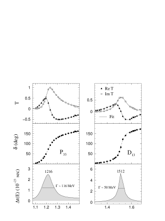
FIG. 1.: Single energy values of the partial wave amplitude (T), scattering phase shifts ($\delta$) and the time delay ($\Delta t_{ii}$ of eqs. (3) and (9)) for the $P_{33}$ and $D_{13}$ partial waves in $\pi N$ elastic scattering. The time delay is evaluated using fits (solid lines) to the single energy values of $T$.

To demonstrate the validity of the method, we first plot the lifetime of some of the well known baryon resonances. In Fig. 1 are shown the scattering amplitude ($T$) and phase shifts ($\delta$) for the $P_{33}$ and $D_{13}$ partial waves in $\pi N$ scattering (partial wave notation: $L_{2I,2J}$), in the energy region around the two known resonances, $\Delta(1232)$ and $N(1520)$. Using fits which pass through the single energy values of $T$, extracted from the cross section data [14], we evaluate the lifetime distribution $\Delta t(E)$ for the 2 cases mentioned above. Both resonances show up as distinct peaks in $\Delta t(E)$ as a function of energy. The widths of the $P_{33}$ and $D_{13}$ peaks at half maximum can be read from Fig. 1 to be around 116 and 50 MeV respectively. The peaks in their lifetime distributions occur at 1216 and 1512 MeV respectively. In the case of $\Delta(1232)$ which has 99% fraction of its decay to the $\pi N$ mode, the $\Delta t(E)$ plot gives the full width of this resonance. In the other case, the width of the peak in the $\Delta t(E)$ distribution is the partial width corresponding to 50-60% decay to the $\pi N$ mode as listed in the ST.

We have seen in Fig. 1, that in the energy regions close to resonances, the time delay is large and positive. One can say that the incident particle is held up by the scatterer for some time. It is also possible that the interaction between the beam and scatterer is such that the incident particle is accelerated through the central region of scattering. This would lead to a time advancement or negative value of time delay. Alternatively, if we consider the interpretation of time delay in terms of the density of states as in eq. (10), then a negative value of time delay would mean a reduction in the density of states, or a loss of flux from the channel under consideration. In the present work, we are interested in calculating the energy distribution of the time delay in elastic scattering. At energies corresponding to the opening up of inelastic channels, we expect that the loss of flux from the elastic channel will give rise to negative values of time delay. A negative dip in the energy distribution of time delay is thus expected at the energy corresponding to maximum inelasticity. However, in the event that an inelastic channel opens up with the formation of a resonance which can also decay to the elastic channel, we will not see a dip but rather a positive peak due to the resonance. For example, the inelasticity in the $D_{13}$ partial wave (or in other words, the reaction cross section) reaches a maximum at $E\sim 1520$ [14]; however, the presence of the resonance does show up as a peak in $\Delta t(E)$ as seen in Fig. 1. $S_{11}$ resonance region Let us first consider the $S_{11}$ resonance region in $\pi N$ elastic scattering. The well known resonance $N(1535)$ in the $S_{11}$ partial wave, apparently plays a very important role in several reactions at intermediate energies. It has very often been incorporated in theoretical models aimed at explaining $\eta$-meson production and those investigating the possibility of the formation of $\eta$-mesic nuclei. The fractional decay of this resonance is listed in the ST to be 35-55% for both the $N^{*}\rightarrow\pi N$ and $N^{*}\rightarrow\eta N$ decay modes. In Fig. 2a (left half of Fig. 2) we plot the $\pi N$ amplitude ($T$), scattering phase shifts ($\delta$) and the energy distribution of the lifetime calculated from the fit (solid line) made to the single energy values of $T$. We observe a negative dip in time delay around E = 1535 MeV.

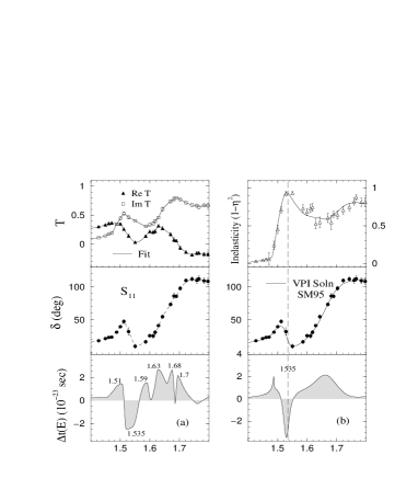
FIG. 2.: (a) Same as Fig. 1, but for $S_{11}$ partial wave. (b) Single energy values of inelasticity (1 - $\eta^{2}$) (open triangles), the phase shifts (filled circles) and the energy dependent solutions of the VPI group (solid lines). The time delay in the lower part is evaluated using the VPI solutions.

In the right half, i.e. in Fig. 2b, we show the energy dependent solutions of the VPI group [12] (solid lines passing through the single energy values of phase shifts and inelasticities) and the time delay evaluated using their solution for $T$. The time delay appears to be similar as in Fig. 2a except for the resonance region around 1650 MeV. The smooth VPI solutions give rise to a single resonance around 1650 MeV, whereas, the fit in Fig. 2a gives rise to 4 resonances in this region. The 4 peaks are located at 1.59, 1.63, 1.68 and 1.7 GeV. It could be a matter of debate whether making a fit to the detailed structure of the single energy values of phase shifts or $T$ (which gives rise to the 4 peaks) is reasonable. However, there is some support to this structure from recent works in literature [15, 16], where the existence of new resonances at 1.6 and 1.7 GeV is predicted within quark models.

Coming back to the negative dip around 1535, it can be seen from Fig. 2b that this dip occurs at an energy corresponding to the peak in inelasticity. We see from eq. (3) and also from Fig. 2 that the falling phase shift gives rise to negative time delay, thus ruling out the existence of a resonance in that energy region. This observation is different from that of ref. [3] which is based on Speed Plots, which as we shall see later are not time delay plots.

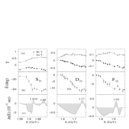
FIG. 3.: Same as Fig. 1 but for the $S_{31}$, $D_{33}$ and $F_{35}$ partial waves in $\pi N$ elastic scattering.

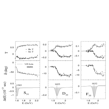
FIG. 4.: Same as Fig. 3 with the difference that the time delay is evaluated using the VPI solutions (solid lines passing through the single energy values of $T$). The numbers above the arrowheads indicate the pole positions of $T$ quoted by this group [12]. All three values lie in regions of negative time delay.

Established regions of $\Delta$ resonances In Fig. 3 we plot the energy distribution of time delay in the $S_{31}$, $D_{33}$ and $F_{35}$ partial waves of $\pi N$ elastic scattering. The time delay shown in the figure is evaluated using the dashed curves which are fits made to the single energy values of phase shifts. We repeat again that the time delay evaluated using the amplitude $T$ instead of phase shifts (eq. (9)) is the same. The known resonances occuring in these partial waves in the energy regions shown in the figure are the $\Delta(1620)$, $\Delta(1700)$ and $\Delta(1905)$ respectively, as listed by the Particle Data Group. They have been assigned 4 stars in the ST and are hence supposed to be well established. However, even when the resonances are well established, there is a large difference in the values of the mass or pole positions as reported by different analyses. We find two peaks in the $S_{31}$ partial wave at 1624 and 1680 MeV, one peak in $D_{33}$ at 1770 MeV and one in the $F_{35}$ at 1920 MeV. The widths of these peaks are listed in Table I. Some of these peaks and widths in the time delay plots match with the resonance masses and partial widths quoted by Cutkosky and Manley (see Table II). There are however broad regions of negative time delay in all the three partial waves. The resonances identified by some of the analyses fall in the regions of negative time delay shown in Fig. 3. We list such cases (bold faced numbers) in Table II.

At this point it is necessary to add a word of caution regarding the time delay evaluated from the fits made to the single energy values of $T$. Since these fits are not analytic in nature, the occurence and positions of the resonant peaks arising from small changes in the single energy values (like the 4 peaks in Fig. 2a and the $F_{35}$ resonance in Fig. 3) can change depending on the cross section data considered to extract the single energy values. It could be useful to focus on such regions and obtain more precise cross section data to define precisely the unallowed regions of negative time delay and hence more precise values of the resonance masses.

In Fig. 4 we plot the phase shift solutions and amplitude $T$ of Arndt et al. [12] (VPI group) and the time delay evaluated using these solutions. The resonance masses identified by this group are as given in Table II. However, the time delay evaluated from their solutions of $T$, around these masses is negative. Since a positive value of time delay is a necessary condition for the existence of a resonance, one would expect that the energy dependent T-matrix which is used to locate resonances should give rise to positive time delay and not time advancement in the energy regions identified as resonance regions by the same T-matrix.

IV Ambiguity of Speed Plots

The method of Speed Plots [3, 4] involves the definition of a quantity,

$$SP(E)=\Biggl{|}{dT(E)\over dE}\Biggr{|}$$ (11)

which is called the speed of the complex partial wave amplitude $T(E)$ in the Argand diagram. In ref. [4] it is mentioned that “a pronounced maximum of $SP(E)$ indicates a maximum of the time delay, i.e. the formation of an unstable excited state”. It is clear from eqs. (8) and (9) that such an interpretation of $SP(E)$ is ambiguous since $SP(E)$ and the time delay $\Delta t$ are not the same. Since the definition in eq. (11) involves a modulus, it is clear that bumps in Speed Plots are always positive. This is not the case with time delay and in fact as shown in Table II, some of the resonances identified by Speed Plots fall in regions of negative time delay.

In conclusion, we mention that it is important to consider the criterion of positive time delay in the extraction of resonances. A detailed discussion of the time delay plots in $\pi N$ scattering is done elsewhere [17]. We believe that the existence of a positive time delay should go as a constraint in the conventional analyses. If a certain analysis generates an energy dependent T-matrix and identifies resonances using this T-matrix, then it should be made sure that the same T-matrix also gives rise to a positive time delay in the resonance regions. The observation of time advancement narrows down the energy regions over which one would expect the resonances to exist, thus making resonance determination more precise. The precise determination of resonance parameters is necessary for a better understanding of several phenomena which proceed through resonance formation.

TABLE I.: Peak positions in lifetime, corresponding widths and regions of negative time delay or time advancement in some resonance regions of $\pi N$ elastic scattering.

	$L_{2I,2J}$	Peak position	Width	Regions of time
		(MeV)	(MeV)	advancement
	$S_{11}$	1510	37.8	1513 to 1562
	$S_{11}$	1590	25.2
	$S_{11}$	1630	$\sim$ 40
	$S_{11}$	1680	$\sim$ 24
	$S_{11}$	1700	25.6
	$S_{31}$	1624	4.8	1557 to 1618
	$S_{31}$	1680	12.7	1630 to 1667
	$D_{33}$	1770	17.2	1550 to 1755
	$F_{35}$	1920	16.7	1766 to 1906

TABLE II.: Resonance masses from different analyses [2] listed in the Summary Table. Numbers indicated in bold face are the masses identified in regions of negative time delay given in Table I. Masses are in MeV.

	$L_{2I,2J}$	Manley	Cutkosky	Speed Plot	Arndt (PWA)
		B-W mass	B-W mass	pole	pole
	$S_{11}$	1534$\pm$7	1550$\pm$40	1487	1510$\pm$10
	$S_{31}$	1672$\pm$7	1620$\pm$20	1608	1585
	$D_{33}$	1762$\pm$44	1710$\pm$30	1651	1655
	$F_{35}$	1881$\pm$18	1910$\pm$30	1829	1832

I am very grateful to M. Nowakowski for many useful discussions which have helped in improving this work and to R. A. Arndt, R. S. Bhalerao, J. C. Sanabria and K. P. Khemchandani for critical comments. I wish to thank S. R. Jain for inspiring discussions on time delay.

REFERENCES

- [1] R. H. Dalitz and R. G. Moorhouse, Proc. Roy. Soc. Lond. A 318 (1970) 279.
- [2] D. E. Groom et al., The European Physical Journal C 15 (2000) 1 and 1999 off-year partial update for the 2000 edition (URL: http://pdg.lbl.gov).
- [3] G. Höhler, Newsletter 14 (1998) 168.
- [4] G. Höhler, Newsletter 9 (1993) 1.
- [5] H. C. Ohanian and C. G. Ginsburg, Am. Journal of Phys. 42 (1974) 310.
- [6] B. H. Bransden and R. Gordon Moorhouse, The Pion-Nucleon System (Princeton University Press, New Jersey, 1973); M. L. Goldberger and Watson, Collision Theory (John Wiley, 1964); C. J. Joachain, Quantum Collision Theory (North-Holland, 1975).
- [7] D. Bohm, Quantum Theory (Prentice-Hall, New York, 1951).
- [8] L. Eisenbud, dissertation, Princeton, June 1948 (unpublished).
- [9] E. P. Wigner, Phys. Rev. 98 (1955) 145.
- [10] F. T. Smith, Phys. Rev. 118 (1960) 349.
- [11] D. M. Manley and E. M. Saleski, Phys. Rev. D 45 (1992) 4002.
- [12] R. A. Arndt et al., Phys. Rev. C 52 (1995) 2120.
- [13] E. Beth and G. E. Uhlenbeck, Physics 4 (1937) 915; K. Huang, Statistical Mechanics (Wiley, New York, 1963).
- [14] Phase shifts and amplitudes can be obtained on internet (http://gwdac.phys.gw.edu).
- [15] B. Saghai and Z. Li, nucl-th/0202007; B. Saghai and Z. Li, Eur. Phys. J. A 11, 217 (2001).
- [16] Z. Li and R. Workman, Phys. Rev. C 53 (1996) R549.
- [17] N. G. Kelkar, S. R. Jain and K. P. Khemchandani, (manuscript under preparation).