O.P.E. AND POWER CORRECTIONS ON THE Q.C.D. COUPLING CONSTANT

The running coupling constant can be estimated by computing gluon two- and three-point Green functions from the lattice. Computing in lattice implies working in a fixed gauge sector (Landau). An source of systematic uncertainty is then the contribution of non gauge-invariant condensates, as $\langle A^{2}\rangle$, generating power corrections that might still be important at very high energies. We study the impact of this gluon condensate on the analysis of gluon propagator and vertex lattice data and on the estimate of $\Lambda_{\overline{\rm MS}}$. We finally try a qualitative description of this gluon condensate through the instanton picture.

1 The running coupling constant from the lattice

That the running coupling constant can be extracted from the three-gluon vertex in the Landau gauge was proposed several years ago in a seminal work $\!{}^{{\bf?}}$. The key lies on the appropriate choice of renormalisation scheme: the so-called Momentum Substraction (MOM) schemes are defined such that all the renormalised Green functions take their tree-level expressions after replacing bare by renormalised constants. Then

$$g_{R}(k^{2}) = \frac{G^{(3)}(k_{1}^{2},k_{2}^{2},k_{3}^{2})}{\left(G^{(2)}(k^{2})\right)^{3}}\ \left(Z^{\rm MOM}(k^{2})\right)^{3/2}$$ (1)

where $G^{(2)}$ and $G^{(3)}$ are the scalar form factor of two- and three-gluon Green functions and $Z^{\rm MOM}$ is the gluon propagator renormalisation constant. Alternative kinematics for the renormalisation point are possible, mainly two among them: symmetric ($k_{1}^{2}=k_{2}^{2}=k_{3}^{2}=k^{2}$) and asymmetric ($k_{1}^{2}=k_{2}^{2}=k^{2}$,$k_{3}^{2}=0$). Analysis of lattice computations of these Green functions renormalised in both yielded $\!{}^{{\bf?}}$ the estimates of the coupling and $\Lambda_{\overline{\rm MS}}$ collected in Table 1. Concerned as we were by the determination and renormalisation of the gluon propagator for the analysis of the three-point Green Function, we exploited $\!{}^{{\bf?}}$ the first by matching the data to the three-loop perturbative prediction and hence estimate a purely perturbative coupling and $\Lambda_{\overline{\rm MS}}$. The disagreement between estimates from both gluon vertex and propagator (see Table 1) manifests the impact of some ucontrolled systematic uncertainty. Even worse, the so estimated $\Lambda_{\overline{\rm MS}}$ does not behave as a scale invariant!!

Table 1: Estimates of the coupling and $\Lambda_{\overline{\rm MS}}$ from two- and three-point Green function methods .

	Three-point	Two-point
$\alpha(4.3\rm{GeV})$	0.269(3)
$\Lambda_{\overline{\rm MS}}(4.3\rm{GeV})$	299(7)
$\alpha(9.6\rm{GeV})$	0.176(2)	0.193(3)
$\Lambda_{\overline{\rm MS}}(9.6\rm{GeV})$	266(7)	319(14)

If one empirically adds a $1/p^{2}$ power correction to the perturbative formulae (we work at three loops)

$$G(p^{2})=G(p^{2})_{\rm 3loops}\left(1+\frac{c}{p^{2}}\right)\ \ \ ,\ \ \ \alpha_{s}(p^{2})=\alpha_{s}(p^{2})_{\rm 3loops}\left(1+\frac{c^{\prime}}{p^{2}}\right)\ ,$$ (2)

success is gained both in obtaining estimates by two- and three-point methods that agree to each other and in restoring the scale invariance of the estimated $\Lambda_{\overline{\rm MS}}$ parameter $\!{}^{{\bf?}}$ (see fig. 1.a). A third outcome arises from matching to Eq. 2: the estimate of $\Lambda_{\overline{\rm MS}}$ results 237(4) MeV (only the statistical error is quoted), in astonishing agreement with Schröedinger functional’s $\!{}^{{\bf?}}$: 238(19) MeV !!

   
(a) (b)

   

Figure 1: In plot (a), the upper solid points are for the estimates of $\Lambda_{\overline{\rm MS}}$ obtained through the non perturbative couplings directly computed from lattice Green functions. The lower ones are obtained through $\alpha_{s}^{\rm pert}$ in Eq. 2 by the substraction of the fitted power contribution. Plot (b) shows the best fit of lattice data for the coupling renormalised in asymmetric MOM to Eqs. 2, 3.

2 The O.P.E. picture

How large should $c$ and $c^{\prime}$ are? The Operator Product Expansion (0PE) can be invoked to let us gain some physical insight into the matter of these coefficients. The sum rule approach connects the power corrections to any non-local matrix element and the QCD vacuum expectation value of the local operators from the expansion, the so-called condensates, and gives the prescription to compute perturbatively the coefficients of the expansion (Wilson coefficients). Symmetries and power counting tell us that the gluon condensate $\langle A^{2}\rangle$ gives the major contribution to our gluon Green functions. This is of course a non gauge-invariant contribution but, as far as we work in a fixed gauge, Landau gauge, non-vanishing contributions from gauge-dependant condensates, i.e. $\langle A^{2}\rangle$, should be expected $\!{}^{{\bf?}}$. Then, our coefficients $c$ and $c^{\prime}$ can be computed $\!{}^{{\bf?}}$ (see fig. 2 ) and written in terms of the gluon condensate renormalised at any momentum scale $\mu$,

$$c^{\prime}=\chi\ c\ \ ,\ \ \ c\ =\frac{6\pi^{2}}{\beta_{0}(N_{c}^{2}-1)}\left(\ln{\frac{p}{\Lambda}}\right)^{\frac{\gamma_{0}+\widehat{\gamma}_{0}}{\beta_{0}}-1}\ \langle A^{2}\rangle_{\mu}\left(\ln{\frac{\mu}{\Lambda}}\right)^{-\frac{\gamma_{0}+\widehat{\gamma}_{0}}{\beta_{0}}}\ ;$$ (3)

   

   

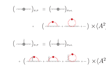
Figure 2: Diagrams in the OPE expansion of gluon two- and three-point Green functions.

with $\gamma_{0}=13/2,\beta_{0}=11,\widehat{\gamma}_{0}=3N_{C}/4$. The factor $\chi$ depends on the particular kinematics we choose for the vertex renormalisation point; case asymmetric: $\chi=1$, case symmetric: $\chi=3$.

Then, Eqs. 2, 3 are at our disposal for trying a coherent description of gluon propagator and vertex lattice data, with the sole necessity of fitting two ingredients of non-perturbative nature: $\langle A^{2}\rangle$ and $\Lambda_{\overline{\rm MS}}$ (except for an overall factor in the propagator analysis). We expand purely perturbative series up to the third loop and only keep the leading logarithm contribution for the Wilson coefficient. Of course this does not guarantee us to reach the asymptotic regime where expansions well behave. Thus, we approach the problem through a combined analysis of both gluon propagator and vertex, where we look for fitting the same $\Lambda_{\overline{\rm MS}}$ parameter in both and two independent estimates of $\langle A^{2}\rangle$ to be compared. The results of applying this to our lattice data $\!{}^{{\bf?}}$ are in Table 2. The best fit parameters lead, for instance in the case of the MOM asymmetric vertex, to the plot (b) in fig. 1.

Table 2: Comparison of results obtained to the renormalisation momentum scale $\mu=10$ GeV.

	asymmetric MOM	symmetric MOM
$\Lambda_{\overline{\rm MS}}$	260(18) MeV	233(28) MeV
$\left\{\sqrt{\langle A^{2}\rangle_{R,\mu}}\right\}_{prop}$	1.39(14) GeV	1.55(17) GeV
$\left\{\sqrt{\langle A^{2}\rangle_{R,\mu}}\right\}_{alpha}$	2.3(6) GeV	1.9(3)GeV

Consequently, the contribution of this non gauge-invariant condensate $\langle A^{2}\rangle$ seems to explain rather well the systematic deviation in the matchings of our gluon propagator and vertex lattice data to purely perturbative formulae.

3 Instantons and $\langle A^{2}\rangle$ condensate

The physical origin of this gluon condensate is a major question. A common belief is that an instanton ensemble (liquid or gas) provides with a fair description of important features of the QCD vacuum. Then, if one considers a hard gluon of momentum $p_{\mu}$ propagating in an instanton gas background (we crudely assume that instantons do not interact to each other), the propagator can be computed with Feynman graphs and it is easy to see that the dominant contribution coming from its interaction wiht the instanton gauge field is $O(1/p^{2})$ when the gauge field momentum, $k_{\mu}<<p_{\mu}$. This correction is equal to the standard OPE Wilson coefficient for the propagator times

$$\langle A^{2}_{\rm inst}\rangle=\frac{n_{I}+n_{A}}{V}\int d^{4}x\sum_{\mu,a}A_{\mu}^{a}A_{\mu}^{a}=12\pi^{2}\rho^{2}\frac{n_{I}+n_{A}}{V}$$ (4)

where $A_{\mu}^{a}$ is the standard ‘t Hooft-Polyakov solution in the singular Landau gauge, $n_{I}(n_{A})$ is the number of (anti-)instantons and $\rho$ is the instanton radius. We estimate $\!{}^{{\bf?}}$ this instanton-induced condensate to be 1.76(23) GeV² by performing several simulations at $\beta=6.0$ on a $24^{4}$ lattice, applying the cooling procedure to them for killing UV fluctuations and computing the instanton density to be applied in Eq. 4. This result is to be compared with the OPE estimate from the propagator analysis. We should first run down  the value in Table 2 to the lowest renormalisation momentum scale we still believe for our OPE analysis, that is $\sim 2.5$ GeV. We obtain 1.4(3) GeV². This fair agreement seems to indicate that the gluon condensate receives a significant instantonic contribution.

References

References

- [1] B. Alles et al., Nucl. Phys. B 502, 325 (1997).
- [2] Ph. Boucaud, J.P. Leroy, J. Micheli, O. Pene, C. Roiesnel, J. High Energy Phys. 10, 017 (1998); J. High Energy Phys. 12, 004 (1998).
- [3] D. Becirevic, Ph. Boucaud, J.P. Leroy J. Micheli, O. Pène, J. Rodríguez-Quintero, C. Roiesnel, Phys. Rev. D 60, 094509 (1999);Phys. Rev. D 61, 114508 (2000).
- [4] Ph. Boucaud et al., J. High Energy Phys. 04, 006 (2000)
- [5] S. Capitani, M. Guagnelli, M. Lüscher, S. Sint, R. Sommer, P. Weisz and H. Wittig, Nucl. Phys. B 502, 325 (1997).
- [6] J. Ahlbach, M. Lavelle, M. Schaden, A. Streibl, Phys. Lett. B 275, 124 (1992)
- [7] Ph. Boucaud, A. Le Yaouanc, J.P. Leroy, J. Micheli, O. Pène, J. Rodríguez-Quintero, Phys. Lett. B 493, 315 (2000); Phys. Rev. D 63, 11403 (2000); F. De Soto, J. Rodríguez-Quintero, Phys. Rev. D 64, 114003 (2001).
- [8] Ph. Boucaud et al., hep-ph/0203119.