Colourless Mesons in a Polychromatic World

Abstract

The $N_{C}\to\infty$ limit of QCD gives a useful approximation scheme to the physical hadronic world. A brief overview of the mesonic sector is presented. The large–$N_{C}$ constraints on the low-energy chiral couplings are summarized and the role of unitarity corrections is discussed. As an important illustration of the $1/N_{C}$ expansion techniques, the Standard Model prediction of $\varepsilon^{\prime}/\varepsilon$ is reviewed.

1 Mesons at Large $\mathbf{N_{C}}$

The limit of an infinite number of quark colours turns out to be a very useful starting point to understand many features of the strong interaction.[HO:74, WI:79] The $SU(N_{C})$ gauge theory simplifies considerably at $N_{C}\to\infty$, while keeping the most essential properties of QCD. Choosing the coupling constant $g_{s}$ to be of $O\left(1/\sqrt{N_{C}}\,\right)$, i.e., taking the large–$N_{C}$ limit with $\alpha_{s}N_{C}$ fixed, there exists a systematic expansion in powers of $1/N_{C}$, which for $N_{C}=3$ provides a good quantitative approximation scheme to the hadronic world.[MA:98] The combinatorics of Feynman diagrams at large $N_{C}$ results in simple counting rules, which characterize the $1/N_{C}$ expansion:

1. Dominance of planar diagrams with an arbitrary number of gluon exchanges (and a single quark loop at the edge for matrix elements of quark bilinears).

2. Non-planar diagrams are suppressed by factors of $1/N_{C}^{2}$.

3. Internal quark loops are suppressed by factors of $1/N_{C}$.

The summation of the leading planar diagrams is a very formidable task, which we are still unable to perform. Nevertheless, making the very plausible assumption that colour confinement persists at $N_{C}\to\infty$, a very successful picture of the meson world emerges.

Let us consider a generic $n$-point function of local quark bilinears $J=\bar{q}\,\Gamma q$: ⟨T(J_1 ⋯J_n)⟩∼O(N_C)  .

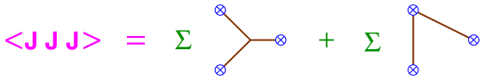
Figure 1: 3-point function at large $N_{C}$.

A simple diagrammatic analysis shows that at large $N_{C}$ the only singularities are one-meson poles.[WI:79] For instance, the two-point function takes the form: ⟨J(k)   J(-k)⟩= ∑_n f_n^2k2-Mn2   . Thus:

• $f_{n}=\langle 0|J|n\rangle\sim O(\sqrt{N_{C}}\,)$  and  $M_{n}\sim O(1)$.

• There are an infinite number of meson states, since $\langle J(k)\,J(-k)\rangle$ behaves logarithmically for large $k^{2}$.

• Mesons are free, stable and non-interacting.

At $N_{C}\to\infty$, the $n$-point functions are given by sums of tree diagrams with free meson propagators and effective local interaction vertices among $m$ mesons, which scale as  $V_{m}\sim O(N_{C}^{1-m/2})$. Moreover, $\langle 0|J|M_{1}\cdots M_{m}\rangle\sim O(N_{C}^{1-m/2})$. Each additional meson coupled to the current $J$ or to an interaction vertex brings then a suppression factor $1/\sqrt{N_{C}}$.

Including gauge-invariant gluon operators, such as $J_{G}=\mbox{\rm Tr}\left(G_{\mu\nu}G^{\mu\nu}\right)$, the diagrammatic analysis can be easily extended to glue states.[WI:79] Since $\langle T\left(J_{G_{1}}\cdots J_{G_{n}}\right)\rangle\sim O(N_{C}^{2})$, one derives the large–$N_{C}$ counting rules  $\langle 0|J_{G}|G_{1}\cdots G_{m}\rangle\sim O(N_{C}^{2-m})$  and  $V[G_{1},\cdots,G_{m}]\sim O(N_{C}^{2-m})$. Thus, at $N_{C}\to\infty$, glueballs are also free, stable, non-interacting and infinite in number. From the mixed correlators $\langle T\left(J_{1}\cdots J_{n}J_{G_{1}}\cdots J_{G_{m}}\right)\rangle\sim O(N_{C})$, one gets $V[M_{1},\cdots,M_{p};G_{1},\cdots,G_{q}]\sim O(N_{C}^{1-q-p/2})$. Therefore, glueballs and mesons decouple at large $N_{C}$, their mixing being suppressed by a factor $1/\sqrt{N_{C}}$.

Many known phenomenological features of the hadronic world are easily understood at lowest order in the $1/N_{C}$ expansion: suppression of the $\bar{q}q$ sea (exotics), quark model spectroscopy, Zweig’s rule, light SU(3) meson nonets, narrow resonances, multiparticle decays dominated by resonant two-body final states, etc. In some cases, the large–$N_{C}$ limit is in fact the only known theoretical explanation that is sufficiently general. Clearly, the expansion in powers of $1/N_{C}$ appears to be a sensible physical approximation at $N_{C}=3$.

The large–$N_{C}$ limit provides a weak coupling regime to perform quantitative QCD studies. At leading order in $1/N_{C}$, the scattering amplitudes are given by sums of tree diagrams with physical hadrons exchanged. Crossing and unitarity imply that this sum is the tree approximation to some local effective Lagrangian. Higher-order corrections correspond to hadronic loop diagrams.

2 Chiral Symmetry

With $n_{f}$ massless quark flavours, the QCD Lagrangian  [$\bar{q}=(\bar{u},\bar{d},\ldots)$] L_QCD^0 = -14  G^a_μν G^μν_a + i  ¯q_L^. γ^μD_μq_L^. + i  ¯q_R^. γ^μD_μq_R^. is invariant under global  $U(n_{f})_{L}\otimes U(n_{f})_{R}$ transformations of the left- and right-handed quarks in flavour space: $q_{L,R}^{\phantom{.}}\to g_{L,R}^{\phantom{.}}\;q_{L,R}^{\phantom{.}}\,$,   $g_{L,R}^{\phantom{.}}\in U(n_{f})_{L,R}^{\phantom{.}}\,$. Under very general assumptions it has been shown that, at $N_{C}\to\infty$, the symmetry group must spontaneously break down to the diagonal $U(n_{f})_{L+R}$.[CW:80] According to Goldstone’s theorem,[GO:61] $n_{f}^{2}$ pseudoscalar massless bosons appear in the theory, which for $n_{f}=3$ can be identified with the $U(3)$ multiplet

$$\Phi=\pmatrix{{1\over\sqrt{2}}\pi^{0}+{1\over\sqrt{6}}\eta_{8}+{1\over\sqrt{3}}\eta_{1}&\pi^{+}&K^{+}\cr\pi^{-}&-{1\over\sqrt{2}}\pi^{0}+{1\over\sqrt{6}}\eta_{8}+{1\over\sqrt{3}}\eta_{1}&K^{0}\cr K^{-}&\bar{K}^{0}&-{2\over\sqrt{6}}\eta_{8}+{1\over\sqrt{3}}\eta_{1}&}.$$

The unitary matrix U(ϕ) = u(ϕ)^2 = exp{i2Φ/f} gives a very convenient parameterization of the Goldstone fields. Under the chiral group it transforms as  $U(\phi)\to g_{R}^{\phantom{.}}\,U(\phi)\,g_{L}^{\dagger}$.

The Goldstone nature of the pseudoscalar mesons implies strong constraints on their interactions, which can be most easily analyzed on the basis of an effective Lagrangian.[WE:79] Since there is a mass gap separating the pseudoscalar nonet from the rest of the hadronic spectrum, we can build an effective field theory[EFT] (EFT) containing only the Goldstone modes. Moreover, the low-energy effective Lagrangian can be organized in terms of increasing powers of momenta (derivatives).

Let us consider an extended QCD Lagrangian, with quark couplings to external Hermitian matrix-valued fields $l_{\mu}$, $r_{\mu}$, $s$, $p$ : L_QCD = L^0_QCD + ¯q_L^. γ^μl_μ  q_L^. + q_R^. γ^μr_μ  q_R^. - ¯q_L^. (s - i p)  q_R^. - ¯q_R^. (s + i p)  q_L^.  . The external fields can be used to incorporate the electromagnetic and semileptonic weak interactions, and the explicit breaking of chiral symmetry through the quark masses: s = M+ …  ,     M= diag(m_u,m_d,m_s)   . At lowest order in derivatives and quark masses, the most general effective Lagrangian consistent with chiral symmetry has the form:[GL:85] L_2 = f^24  ⟨D_μU^†D^μU   +   U^†χ  +  χ^†U⟩  ,     χ≡2 B_0   (s + i p)   , where  $D_{\mu}U=\partial_{\mu}U-ir_{\mu}U+iU\,l_{\mu}$ , $\langle A\rangle$ denotes the flavour trace of the matrix $A$ and $B_{0}$ is a constant, which, like $f$, is not fixed by symmetry requirements alone. Taking functional derivatives with respect to the appropriate external fields, one finds that $f$ equals the pion decay constant (at lowest order) $f=f_{\pi}=92.4$ MeV, while $B_{0}$ is related to the quark condensate: B_0 = -⟨¯qq ⟩f2 = M_π^2mu+ md = M_K^0^2ms+ md = M_K^±^2ms+ mu  .

Formally, the chiral Lagrangian could be computed (non-perturbatively) from the QCD generating functional. The leading-order terms in $1/N_{C}$ should be of $O(N_{C})$, like the corresponding correlation functions of fermion bilinears. Moreover, they should have a single flavour trace since diagrams with $n$ quark loops have $n$ flavour traces and are of  $O(N_{C}^{2-n})$. The Lagrangian ${\cal L}_{2}$ obeys the correct $N_{C}$ counting rules: $f^{2}\sim O(N_{C})$, $B_{0}\sim M_{\phi}^{2}\sim U(\phi)\sim O(1)$. The $U(\phi)$ matrix generates an expansion in powers of $\phi/f$, giving the required $1/\sqrt{N_{C}}$ suppression for each additional meson field. Clearly, interaction vertices with $n$ mesons scale as $V_{n}\sim f^{2-n}\sim O(N_{C}^{1-n/2})$. Since ${\cal L}_{2}$ has an overall factor of $N_{C}$ and $U$ is $N_{C}$-independent, the $1/N_{C}$ expansion is equivalent to a semiclassical expansion. Quantum corrections computed with the chiral Lagrangian will have a $1/N_{C}$ suppression for each loop.

At $O(p^{4})$, the conventional $SU(3)_{L}\otimes SU(3)_{R}$-invariant chiral Lagrangian is usually written as:[GL:85]

$${\cal L}_{4} = L_{1}\,\langle D_{\mu}U^{\dagger}D^{\mu}U\rangle^{2}\,+\,L_{2}\,\langle D_{\mu}U^{\dagger}D_{\nu}U\rangle\,\langle D^{\mu}U^{\dagger}D^{\nu}U\rangle$$

$$\mbox{}+L_{3}\,\langle D_{\mu}U^{\dagger}D^{\mu}UD_{\nu}U^{\dagger}D^{\nu}U\rangle\,+\,L_{4}\,\langle D_{\mu}U^{\dagger}D^{\mu}U\rangle\,\langle U^{\dagger}\chi+\chi^{\dagger}U\rangle$$

$$\mbox{}+L_{5}\,\langle D_{\mu}U^{\dagger}D^{\mu}U\left(U^{\dagger}\chi+\chi^{\dagger}U\right)\rangle\,+\,L_{6}\,\langle U^{\dagger}\chi+\chi^{\dagger}U\rangle^{2}$$

$$\mbox{}+L_{7}\,\langle U^{\dagger}\chi-\chi^{\dagger}U\rangle^{2}\,+\,L_{8}\,\langle\chi^{\dagger}U\chi^{\dagger}U+U^{\dagger}\chi U^{\dagger}\chi\rangle$$

$$\mbox{}-iL_{9}\,\langle F_{R}^{\mu\nu}D_{\mu}UD_{\nu}U^{\dagger}+F_{L}^{\mu\nu}D_{\mu}U^{\dagger}D_{\nu}U\rangle\,+\,L_{10}\,\langle U^{\dagger}F_{R}^{\mu\nu}UF_{L\mu\nu}\rangle\,,$$

where $F^{\mu\nu}_{L,R}$ are field-strength tensors of the $l^{\mu}$ and $r^{\mu}$ flavour fields.

$i$	$L_{i}^{r}(M_{\rho})$	$O(N_{C})$	Source	$\Gamma_{i}$	$L_{i}^{N_{C}\to\infty}$
$2L_{1}-L_{2}$	$-0.6\pm 0.6$	$O(1)$	$K_{e4}$, $\pi\pi\to\pi\pi$	$3/16$	0
$L_{2}$	$\hphantom{-}1.4\pm 0.3$	$O(N_{C})$	$K_{e4}$, $\pi\pi\to\pi\pi$	$3/16$	$\phantom{-}1.8$
$L_{3}$	$-3.5\pm 1.1$	$O(N_{C})$	$K_{e4}$, $\pi\pi\to\pi\pi$	0	$-4.3$
$L_{4}$	$-0.3\pm 0.5$	$O(1)$	Zweig rule	$1/8$	0
$L_{5}$	$\hphantom{-}1.4\pm 0.5$	$O(N_{C})$	$F_{K}:F_{\pi}$	$3/8$	$\phantom{-}2.1$
$L_{6}$	$-0.2\pm 0.3$	$O(1)$	Zweig rule	$11/144$	0
$L_{7}$	$-0.4\pm 0.2$	$O(1)$	GMO, $L_{5}$, $L_{8}$	0	$-0.3$
$L_{8}$	$\hphantom{-}0.9\pm 0.3$	$O(N_{C})$	$M_{\phi}$, $L_{5}$	$5/48$	$\phantom{-}0.8$
$L_{9}$	$\hphantom{-}6.9\pm 0.7$	$O(N_{C})$	$\langle r^{2}\rangle^{\pi}_{V}$	$1/4$	$\phantom{-}7.1$
$L_{10}$	$-5.5\pm 0.7$	$O(N_{C})$	$\pi\to e\nu\gamma$	$-1/4$	$-5.4$

Table 1: Phenomenological values of the renormalized couplings $L_{i}^{r}(M_{\rho})$ in units of $10^{-3}$. The fourth column shows the source used to get this information. The large–$N_{C}$ predictions obtained within the single-resonance approximation are given in the last column.

Thus, at $O(p^{4})$ we need ten additional coupling constants $L_{i}$ to determine the low-energy behaviour of the Green functions. Terms with a single trace are of $O(N_{C})$, while those with two traces should be of $O(1)$. However, a $3\times 3$ matrix relation has been used to eliminate the additional structure $c\,\langle D_{\mu}U^{\dagger}D_{\nu}UD^{\mu}U^{\dagger}D^{\nu}U\rangle$ with the result $2\delta L_{1}=\delta L_{2}=-\frac{1}{2}\delta L_{3}=c\sim O(N_{C})$. As shown in Table 1, the phenomenologically determined values[EC:95, PI:95] of those couplings follow the pattern suggested by the $1/N_{C}$ counting rules. Moreover, their average order of magnitude, $L_{i}\sim f^{2}/(4\Lambda_{\chi}^{2})\sim 2\times 10^{-3}$, suggests a chiral symmetry-breaking scale $\Lambda_{\chi}\sim 1$ GeV.

One-loop graphs with the lowest-order Lagrangian ${\cal L}_{2}$ contribute also at $O(p^{4})$ in the chiral expansion, but they are suppressed by a factor of $1/N_{C}$. Their divergent parts are renormalized by the ${\cal L}_{4}$ couplings: L_i  =  L_i^r(μ)  +  Γ_i  μ^D-432 π2  { 2D-4 + γ_E - log(4π) - 1 } . This introduces a renormalization scale dependence, L_i^r(μ_2) = L_i^r(μ_1) + Γ_i(4π)2  log(μ_1μ2) , which is subleading in $1/N_{C}$. The phenomenological couplings given in Table 1 have been normalized at $\mu=M_{\rho}$.

The chiral loops generate non-polynomial contributions, with logarithms and threshold factors as required by unitarity, which are completely predicted as functions of $f$ and the Goldstone masses. Although they are suppressed by a factor of $1/N_{C}$, the chiral logarithms can be numerically important since $\frac{1}{N_{C}}\log{(\Lambda^{2}_{\chi}/M^{2}_{\pi})}\sim 4/3$.

2.1 Anomalies

Since chiral symmetry is explicitly violated by fermion anomalies at the fundamental QCD level,[AD:69] we need to add a functional $Z_{{\cal A}}$ with the property that its change under chiral transformations reproduces the anomalous change of the QCD generating functional. For the non-Abelian anomalies associated with the external sources $l_{\mu}$ and $r_{\mu}$, such a functional was first constructed by Wess and Zumino,[WZ:71] and reformulated in a nice geometrical way by Witten.[WI:83] It is an $O(p^{4})$ effect, which is completely calculable with no free parameters. This contribution is of  $O(N_{C})$, because it is generated by a triangle quark loop coupled to external sources.

Much more subtle is the $U(1)_{A}$ gluonic anomaly which breaks the conservation of the singlet axial quark current in the chiral limit: ∂_μ(¯qγ^μγ_5 q) = 2  n_f ω  ;   ω= α_s16π  ϵ^μνρσ  G_μν G_ρσ   . The corresponding anomalous change of the QCD generating functional can be accounted for by adding a term $\Delta{\cal L}_{\mathrm{QCD}}=-\theta\,\omega$ with the appropriate chiral transformation for the so-called vacuum angle $\theta(x)$.[KL:00] Notice that in the large–$N_{C}$ limit the $U(1)_{A}$ anomaly is absent.[WI:79b]

To lowest non-trivial order in $1/N_{C}$, the chiral symmetry breaking effect induced by the $U(1)_{A}$ anomaly can be taken into account in the effective low-energy theory, through the term[DVV:80] L_U(1)_A   =   - f^2 4 a NC   {θ- i2 [log(detU) - log(detU^†)] }^2 , which breaks $U(3)_{L}\otimes U(3)_{R}$ but preserves $SU(3)_{L}\otimes SU(3)_{R}\otimes U(1)_{V}$.

The parameter $\,a\,$ has dimensions of mass squared and, with the factor $1/N_{C}$ pulled out, is booked to be of $O(1)$ in the large–$N_{C}$ counting rules. Its value is not fixed by symmetry requirements alone; it depends crucially on the dynamics of instantons. In the presence of the term (2.1), the $\eta_{1}$ field becomes massive even in the chiral limit: M_η_1^2 = 3  aNC + O(M)   .

Owing to the large mass of the $\eta^{\prime}$, the effect of the $U(1)_{A}$ anomaly cannot be treated as a small perturbation. Rather, one should keep the term (2.1) together with the lowest-order Lagrangian (2). It is possible to build a consistent combined expansion in powers of momenta, quark masses and $1/N_{C}$, by counting the relative magnitude of these parameters as:[LE:96] O(p