Active-Sterile Neutrino Conversion: Consequences for the $r$-Process and Supernova Neutrino Detection

Abstract

We examine active-sterile neutrino conversion in the late time post-core-bounce supernova environment. By including the effect of feedback on the Mikheyev-Smirnov-Wolfenstein (MSW) conversion potential, we obtain a large range of neutrino mixing parameters which produce a favorable environment for the r-process. We look at the signature of this effect in the current generation of neutrino detectors now coming on line. We also investigate the impact of the neutrino-neutrino forward scattering-induced potential on the MSW conversion.

I Introduction

One form of element synthesis which may take place in core collapse supernovae (e.g., Type II, Ib, Ic) is the $r$-process, or rapid neutron capture process. The $r$-process of nucleosynthesis has long been thought to be the mechanism for producing many of the heavy nuclei (mass number, A $>$ 100) bbfh . Successful production of the r-process elements with anything approaching a solar system-like abundance distribution requires a neutron-rich environment, at least in the conditions suggested by current supernova models and simple neutrino-driven wind models without extremely rapid outflow and/or extremely relativistic neutron star configurations.

In this paper, we study a primary $r$-process which occurs in stages. The material in a fluid element moving away from the neutron star remnant left by a core collapse supernova explosion will experience three stages of nuclear evolution. First, only free nucleons are present, then alpha particles coexist with free neutrons. At still lower temperatures the matter is composed of alpha particles, “seed” nuclei with $50\lesssim A\lesssim 100$, and neutrons. In the last stage the neutrons capture on the seed nuclei.

The neutrino-driven-wind environment, which is thought to occur at late time (time post bounce $t_{pb}\sim 10{\rm s}$) in the supernova is a promising candidate site for the production of the r-process elements r1 . The wind is thought to arise well after the initial collapse/explosion event; its successful generation of course presupposes a successful explosion. In the classic neutrino driven wind models, neutrinos transfer energy to material near the surface of the protoneutron star. As this material flows outward, it expands and cools. As it cools, weak and electromagnetic/strong nuclear reaction rates drop out of equilibrium sequentially. If enough neutrons are present after/during this freeze-out process, the $r$-process may take place. The number of neutrons is determined by three factors, the initial neutron-to-proton ratio, the outflow timescale and the entropy of the material. Semianalytic models of the neutrino driven wind have shown that it is difficult, though perhaps not impossible, to generate the required numbers of neutrons per seed nucleus hwq .

Self-consistent inclusion of neutrino capture reactions into a reaction network code has shown that the problem of obtaining the required number of neutrons is exacerbated by the interplay between neutrino and nuclear reactions, especially the formation of alpha particles as described below mmf . This is the so-called “alpha effect.” The relative number of neutrons and protons is usually cast in terms of the electron fraction, $Y_{e}=1/(1+n/p)$, the net number of electrons (electrons minus positrons) per baryon. The electron fraction is determined mostly by the rates of neutrino and antineutrino capture on free neutrons and protons Qetal . The most detrimental effect, the alpha effect, takes place when material which would eventually undergo heavy element nucleosynthesis passes through the intermediate step of forming alpha particles. At this stage, all the protons are locked into alphas, but any excess neutrons remain free. Neutrino captures on the remaining neutrons decrease the ratio of neutrons to protons (or equivalently raise the electron fraction). Supernova neutrino energies are too low to permit compensating charged current captures on alpha particles mmf . Without sufficient numbers of neutrons, there can be no rapid neutron capture process in these sorts of wind scenarios.

There are three potential solutions to this problem. One solution involves hydrodynamics. For example, a very fast outflow may in principle cure the problems associated with this environment hwq and also the alpha effect cf . Alternately, other scenarios which have rapid expansion (perhaps followed by a slow down) accompanied by high entropy and temperature may also cure the problem r1 . However, it is not clear that such a fast outflow or high entropy is present in this environment, or that either can be achieved with simple neutrino heating.

The second solution may be to look for another site, such as neutron star mergers. Some neutron rich material may be ejected in the merger and this has been shown to be capable of producing r-process elements bsm89 . These mergers are likely too rare to reproduce the total observed abundance of r-process elements, unless a significant fraction of the neutron star material is ejected thielemann . There is significant energy released in the form of neutrinos in these models. Therefore, the alpha effect may compromise the r-process in these environments as well, although the neutrino average energies in neutron star -neutron star mergers could be somewhat lower than in core collapse supernovae and neutron star - black hole mergers, as discussed in e. g. Ref. janka99 .

A third solution is the one that is investigated in this paper: active-sterile ($\nu_{e}\leftrightarrow\nu_{s}$, $\bar{\nu_{e}}\leftrightarrow\bar{\nu_{s}}$) neutrino transformation. The $\nu_{s}$ in our study is defined as a particle which mixes with the $\nu_{e}$ (and possibly also with $\nu_{\mu}$, and/or $\nu_{\tau}$) but does not contribute to the width of the Z boson. One candidate for this particle, although not the only one, is a right handed Dirac neutrino. A large number of models exist for such light “sterile” neutrinos, for example, any SU(2) Standard Model singlet.

In fact, the existence of sterile neutrinos with large masses (e.g., of order the unification scale) would not be unexpected, as they are suggested by many neutrino mass/mixing models. However, light sterile neutrinos do not often occur naturally in these models.

The Sudbury Neutrino Observatory (SNO) and the SuperKamiokande (SuperK) experiments together observe high energy solar neutrinos and SuperK can observe and characterize the atmospheric neutrino flux. What is emerging is a picture in which there is near maximal mixing between the mu and tau flavor neutrinos at the atmospheric neutrino mass-squared difference scale $\delta m^{2}\approx 3\times{10}^{-3}\,{\rm eV}^{2}$, and a convincing result that two-thirds of the neutrinos coming from the sun are mu/tau neutrinos, narrowly favoring again near maximal mixing between the electron flavor neutrinos produced by nuclear reactions in the sun and mu/tau flavor neutrinos at the solar neutrino mass-squared difference $\delta m^{2}<{10}^{-4}\,{\rm eV}^{2}$ superk ; sno ; bah . Is there any indication of light sterile degrees of freedom?

The Los Alamos Liquid Scintillator Neutrino Detector (LSND) experiment remains the only possible indication of neutrino flavor oscillations (in the $\nu_{\mu}\rightleftharpoons\nu_{e}$ channel at a neutrino mass-squared scale $\delta m^{2}\sim 0.5\,{\rm eV}^{2}$) beyond those derived from solar and atmospheric neutrino considerations lsnd . The mini-BooNE experiment at Fermilab will soon check this result. If LSND holds up then it is tantamount to direct evidence for the existence of a light sterile neutrino. Four neutrino schemes designed to fit all of the existing neutrino oscillation data gg are, however, barely viable or are outright challenged by the data. By contrast, we emphasize here that our considerations of the effect of a sterile neutrino on supernova physics are completely independent of the LSND result. For example, the sterile neutrino mass range which we find to be efficacious in supernova r-process nucleosynthesis spans the entire LSND-inspired range but also extends to considerably higher values of $\delta m^{2}$ and to smaller vacuum mixing angles.

The effect of active-sterile transformation differs from that of active-active (e.g., $\nu_{e}\leftrightarrow\nu_{\mu\tau}$) transformation, in that active-active transformation usually tends to decrease the number of neutrons in the supernova, while active-sterile transformation can increase it. (Active-active transformation can slightly decrease the electron fraction for certain narrow ranges of neutrino mass-squared difference.) It has been shown that matter-enhanced $\nu_{e}\leftrightarrow\nu_{\mu,\tau}$ could under some circumstances rather drastically affect the neutron to proton ratio in the neutrino-driven wind and, thereby, affect the prospects for the r-process there Qetal .

Active-sterile transformation in the supernova environment must be treated carefully for several reasons. The first is that, due to the structure of the Mikheyev-Smirnov-Wolfenstein (MSW) conversion potential, both neutrinos and antineutrinos may undergo transformation in the same scenario. In fact, in the solutions discussed here both types of transformations take place. The second is that the neutrinos themselves in part determine the MSW potential. Any calculation of the effect of oscillations must therefore include a feedback loop. The neutrinos determine the electron fraction; the electron fraction determines the potential; and the potential determines the spectrum of neutrinos. The spectrum of neutrinos then sets the electron fraction. Additionally, the $\nu\nu$-forward scattering contribution to the MSW potential depends on the flavor states of the neutrinos.

In section II we review the calculations which illustrate the feedback mechanism us . Our study differs from a previous study nunokawa in that we track the thermodynamic and nuclear statistical equilibrium evolution (NSE) of a mass element and update the numbers of neutrons and protons at each time step directly from the weak capture rates. This is essential to accurately determine the number of neutrons available for the r-process. In addition to producing a favorable $n/p$ ratio, this type of transformation can suppress the population of $\nu_{e}$ and thereby defeat the alpha effect. In section III we discuss the observational consequences of such a neutrino flavor transformation scenario in current neutrino detectors. In section IV we explore the importance of neutrino background terms, or neutrino-neutrino scattering in the MSW potential. In section V we give conclusions.

II The Mechanism

In this section, we briefly describe our calculations and then we summarize the impact of active-sterile neutrino transformation on the electron fraction in the neutrino driven wind. Our study in this paper differs from that in our earlier work in Ref. us in that here we discuss the expected effects of active-sterile neutrino flavor transformation on the expected supernova neutrino signal in several different detectors and we also consider effects of the neutrino-neutrino forward scattering-induced potential (the “neutrino background”) on the neutrino flavor transformation problem.

If we neglect $\nu$-$\nu$ forward scattering contributions to the weak potentials, then the equation which governs the evolution of the neutrinos as they pass though the material in the wind can be written as:

$$i\hbar\frac{\partial}{\partial r}\left[\begin{array}[]{cc}\Psi_{e}(r)\\ \\ \Psi_{s}(r)\end{array}\right]=\left[\begin{array}[]{cc}\varphi_{e}(r)&\sqrt{\Lambda}\\ \\ \sqrt{\Lambda}&-\varphi_{e}(r)\end{array}\right]\left[\begin{array}[]{cc}\Psi_{e}(r)\\ \\ \Psi_{s}(r)\end{array}\right]\,,$$ (1)

where

$$\varphi_{e}(r)=\frac{1}{4E}\left(\pm 2\sqrt{2}\ G_{F}\left[N_{e}^{-}(r)-N_{e}^{+}(r)-\frac{N_{n}(r)}{2}\right]E-\delta m^{2}\cos{2\theta_{v}}\right)$$ (2)

The upper sign is relevant for neutrino transformations; the lower one is for antineutrinos. In these equations

$$\sqrt{\Lambda}=\frac{\delta m^{2}}{4E}\sin{2\theta_{v}},$$ (3)

$\delta m^{2}\equiv m_{2}^{2}-m_{1}^{2}$ is the vacuum mass-squared splitting, $\theta_{v}$ is the vacuum mixing angle, $G_{F}$ is the Fermi constant, and $N_{e}^{-}(r)$, $N_{e}^{+}(r)$, and $N_{n}(r)$ are the total proper number densities of electrons, positrons, and neutrons respectively in the medium. Again, this form of the potential, $\varphi_{e}(r)$, is valid only in the absence of neutrino background effects. The background effects will be explored in detail in Section IV, but we note that Eq. (1) is adequate for following $\nu$ flavor evolution well above the neutron star.

Eq. (2) can be rewritten in terms of a potential,

$$V(r)=2\sqrt{2}G_{F}\left[N_{e}^{-}(r)-N_{e}^{+}(r)-\frac{N_{n}(r)}{2}\right].$$ (4)

Then the on-diagonal term in the Hamiltonian becomes

$$\varphi_{e}(r)=\frac{1}{4E}\left(\pm V(r)E-\delta m^{2}\cos 2\theta_{v}\right).$$ (5)

Neutrinos undergo a resonance and transform primarily when the on-diagonal term is zero, that is, at the resonant energy

$$E_{res}(r)=\pm\frac{\delta m^{2}\cos 2\theta_{v}}{V(r)}.$$ (6)

We see that neutrinos undergo resonance when the potential is positive, and antineutrinos undergo resonance when it is negative. Finally, we rewrite the potential in terms of the electron fraction,

$$V(r)=\frac{3G_{F}\rho(r)}{2\sqrt{2}m_{N}}\left(Y_{e}-\frac{1}{3}\right),$$ (7)

where

$$Y_{e}(r)=\frac{N_{e}^{-}(r)-N_{e}^{+}(r)}{N_{p}(r)+N_{n}(r)}.$$ (8)

Here $\rho(r)$ is the density of the matter at distance $r$ from the protoneutron star, and $m_{N}$ is the mass of a nucleon and $N_{p}(r)$ is the total proper proton number density. We assume that $N_{p}=N_{e}^{-}-N_{e}^{+}$ because of local electromagnetic charge neutrality. Since the electron fraction can take on values between zero and one, the potential can be either positive or negative. Therefore, depending on the value of the electron fraction, either neutrino or antineutrino transformation may be matter-enhanced.

We solve Eq. (1) numerically for survival probabilities of neutrinos as they pass through the matter above the protoneutron star. No approximations are employed in computing the survival probabilities, for the adopted potential. In the absence of oscillations and matter-enhanced flavor transformation, the spectrum of neutrinos and antineutrinos can be parameterized as approximately Fermi-Dirac in character. We assume that no transformation has taken place within the protoneutron star, so we begin with a full complement of each species of active neutrino. However, since neutrinos of different energies will have different survival probabilities at each distance above the surface, the distribution quickly departs from the Fermi-Dirac shape. We use representative initial neutrino distributions with temperatures of ${\rm T}_{\nu_{e}}=3.22\,{\rm MeV}$ and ${\rm T}_{\bar{\nu}_{e}}=4.5\,{\rm MeV}$, luminosities of $L_{\nu_{e}}=1.08\times 10^{51}{\rm ergs}\,{\rm s}^{-1}$ and $L_{\bar{\nu}_{e}}=1.3\times 10^{51}{\rm ergs}\,{\rm s}^{-1}$ and effective chemical potentials of zero. Though different numerical simulations of neutrino transport in the hot protoneutron star core differ in their predictions of these spectral values, we note that our adopted values serve to illustrate the general qualitative behavior that would be expected if the simulations included this neutrino flavor transformation physics.

In the neutrino driven wind, the neutrinos and antineutrinos are the most important agents in determining the electron fraction. However, near the surface of the protoneutron star there is also a contribution from electrons and positrons:

$$\nu_{e}+{\rm n}\rightleftharpoons{\rm p}+e^{-};$$ (9)

$$\bar{\nu}_{e}+{\rm p}\rightleftharpoons{\rm n}+e^{+}.$$ (10)

Close to the surface of the protoneutron star, these weak capture rates are fast in comparison with the outflow timescale. As we move far from the surface, they become negligible in comparison with outflow. Therefore the weak capture rates are in the process of freezing out of steady state (chemical) equilibrium. We calculate the electron fraction by numerically following the evolution of the number densities of neutrons and protons.

Our calculations are performed by tracking the evolution of mass elements in the neutrino driven wind. We use distance and density profiles from analytic descriptions of the wind; $r\propto\exp(-t/\tau)$ and $\rho\propto r^{-3}$ where $\tau$ is the outflow timescale qw . For illustrative purposes, we use a timescale of $\tau=0.3\,{\rm s}$ and an entropy per baryon of $s=100$ in units of Boltzmann’s constant. Close to the surface of the protoneutron star, before the wind begins to operate, we use the density profile of Wilson and Mayle wilson . Calculations done with different timescales show the same qualitative features that we present here us and variations in the entropy are expected to have a similar effect.

At each time step the distance and density are incremented. All other thermodynamic quantities, including the number densities of positrons and electrons, are calculated from the entropy and density. The mass fractions of the neutrons, protons, alpha particles and heavy nuclei (A $>$ 40) are calculated in NSE (Nuclear Statistical Equilibrium). The weak rates are then computed and the electron fraction is updated. This new electron fraction is used in the MSW equations to calculate new survival probabilities for each neutrino energy bin. We terminate calculations for a particular mass element at the point when heavy nuclei begin to form. Since the outflow times considered in our calculations are relatively short, $t\sim\tau\lesssim 0.5\,{\rm s}$, we have assumed that each mass element experiences the same evolution as the previous ones.

The consequences of the feedback effect are illustrated in Figure 1. In this figure, the electron fraction is plotted against distance as measured from the center of the protoneutron star. The upper curve shows the evolution of the electron fraction in the absence of neutrino transformation, while the lower curve shows the evolution of the electron fraction for mixing parameters of $\delta m^{2}=20\,{\rm eV}^{2}$, $\sin^{2}2\theta_{v}=0.01$. The initial rise in the electron fraction is due to Pauli unblocking of neutrino capture on neutrons as the density rapidly decreases at the edge of the protoneutron star. At such high density we do not include feedback effects; the validity of this approximation is discussed below. We begin the feedback effects at about the distance where the wind solution begins to dominate the hydrodynamic flow. In the case of no transformation the electron fraction shows a slight drop, due to the decreasing importance of electron and positron capture, and then a slight rise due to the alpha effect.

In the presence of mixing, however, the situation is quite different. Low energy electron neutrinos begin to transform slightly above the surface of the protoneutron star, where the potential is large (Eq. 6). This transformation decreases the rate of neutrino capture on neutrons, which lowers the electron fraction, and therefore the potential. Thus neutrinos of higher and higher energy begin to transform. Eventually the electron fraction drops below 1/3, so the potential becomes negative, and the highest energy electron antineutrinos begin to transform. This slows down the drop in $Y_{e}$, but does not halt it entirely, since low energy electron antineutrinos are still present. As the electron fraction continues to fall, the magnitude of $V$ increases, so lower energy electron antineutrinos transform. Meanwhile, the mass density is falling, causing the potential to reach a minimum and, eventually, return toward zero. The minimum means that only antineutrinos above a certain energy will undergo resonance, and since the potential goes back to zero, all these neutrinos (originally active antineutrinos) are re-converted from sterile to active species. By the time alpha particles form, there are many electron antineutrinos present but few electron neutrinos. Therefore, there is no alpha effect. The resulting electron fraction is so low $\sim 0.1$, that conditions become favorable for the r-process. There is no alpha effect because the $\nu_{e}$’s that would have captured on neutrons during the epoch of alpha particle formation are, for the right neutrino mass/mixing parameters, converted to sterile species in large measure at the alpha formation epoch. A study of many different neutrino driven wind conditions, shows that for a timescale of 0.3 s and an entropy per baryon of $\sim 100$, the electron fraction must be below 0.18 in order to produce the requisite neutron to seed ratio meyer97 .

An analysis in Ref. nunokawa assumed that $Y_{e}(r)$ was equal to its equilibrium value, as set from the weak capture rates (us, , Eq. 3.14). Ref. nunokawa neglected electron and positron capture in finding the equilibrium value of of $Y_{e}(r)$, and did not take into account alpha particle formation and did not take account of the feedback of the outflow rate on neutrino capture processes and neutrino flavor transformation. Similarly, Ref. peres did not include this physics. Without these effects, the system finds a fixed point at $Y_{e}=1/3$; neutrino conversions bring the electron fraction to this value. Once there, the neutrino-matter forward scattering-induced potentials vanish and there is no further neutrino flavor transformation in the channels $\nu_{e}\rightleftharpoons\nu_{s}$ and $\bar{\nu}_{e}\rightleftharpoons\bar{\nu}_{s}$. In Fig. 2, we have duplicated this result by making the assumptions outlined above. The figure also shows the evolution of $Y_{e}$ when we take account of alpha formation, but keep the other simplifications as above. In this case, $Y_{e}$ goes to 1/3 as before, but then the alpha effect drives it to 1/2 eventually. These results hold for a broad range of neutrino mixing parameters.

Except in Fig. 2 we have carefully tracked the actual value of $Y_{e}$ as distinct from its equilibrium value; we have also taken account of electron and positron captures and alpha formation. In this case, $Y_{e}$ lags behind its equilibrium value. As a result, $Y_{e}$ remains greater than 1/3, even when the equilibrium electron fraction ${(Y_{e})}_{\rm eq}$ drops below that value. Therefore, neutrinos continue to transform, and eventually drive the system to low electron fraction values, $Y_{e}<1/3$.

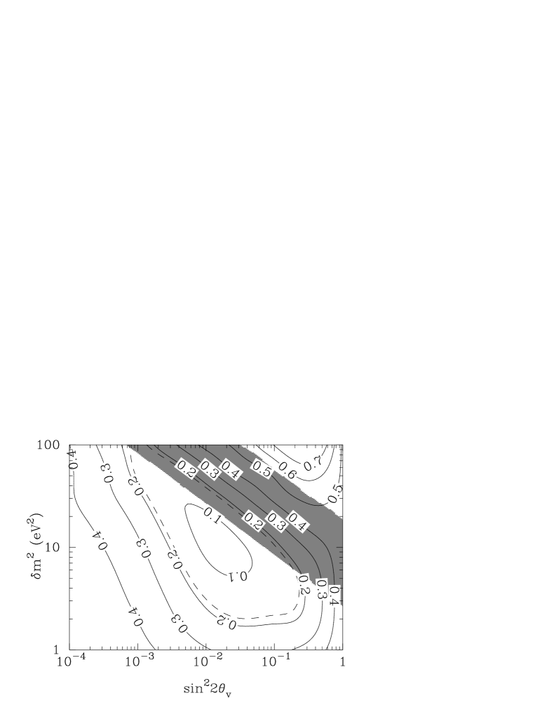
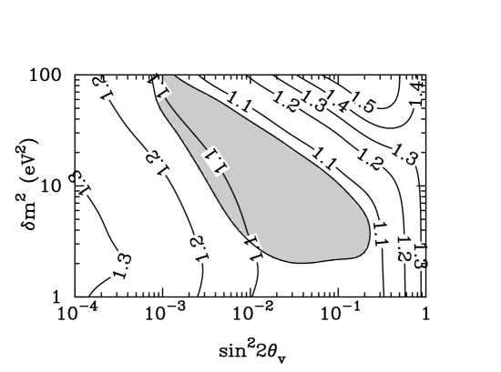
We investigate a range of mixing parameters in Figure 3. This contour plot shows the electron fraction, measured at the point where heavy nuclei begin to form, for various mixing parameters. Here we employ the same neutrino driven wind model used in Figure 1. In the bottom left corner of the plot, the solution is approaching the case without neutrino transformation. In the middle of the plot, the transformations of neutrinos produce a very neutron rich environment.

In the upper right part of the plot, the electron neutrinos are undergoing an additional resonance, at smaller distance than those described above, and in fact close to the neutron star surface where the density scale height is small. This resonance occurs at the first place where the electron fraction passes close to 1/3, at very high density. To correctly model this range of mixing parameters it is necessary to include feedback in the very dense region near the neutron star surface.

In addition, because this resonance is so close to the neutrinosphere, some neutrinos travel through it along extremely nonradial paths. In general neutrinos which travel nonradially transform differently from those which travel radially, but for most of our parameter space, the effects are small. The results presented here include only radial paths. We have checked them against another (very slow) calculation, which includes nonradial effects. The difference is negligible except when neutrinos or antineutrinos transform at this inmost resonance.

We have drawn a shaded area on the contour plot. In this shaded area the inclusion of nonradial neutrino paths would alter the results by more than 10%. We show this also in Fig. 4. Here the difference in survival probabilities of electron neutrinos at 11 km is plotted. The same wind parameters are used here as in Fig. 3.

This shaded region of Fig. 3 (and also the unshaded region in the upper right corner above it) would also require us to take account of feedback effects in the steep density gradient region near the neutrino sphere. We have not included a full nonradial calculation of the results there. These regions of the plot require further investigation before definitive conclusions about the evolution of the electron fraction can be drawn. The work of Ref. mitesh has discussed the difficulties inherent in treating the steep region. We emphasize, however, that the rest of our parameter space presents a favorable environment for the $r$-process.

III Detection

In this section we study the supernova neutrino signal that would be seen at SNO or SuperKamiokande after active-sterile transformation. We consider the $\nu_{e}$, and $\bar{\nu}_{e}$ parameters used in section II and additional individual neutrino parameters of $T_{\nu_{\mu},\bar{\nu}_{\mu},\nu_{\tau},\bar{\nu}_{\tau}}=6\,{\rm MeV}$ and $L_{\nu_{\mu},\bar{\nu}_{\mu},\nu_{\tau},\bar{\nu}_{\tau}}=1\times 10^{51}{\rm ergs}\,{\rm s}^{-1}$ .

A galactic supernova is expected to produce a large electron antineutrino signal in SuperK. In fact, a supernova at 10 kiloparsecs is estimated to see about 8000 events from $\nu_{e}+n\rightarrow e^{-}+p$ superK . In principle, there will be an additional 300 events from neutrino scattering on electrons. Since both charged and neutral current processes contribute to this type of scattering, all types of neutrinos, except sterile will contribute.

SNO will see an estimated 500 events from neutral current break-up of the deuteron, $\nu_{x}+d\rightarrow n+p$ and an additional 150 for each of the charged current processes, $\nu_{e}+d\rightarrow p+p+e^{-}$ and $\bar{\nu}_{e}+d\rightarrow n+n+e^{-}$ SNO . These break-up reactions may be distinguished and tagged by the presence or absence of the emitted neutron(s) and the Cerenkov light from the electron or positron.

III.1 Active-sterile transformation alone

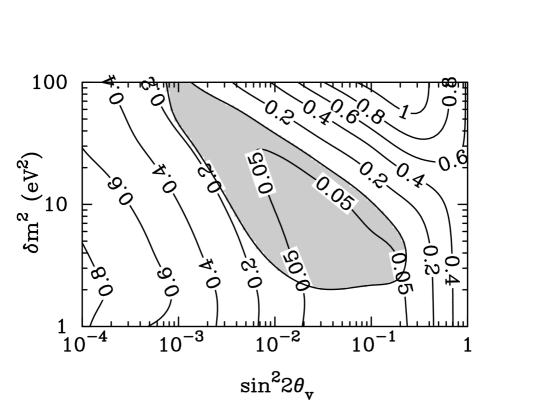
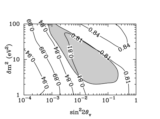
Figure 5 shows the ratio of the expected charged current electron neutrino-induced event rates in SNO for the case with active-sterile transformation to the case without such transformation. In the region which produced the lowest electron fraction in Figure 3, we find that the charged current event rate is suppressed by 90%. In the lower left hand corner of the plot, the ratio approaches one as the solution asymptotes to the case of no transformation. In Figs. 5 - 8, the shaded region shows where the neutron to seed ratio should be greater than 100 (i.e. favorable for the r-process) for the given wind parameters.

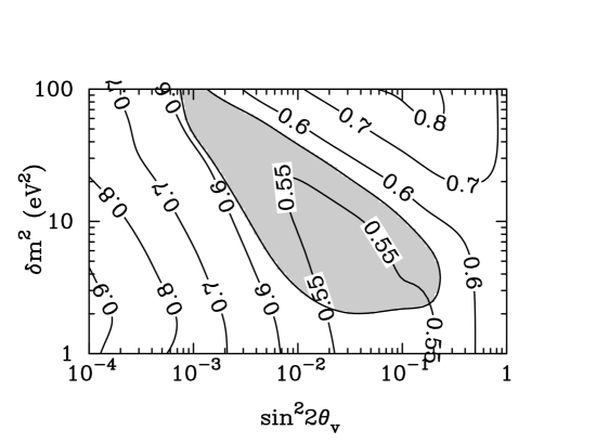
Figure 6 shows the ratio of the expected electron neutrino-induced scattering events from all processes at Superkamiokande for the case with active-sterile transformation to the case without such transformation. Because the charged current electron neutrino scattering rate is so much larger than the neutral current one, the absence of electron neutrinos has a significant $\sim 40$% effect. This may be surprising since the $\nu_{\mu}$,$\bar{\nu}_{\mu}$,$\nu_{\tau}$, and $\bar{\nu}_{\tau}$ have two and a half times the energy of the $\nu_{e}$ on average and the cross section is approximately linear in neutrino energy. However, the luminosities of the species are roughly the same, so the number flux of the high energy neutrinos is two and half times less than the number flux of the lower energy neutrinos. Therefore most of the small energy dependence in the rate stems from the 5 MeV detection threshold in SuperK.

These figures demonstrate that because of the deficit of electron neutrinos produced by the active-sterile solution, the SNO charged current rate will be greatly reduced from the expected event rate. However, the SuperK electron (antineutrino) capture rate will be for the most part unchanged. Note that our model is, therefore, unconstrained by data from supernova 1987A.

The calculations of detector signals have assumed no other type of neutrino mixing until this point. However, both the atmospheric neutrino mixing solution and the solar neutrino solution will cause additional oscillations. The effect of $3\,\times\,3$ active only mixing on a supernova neutrino signal has been discussed in the literature (ref. fhm ; dighe ). The vacuum mixing of $\nu_{\mu}\leftrightarrow\nu_{\tau}$ which may solve the atmospheric neutrino problem will cause $\nu_{\mu}\leftrightarrow\nu_{\tau}$ mixing in supernova neutrinos. Since the $\nu_{\mu}$ neutrinos and the $\nu_{\tau}$ neutrinos have the same energies and luminosities, this mixing will not directly cause changes in the detector signal. In the following discussion, we assume $\sin^{2}2\theta_{atm}\approx\sin^{2}2\theta_{23}=1$.

III.2 SMA and active-sterile transformation

We also consider the situation where $\nu_{e}\leftrightarrow\nu_{\mu}$ MSW is the solution to the solar neutrino problem. The small mixing angle (SMA) parameters, $\delta m^{2}_{solar}=5\times 10^{-6}\,{\rm eV}^{2}$ and $\sin^{2}2\theta_{solar}=\sin^{2}2\theta_{12}\approx 10^{-2}$ will cause partial conversion in the hydrogen envelope of the supernova progenitor star. The exact survival probabilities will depend on the electron density scale height:

$$R_{s}=-{N_{e}\over dN_{e}/dr}.$$ (11)

We use densities and distances from Ref. woosley to estimate $R_{s}\approx 10^{10}{\rm cm}$. We assume here that the density and composition will be largely unaffected by the core collapse event at the time that the neutrinos move through it. For 30 MeV neutrinos, near-total conversion (electron neutrino survival probability less than 1%) requires the density profile to be much shallower: $R_{s}>8\times 10^{10}$ cm. For no conversion (electron neutrino survival probability more than 99%), the density profile must be much steeper: $R_{s}<1\times 10^{8}$ cm. Therefore it is very likely that partial conversion of the electron neutrinos will take place, even given a more detailed model of the hydrogen envelope.

Using a fit to the points given in ref. woosley , we obtain ratios for the SNO charged current electron neutrino scattering rate (Figure 7) and the SuperK electron neutrino rate (Figure 8), with both the active-sterile mixing and the additional envelope conversion. Again, we show results in terms of ratios: the expected detector supernova neutrino-induced event rates with two types of mixing to the expected event rates in the case with no neutrino flavor conversion. The SuperK electron antineutrino capture rate is the same as in Figure 4, since no electron antineutrino conversion occurs in the envelope.

Figure 7 shows that the partial conversion of muon neutrinos to electron neutrinos, after the initial conversion of electron neutrinos to steriles, produces a ratio of order one. Figure 8 shows that electron scattering ratio of rates at SuperK with conversion. The partial conversion of the muon neutrinos more or less reproduces the case with no transformation whatsoever.

III.3 LMA and active sterile transformation

In table 1 we show a few of the possible outcomes for final electron neutrino spectrum, as a result of the active-active mixings. The relevant parameters are $\theta_{12}$, $\theta_{13}$ and the associated $\delta m^{2}$s. The case of maximal mixing for the atmospheric neutrinos and the large angle solution to the solar neutrino problem, with $\sin^{2}2\theta_{12}\approx\sin^{2}2\theta_{solar}\sim 0.8$ is shown. Here we implicitly assume a normal (as opposed to an inverted) neutrino mass hierarchy.

As in the case of small angle mixing, the Large Mixing Angle (LMA) solar parameters will cause neutrino flavor conversion in the supernova at a density comparable to where resonant neutrino flavor conversion takes place in the sun. In the supernova progenitor, this resonance will be located in the helium/hydrogen envelope for typical neutrino energies. If the supernova progenitor density profile is fairly smooth, then there will likely be an adiabatic level crossing at this location, so that the $\nu_{e}$ will wind up with an energy spectrum which would be measured as $\sin^{2}\theta_{solar}$ of the original $\nu_{e}$ spectrum and $\cos^{2}\theta_{solar}$ of the originally “hotter” $\nu_{\mu}$ and $\nu_{\tau}$ type spectrum. The “hopping probability” at resonance will be much smaller for the large angle solution than in the case of the SMA. For the LMA solution, even if the resonance is completely nonadiabatic so that there is no level crossing at resonance, the electron neutrinos will still become more energetic on account of their large vacuum mixing with mu and tau neutrinos.

With the LMA included, the difference between the active-sterile neutrino conversion case considered here and the case with no steriles is that part of the $\nu_{e}$ spectrum simply disappears at some point during the deleptonization “cooling” epoch of the proto-neutron star. At early times, when the density profile is too steep for much active-sterile transformation to occur, the “cold” part (or the part that was originally $\nu_{e}$) of the spectrum will be present, and at late times, when the transformation begins and the r-process takes place, this part will disappear. We show this pictorially in Fig. 9.

In Fig. 9 the bottom panel shows what happens to the neutrino spectrum if $\nu_{e}\leftrightarrow\nu_{s}$ resonant neutrino flavor conversion is significant and no subsequent vacuum mixing or envelope conversion takes place. The solid curve corresponds to the early time, when the density profile is too steep for much flavor transformation to occur and the dashed curve corresponds to the late time when the evolution is adiabatic.

The top panel of Fig. 9 shows the case where the LMA parameters provide the solution to the solar neutrino problem. We assume completely adiabatic transformation in the supernova progenitor envelope in this case. In this panel, the original $\nu_{e}$ spectrum becomes mixed with the $\nu_{\mu}$ and $\nu_{\tau}$, through the solar parameters $\sin^{2}2\theta_{solar}\approx 0.8$. This is evident in the figure: note, for example, the longer tail on the distribution function. The early time (solid line) case, where the $\nu_{e}\leftrightarrow\nu_{s}$ transformation is inoperative, has many more counts at low energy than does the late time scenario. From this curve it is evident that measuring the low energy part of the neutrino spectrum would be most useful for determining whether large scale active-sterile transformation occurs. A dramatic change in the number of low energy neutrinos relative to the number of high energy neutrinos would be an indication that the type of active-sterile transformation discussed here was taking place.

III.4 The third active-active mixing angle

An interesting case occurs if the unknown parameters $\theta_{13}$ and $\delta m_{13}^{2}$ are such that a second resonance occurs at a density between the $\nu_{e}\leftrightarrow\nu_{s}$ transformation density and the resonance region associated with $\delta m^{2}_{12}$. In the case of complete neutrino flavor transformation, the $\nu_{e}$’s are almost completely transformed into $\nu_{\mu,\tau}$ and vice versa. In this case, neutrinos which were originally electron flavor when they left the neutrino sphere are almost completely coincident with the $\nu_{3}$ state. This state evolves separately and does not encounter subsequent mixing with the other flavors bf ; cfq . In this special case of complete transformation at the $\delta m^{2}_{13}$ resonance, it would be more difficult to recognize the effects of a $\nu_{e}\leftrightarrow\nu_{s}$ transformation at a higher density.

III.5 Detection Summary

If only active-sterile transformation takes place, there would be a dramatic deficit in the expected charged current signal in SNO. However, with $\nu_{e}\leftrightarrow\nu_{\mu,\tau}$ transformations included as well, whether the detected signal is distinguishable from the case with no steriles depends on the oscillation parameters and the density and electron fraction profiles in the supernova. One signal of the active-sterile mixing and the LMA would be a decrease in the number of low energy neutrinos with time.

We note that we have not considered in this section the mixing of the sterile neutrino with the other (mu and tau) active neutrino species. Such mixing opens a large new range of parameter space. Depend on the $\delta m^{2}$s and mixing angles, this additional unknown mixing could alter the results presented in this section. Finally, density fluctuations, both near the protoneutron star and in the progenitor envelope may also change these results loreti .

IV Background

In this section we consider the effects of the neutrino background potential. The neutrino-neutrino forward scattering-induced “background” potential adds an important new twist to resonant neutrino flavor conversion, rendering the problem severely nonlinear. This potential can be written

$$V_{\nu}=2\sqrt{2}G_{F}N_{\nu}.$$ (12)

Here $N_{\nu}$ is the effective (because a neutrino’s individual contribution depends on the angle it makes with the “test” neutrino) net (neutrinos minus antineutrinos) neutrino number density. In the case of active-sterile mixing, only the flavor basis on-diagonal terms entering into Eq. (1) are non-vanishing, although in the general case of active-active mixing, both on- and off-diagonal matrix elements of the neutrino-neutrino forward scattering potential in the flavor basis could be nonzero pantaleone:offd ; sigl-raffelt:kinetic . We only need to take account of electron neutrinos forward-scattering on active flavors, since we assume that the matrix elements for electron neutrinos to forward-scatter off steriles are negligible, as are the matrix elements for sterile neutrino forward-scattering off other sterile species sigl-raffelt:kinetic . See Ref. qf:background for a discussion of the background effect in active-active neutrino mixing.

The effective neutrino number density is written as

$$N_{\nu}=\int d^{3}q\left(1-{p\cdot q\over|p||q|}\right)(\rho_{q,aa}-\bar{\rho}_{q,aa}).$$ (13)

Here $q$ is the momentum of the background neutrino, $p$ is the momentum of the test neutrino, $\rho_{q,aa}$ is the density matrix element for neutrino-neutrino forward scattering and $\bar{\rho}_{q,aa}$ is the corresponding density matrix element for the antineutrinos. In these expressions for the density matrix elements, the subscript $aa$ denotes the flavor-diagonal matrix element, so that $a=e$,$s$, electron or sterile flavor, respectively. We write the density matrix elements as

$$\rho_{q,aa}=N(r,R_{\nu},E_{q})P(r,E_{q},\psi)$$ (14)

where $E_{q}$ is the energy of a neutrino with momentum $q$. $N(r,R_{\nu},E_{q})$ is the number density of neutrinos emitted into a pencil of direction and energy interval $d^{3}q$, corresponding to the neutrino number flux (divided by the speed of light $c$) at a given energy in the pencil of directions centered on the angle $\psi$. Here $\psi$ is the angle of emission measured from the normal to the neutrinosphere. The function $P(r,E_{q},\psi)$ is the survival probability as a function of given energy and emission angle.

We find that for a test neutrino traveling at an angle $\alpha_{t}$ to the radial, then $N_{\nu}$ can be written as

$$N_{\nu}(r,\alpha_{t})=2\pi N_{\nu}^{0}\int_{0}^{\infty}dE_{\nu}f_{\nu}(E)\left(Q_{0}(r,E_{\nu})-\cos\alpha_{t}Q_{1}(r,E_{\nu})\right).$$ (15)

where

$$Q_{0}(r,E_{\nu}) = \int_{\mu}^{1}d\cos\alpha_{b}\,P(r,E,\alpha_{b}),$$ (16)

$$Q_{1}(r,E_{\nu}) = \int_{\mu}^{1}d\cos\alpha_{b}\,P(r,E,\alpha_{b})\cos\alpha_{b},$$ (17)

Here, $\mu$ is defined as $\mu=\sqrt{1-(R_{\nu}/r)^{2}}$, $\alpha_{b}$ is the angle of the background neutrino with respect to the radial, and $N_{\nu}^{0}$ is the number density of the neutrinos at the neutrino sphere.

From these expressions it is clear that when including background effects, the potential depends on the survival probability of neutrinos which travel at different angles and take different paths.

In calculations with the neutrino background potential included, it is most convenient to evolve bilinears of the wave functions. For much of the evolution, it is actually more efficient to change to the matter basis and evolve with the angle-phase parameterization  pantaleone:isotropic .

To compute the neutrino potential at each time step, we must find the active-active neutrino survival probability at each neutrino energy. In the matter basis, the survival probability depends on the matter angle; but in turn, the matter angle depends on the survival probability through $V_{\nu}$. For a given set of matter states, then, we must find a $V_{\nu}$ which gives a consistent set of survival probabilities and matter angles. Through most of the evolution, there is a unique neutrino potential which is consistent with the matter states. When large numbers of neutrinos begin to transform, though, there can be multiple consistent potentials. In this range we eliminate the ambiguity by changing to the matter basis; we change back when there is little transformation.

IV.1 Radial Results

To simplify the problem, we have assumed that the survival probability does not depend on the neutrino’s direction. The next section discusses some implications of relaxing this assumption. We do not simply use $\alpha_{t}=0$, since this underestimates the potential. Instead, we take the survival probability to be independent of direction:

$$Q_{0}(E_{\nu})=P(E_{\nu})(1-\mu)$$ (18)

and

$$Q_{1}(E_{\nu})=P(E_{\nu})(1-\mu^{2})/2.$$ (19)

The neutrino potential is then given as

$$N_{\nu}^{\mathrm{avg}}=2\pi N_{\nu}^{0}(1-\mu)^{2}\left(\frac{3+\mu}{4}\right)\int_{0}^{\infty}dE_{\nu}f_{\nu}(E_{\nu})P(E_{\nu}).$$ (20)

To leading order, the geometric factor $(1-\mu)^{2}(3+\mu)/4$ is equal to $(R_{\nu}/r)^{4}/4$. This is double the leading-order potential we would find by taking $\cos\alpha_{t}=1$.

A sample run using this potential is shown in Figure 10. In this figure we reduce the neutrino luminosities by a factor of ten from the calculations in the previous sections. We do this to make the calculation more tractable. However, we also note that these luminosities are not unrealistic at very late times, where the r-process elements are likely still being made  cfq .

There are several effects stemming from the additional neutrino potential provided by the neutrino forward scattering-induced background. One is that there is somewhat more transformation in the innermost resonance relative to the no neutrino background case. The neutrino background potential changes more slowly than the external potential provided by neutrino forward scattering on the electrons: the result is to make neutrino amplitude evolution through the resonance more adiabatic. Smaller values of $\delta m^{2}\sin^{2}2\theta_{v}$ will reduce the adiabaticity, however. Overall, though the increase in adiabaticity afforded by a significant neutrino background potential implies more transformation of neutrino flavors at resonance and does suggest that the effect of the neutrino background will be to extend the epoch of significant neutrino flavor transformation out to relatively smaller luminosities and, hence, later times than would be the case with a purely electron-driven neutrino flavor transformation potential in operation.

Another effect of a significant neutrino background arises in the wind epoch/region. As in the purely electron-driven neutrino flavor transformation case, but not so monotonically, the resonance energy will tend to sweep from low energy to high energy through the $\nu_{e}$ energy distribution. As $\nu_{e}$’s begin to transform, $V_{\nu}$ decreases. Its decrease becomes faster than that of the external potential; as $V_{\nu}$ decreases, the higher-energy resonances become nonadiabatic. Therefore, with a significant neutrino background we have less flavor transformation than in the no-background case. Finally, $V$ becomes small enough that $E_{res}$ is larger than the maximum $\nu_{e}$ energy; at this point, we have swept through the entire $\nu_{e}$ population.

After $E_{res}$ has passed through the $\nu_{e}$ distribution, significant neutrino flavor transformation mostly ceases. Except for the slow decrease of $Y_{e}$ and $\rho$, there is nothing more to change the potential, and $\bar{\nu}_{e}$ transformation is minimal; even though the potential becomes negative, the $\bar{\nu}_{e}$ resonant energy is always above the $\bar{\nu}_{e}$ distribution. The survival probabilities, then, are essentially fixed. $Y_{e}$ continues to fall towards its equilibrium value, and in this example (Fig. 10), ends up fairly low. However, even in this example there is a non-negligible alpha effect, visible not as an upturn but a flattening of the $Y_{e}$ profile. At higher luminosities, fewer neutrinos need to transform in order for $V_{\nu}$ to balance the external potential. The increased $\bar{\nu}_{e}$ population then blocks the lowering of $Y_{e}$ and causes a larger alpha effect. A sizable radial background effect thus blocks our mechanism, or at least changes the optimal $\delta m^{2}$ and $\sin^{2}2\theta_{v}$ at which it would occur.

The larger the luminosity, of course, the fewer the number of neutrinos which must transform in order to drive the potential $V$ to zero. However, large luminosity means $V_{\nu}$ will fall faster once $\nu_{e}$’s start to transform to sterile species, and therefore the resonances will tend to be less adiabatic. The situation is, in some ways, analogous to the case where $Y_{e}$ is set equal to its equilibrium value. In that case, as here with a significant neutrino background, there is immediate feedback between survival probabilities and the MSW potential $V$; in contrast, feedback without a neutrino background is substantially delayed. Because there is no delay in the feedback with a significant neutrino background, once $V$ is driven near zero, there is no more reason for it to change—the system has found an equilibrium. An independent calculation of the active-sterile background effect mitesh finds similar effects on $Y_{e}$.

IV.2 Nonradial Speculations

When we use a radial treatment for the background, neutrinos evolve until $V=0$, then stop. Prior treatments of background have also used this approximation. However, the dominance of the fixed point at $V=0$ makes a radial treatment unsuitable in our situation, because neutrinos coming in at different angles will see different potentials. Therefore, a full treatment will not have the same fixed point we see in the radial approximation.

A complete treatment of the background, including nonradial neutrino paths, may be possible by an extension of the treatment described above. In addition to dividing neutrinos into bins of energy, one would bin them according to their emission angle $\psi$. Because of the spherical symmetry, neutrinos with the same $\psi$ will encounter the same potential (including neutrino potential), and have the same survival probability. A full nonradial treatment will likely give substantially different results than the radial one.

V Conclusions

We have considered the effect of active-sterile neutrino transformation on the r-process in the neutrino driven wind environment. Preliminary calculations show that it is possible to drive the material sufficiently neutron-rich that rapid neutron capture is possible.

The effect on the neutrino signal from a nearby supernova depends very much on the additional, active-active mixing parameters. In the absence of this additional mixing, the effect on the neutrino signal would be dramatic. If the r-process in the neutrino driven wind is made possible by active-sterile transformation, then their would be a dramatic lack of electron neutrinos coming from the supernova at late times, which would correspond to a reduction in the neutrino signal of $\sim 90\%$.

However, recent data from Superkamiokande and SNO indicates that the additional active-active transformations probably do take place. The most relevant for the discussion here are the transformations involving $\nu_{e}$. In the case of the SMA, we estimate about a 50% tranformation for $\nu_{e}$ with $\nu_{\mu,\tau}$. In the case of the LMA, depending on the exact value of $\sin^{2}2\theta_{solar}$, more than 50% of the electron neutrinos are likely to transformation to $\nu_{\mu,\tau}$ and vice-versa. In either case, the signal of active-sterile neutrino transformation is more difficult to identify, but is likely to marked by a decrease of low energy neutrinos at late time.

We have also discussed background effects. We have done calculations for reduced luminosity and with radial neutrinos. The latter is the approximation that all neutrinos see the same potential, regardless of their path. We find that the background effects tend to prevent the electron fraction from dropping to values as low as in the nonbackground case. This implies that the effect is most successful for the producing the r-process elements at late times, when the luminosity is low. A detailed investigation of neutrino background effects, using different methods and a different range of luminosities has been undertaken recently in Ref. mitesh . Finally, we note that nonradial background effects, which take into account the different potentials seen by neutrinos traveling on different paths, is likely to be quite important, and we speculate that this may significantly alter the results from the radial case.

Complete $\nu_{e}\leftrightarrow\nu_{s}$ transformation and	$\nu_{e}$ spectrum
$\theta_{13}$,$\delta m^{2}_{13}$ no conversion
$\theta_{12}$,$\delta m^{2}_{12}$ adiabatic level crossing	3/4 “hot” + 1/4 “nothing”
$\theta_{13}$,$\delta m^{2}_{13}$ no conversion
$\theta_{12}$,$\delta m^{2}_{12}$ nonadiabatic level crossing	1/4 “hot” + 3/4 “nothing”
$\theta_{13}$,$\delta m^{2}_{13}$ complete conversion
$\theta_{12}$,$\delta m^{2}_{12}$ adiabatic level crossing	all “hot”
$\theta_{13}$,$\delta m^{2}_{13}$ complete conversion
$\theta_{12}$,$\delta m^{2}_{12}$ nonadiabatic level crossing	all “hot”
No steriles and	$\nu_{e}$ spectrum
$\theta_{13}$,$\delta m^{2}_{13}$ no conversion
$\theta_{12}$,$\delta m^{2}_{12}$ adiabatic level crossing	3/4 “hot” + 1/4 “cold”
$\theta_{13}$,$\delta m^{2}_{13}$ no conversion
$\theta_{12}$,$\delta m^{2}_{12}$ nonadiabatic level crossing	1/4 “hot” + 3/4 “cold”
$\theta_{13}$,$\delta m^{2}_{13}$ complete conversion
$\theta_{12}$,$\delta m^{2}_{12}$ adiabatic level crossing	all “hot”
$\theta_{13}$,$\delta m^{2}_{13}$ complete conversion
$\theta_{12}$,$\delta m^{2}_{12}$ nonadiabatic level crossing	all “hot”

Table 1: Examples of various scenarios of additional neutrino oscillations in the envelope. The $\nu_{e}$ spectrum in the second column is the spectrum of the neutrinos as they arrive at the earth. We assume that the $\nu_{\mu},\bar{\nu}_{\mu},\nu_{\tau},\bar{\nu}_{\tau}$ neutrinos have spectra with higher average energy (“hot”), then the electron neutrino (“cold”). We have associated the angle $\sin^{2}2\theta_{12}$ with $\sin^{2}2\theta_{solar}\sim 0.8$ and the angle $\sin^{2}2\theta_{23}$ with $\sin^{2}2\theta_{atmospheric}\sim 1$. The angle $\theta_{13}$ is unknown and limited only by the reactor neutrino data. In this table we have neglected the possible consequences of mixing between the sterile and the other active flavors. In the case where there is complete transformation in the $\delta m^{2}_{13}$ resonance, there is no observable effect on the $\nu_{e}$ spectrum from the subsequent $\theta_{12},\delta m^{2}_{12}$ mixing. If there is no transformation in the $\theta_{13}$ channel, then the $\nu_{e}\leftrightarrow\nu_{s}$ oscillation solution may be detected as a loss of the low energy neutrinos, see Fig. 9.

Figure 1: The electron fraction is plotted against distance from the center of the neutron star. The upper lines shows the evolution with no transformation. The lower lines shows the evolution of active-sterile mixing parameters of $\sin^{2}\theta_{v}=0.01$ and $\delta m^{2}=20\,{\rm eV}^{2}$. The dashed lines show the equilibrium electron fraction while the solid lines show the actual electron fraction.

Figure 2: The electron fraction is plotted as in Fig. 2, under the same neutrino mixing parameters; however, we have assumed that the electron fraction goes immediately to its equilbrium value, as set by the neutrino capture rates. In this figure only, we have neglected electron and positron captures. In the lower line, we have further neglected the formation of alpha particles. The upper line shows the effect of including alpha particles. The brief dip below 1/3 is an artifact of the code’s finite step size.

Figure 3: Contour plot of electron fraction as measured at the point where heavy nuclei begin to form Neutrino driven wind parameters employed here are $s/k=100$, $\tau=0.3{\rm s}$.

Figure 4: Shows the effect of including non radial paths. The same wind parameters are used here as in Fig. 3. This shows the difference in $\nu_{e}$ survival probability at 11 km with and without nonradial neutrino paths. For large $\delta m^{2}\sin^{2}2\theta_{v}$ (the upper right corner), most neutrinos convert in the radial scenario, so the radial and nonradial results converge.

Figure 5: Ratios of events that would be seen in SNO from charged current electron neutrino break-up of the deuteron with active-sterile transformation to without active-sterile transformation.

Figure 6: Ratios of events that would be seen in SuperKamiokande from all types of neutrino scattering on electrons with active-sterile transformation to without active-sterile transformation.

Figure 7: Ratios of events that would be seen in SNO from charged current electron neutrino break-up of the deuteron with both active-sterile transformation and the active-active SMA solar solution to without any transformation.

Figure 8: Ratios of events that would be seen in SuperKamiokande from all types of neutrino scattering on electrons with both active-sterile transformation and the active-active SMA solar solution to without any transformation.

Figure 9: The bottom panel shows an example of early (solid line) and late (dashed line) electron neutrino spectrum for the active-sterile transformation solution to the r-process. No other transformations with the electron neutrino are considered. The top panel shows an example of the early (solid line) and late (dashed line) electron neutrino spectrum when both the $\nu_{e}\leftrightarrow\nu_{s}$ and the LMA solution to the solar neutrino problem are considered. In this panel we assume completely adiabatic transformation through the $\delta m_{12}$ resonance region. The signature of this type of active sterile transformation is a relative decrease in the number of low energy neutrinos from early to late times when compared with the number of high energy neutrinos.

Figure 10: A sample run with the background turned on. The top panel shows the actual (solid line) and equilibrium (dashed line) electron fraction. The middle panel shows the MSW potential and the bottom panel shows the average survival probabilities for neutrinos (solid line) and antineutrinos (dashed line). The parameters used in this run were $\delta m^{2}=20\;{\rm eV}^{2}$ and $\sin^{2}\theta_{v}=10^{-2}$. The neutrino luminosities were $1.08\times 10^{50}{\rm erg}{\rm s}^{-1}$ for the neutrinos and $1.3\times 10^{50}{\rm erg}\,{\rm s}^{-1}$ for the antineutrinos.