Iso-singlet Down Quark Mixing And $CP$ Violation Experiments

Abstract

We confront the new physics models with extra iso-singlet down quarks in the new $CP$ violation experimental era with $\sin{(2\beta)}$ and $\epsilon^{\prime}/\epsilon$ measurements, $K^{+}\to\pi^{+}\nu\bar{\nu}$ events, and $x_{s}$ limits. The closeness of the new experimental results to the standard model theory requires us to include full SM amplitudes in the analysis. In models allowing mixing to a new isosinglet down quark, as in E₆, flavor changing neutral currents are induced that allow a $Z^{0}$ mediated contribution to $B-\bar{B}$ mixing and which bring in new phases. In $(\rho,\eta)$, $(x_{s},\sin{(\gamma)})$, and $(x_{s},\sin{(2\phi_{s})})$ plots we still find much larger regions in the four down quark model than in the SM, reaching down to $\eta\approx 0$, $0\leq\sin{(\gamma)}\leq 1$, $-.75\leq\sin{(2\alpha)}\leq 0.15$, and $\sin{(2\phi_{s})}$ down to zero, all at 1$\sigma$. We elucidate the nature of the cancellation in an order $\lambda^{5}$ four down quark mixing matrix element which satisfies the experiments and reduces the number of independent angles and phases. We also evaluate tests of unitarity for the $3\times 3$ CKM submatrix.

I Introduction

The “new physics” class of models we use are those with extra iso-singlet down quarks, where we take only one new down quark as mixing significantly. An example is E₆, where there are two down quarks for each generation with only one up quark, and of which we assume only one new iso-singlet down quark mixes strongly. This model has shown large possible effects in $B-\bar{B}$ mixing phases Silverman (1998a). The new $B$ factory results on $\sin{(2\beta)}$ in the SM range, the $\epsilon^{\prime}/\epsilon$ experimental convergence, the new $K^{+}\to\pi^{+}\nu\bar{\nu}$ result, the $\Delta m_{s}$ limits near the SM prediction, and other new measurements require a finer analysis and a potential challenge to new physics models. In this paper we include the full SM contributions as well as the new physics contributions from the iso-singlet down quark model to jointly analyze the constraints from all of these experiments, as well as other flavor changing neutral current (FCNC) limits and SM CKM matrix element constraints.

In models allowing mixing to a new iso-singlet down quark (as in E₆) flavor changing neutral currents are induced that allow a $Z^{0}$ mediated contribution to $B-\bar{B}$ mixing and which bring in new phases Choong and Silverman (1994a); Silverman (1996, 1998a). In $(\rho,\eta)$, $(x_{s},\sin{(\gamma)})$, and $(x_{s},\sin{(2\phi_{s})})$ plots we still find much larger regions than in the SM, reaching down to $\eta\approx 0$, $0\leq\sin{(\gamma)}\leq 1$, and $\sin{(2\phi_{s})}$ down to zero (below the SM range), all at 1$\sigma$ limits. The nature of the cancellation in a fourth down quark matrix element $V_{4d}$ to satisfy the experiments is elucidated. We also establish ranges for the new mixing elements to the new iso-singlet down quark, and make a simple estimate of the lower mass limit of the new down quark.

In Section II we introduce the scenario with more down quarks as in E₆, truncate it to one extra down quark, introduce the $4\times 4$ mixing matrix, and apply it to $B-\bar{B}$ mixing. Section III presents the $CP$ violating $B_{d}$ and $B_{s}$ decay asymmetries, and $B_{s}$ mixing, including the FCNC tree diagram additions. Section IV presents the full SM contributions as well as the four down quark model (FDQM) amplitudes for the $CP$ violating and FCNC $K$ meson experiments that are used. Section V presents the joint chi-squared analysis and results for the SM and FDQM model for the various plots listed above. Section VI presents the sizes or limits on the matrix elements, mixing angles, phases, FCNC couplings and unitarity quadrangles. Section VII lists the conclusions and projects what the next down quark mass limit might be.

II Iso-singlet Down Quark Mixing Model

Groups such as E₆ with extra SU(2)_L singlet down quarks Hewett and Rizzo (1989) give rise to flavor changing neutral currents (FCNC) through the mixing of four or more down quarks Silverman (1996); Shin et al. (1989); Nir and Silverman (1990a, b); Silverman (1992). The initial quarks of definite weak isospin in E₆, for each generation are: the left handed iso-doublet $(u^{0}_{iL},d^{0}_{iL})$, their right handed iso-singlets $u^{0}_{iR}$ and $d^{0}_{iR}$, and the yet to be found iso-singlet pairs $D^{0}_{iL}$ and $D^{0}_{iR}$.

We can take the initial up quark matrix to be the mass eigenstates, so $u^{0}_{i}=u_{i}$, giving $V^{u}=I_{3\times 3}$. The down quarks $(d^{0}_{i},D^{0}_{i})$, which correspond to the same generations as $u_{i}$, mix to form mass eigenstates $(d_{i},D_{i})$ via the matrix $V^{d}(6\times 6)$, where $d_{iL}^{0}=V^{d}_{ij}d_{jL}$. The weak interaction charged current matrix is then $U=V^{u\dagger}\times V^{d}$, the $3\times 6$ matrix that is the upper three rows of $V^{d}$. The lower three rows of $V^{d}$ are the three linear combinations of $(d_{i},D_{i})$ that are the iso-singlet $D^{0}_{i}$ which cannot couple to up quarks by the weak interactions.

We truncate the $V^{d}$ matrix to the $4\times 4$ matrix using only the $D$ quark that mixes most (and dropping the superscript $d$ on $V^{d}$), giving the Four Down Quark Model (FDQM). Calling the new down quark mixture $D$, the weak charged currents of $D$ to $u$, $c$, and $t$ quarks are $V_{tD}=s_{34}$, $V_{cD}=s_{24}e^{-i\delta_{24}}$, and $V_{uD}=s_{14}e^{-i\delta_{14}}$, which are in the fourth column. The fourth row gives the linear combination that is the initial iso-singlet $D^{0}_{L}$. The complete $4\times 4$ mixing matrix was given previously Choong and Silverman (1994b); Botella and Chau (1986). The leading terms in the $4\times 4$ down quark mixing matrix with 6 angles and 3 phases are

$$V=\bordermatrix{&d&s&b&D\cr u&c_{12}c_{34}&\quad s_{12}c_{34}&\quad s_{13}e^{-i\delta_{13}}&\quad s_{14}e^{-i\delta_{14}}\cr c&-s_{12}&\quad 1&\quad s_{23}&\quad s_{24}e^{-i\delta_{24}}\cr t&(s_{12}s_{23}-s_{13}e^{i\delta_{13}})&\quad-s_{23}&\quad 1&\quad s_{34}\cr 4&\quad V_{4d}&\quad V_{4s}&\quad V_{4b}&\quad V_{44}\cr},$$ (1)

where, to leading order in new angles,

$$V^{*}_{4d} = -s_{14}e^{-i\delta_{14}}+s_{24}e^{-i\delta_{24}}s_{12}-s_{34}(s_{12}s_{23}-s_{13}e^{-i\delta_{13}}),$$ (2)

$$V^{*}_{4s} = -s_{24}e^{-i\delta_{24}}-s_{14}e^{-i\delta_{14}}s_{12}+s_{34}(s_{23}+s_{12}s_{13}e^{-i\delta_{13}}),$$ (3)

$$V^{*}_{4b} = -s_{34}-s_{24}e^{-i\delta_{24}}s_{23}-s_{14}e^{-i\delta_{14}}s_{13}e^{i\delta_{13}}.$$ (4)

II.1 FCNC in $Z^{0}$ Couplings From Extra Iso-singlet Down Quarks

The FCNC amplitudes are given in terms of the mixings $V_{4i}$ to form the iso-singlet down quark by Shin et al. (1989)

$$-U_{ij}\equiv V^{*}_{4i}V_{4j}\quad{\rm for}\quad i\neq j.$$ (5)

The FCNC couplings of the down quarks to the $Z^{0}$ are then given by

$${\cal L}^{Z}_{FCNC}=-\frac{e}{2\sin{\theta_{W}}\cos{\theta_{W}}}U_{ij}\bar{d}_{iL}\gamma^{\mu}d_{jL}Z_{\mu}.$$ (6)

The flavor changing neutral currents are Nir and Silverman (1990b); Silverman (1992) $-U_{sd}=V^{*}_{4s}V_{4d}$ , $-U_{sb}=V^{*}_{4s}V_{4b}$, and $-U_{bd}=V^{*}_{4b}V_{4d}$.

The diagonal neutral current couplings are reduced in strength by the amplitudes into the iso-singlet down quarks, becoming

$${\cal L}^{Z}_{NC}=-\frac{e}{2\sin{\theta_{W}}\cos{\theta_{W}}}\sum_{i}(1-|V_{4i}|^{2})\bar{d}_{iL}\gamma^{\mu}d_{iL}Z_{\mu}.$$ (7)

The FCNC with tree level $Z^{0}$ mediated exchange may contribute part of $B_{d}^{0}-\bar{B_{d}^{0}}$ mixing and of $B_{s}^{0}-\bar{B_{s}^{0}}$ mixing, and the constraints leave a range of values for the fourth quark’s mixing parameters. As shown in Fig. 1, $B_{d}^{0}-\bar{B_{d}^{0}}$ mixing may occur by the $\bar{b}-d$ quarks in a $B_{d}$ annihilating to a virtual $Z$ through a FCNC with amplitude $U_{bd}\$, and the virtual $Z$ then creating $b-\bar{d}$ quarks through another FCNC, again with amplitude $U_{bd}$, which then becomes a $\bar{B_{d}}$ meson.

Figure 1: The SM second order weak box diagram plus the double FCNC vertex tree diagram with an intermediate $Z^{0}$ for $B_{d}-\bar{B_{d}}$ mixing

If the FCNC amplitudes are a large contributor to the $B_{d}-\bar{B_{d}}$ mixing, they introduce three new mixing angles and two new phases over the standard model (SM) into the $CP$ violating $B$ decay asymmetries. The size of the contribution of the FCNC amplitude $U_{db}$ as one side of the unitarity quadrangle is less than 0.15 of the unit base $|V_{cd}V_{cb}|$ at the 1-$\sigma$ level (see Section VI), but we have found Silverman (1996); Shin et al. (1989); Nir and Silverman (1990b); Silverman (1992) that it can contribute as large an amount to $B_{d}-\bar{B}_{d}$ mixing as does the standard model. The new phases can appear in this mixing and give total phases different from that of the standard model in $CP$ violating $B$ decay asymmetries Nir and Silverman (1990b); Silverman (1992); Choong and Silverman (1994b); Branco et al. (1993); Lavoura and Silva (1993).

For $B_{d}-\bar{B}_{d}$ mixing with the four down quark induced $b-d$ coupling, $U_{db}$, we have Choong and Silverman (1994b)

$$x_{d}=(2G_{F}/3\sqrt{2})B_{B}f_{B}^{2}m_{B}\eta_{B}\tau_{B}\left|U_{std-db}^{2}+U_{db}^{2}\right|,$$ (8)

where with $y_{t}=m_{t}^{2}/m_{W}^{2}$,

$$U^{2}_{std-db}\equiv(\alpha/(4\pi\sin^{2}{\theta_{W}}))y_{t}f_{2}(y_{t})(V_{td}^{*}V_{tb})^{2},$$ (9)

and $x_{d}=\Delta m_{B_{d}}/\Gamma_{B_{d}}=\tau_{B_{d}}\Delta m_{B_{d}}$. In order to compare magnitudes, in the SM, $U^{2}_{std-db}=0.50\times 10^{-6}(1-\rho+i\eta)^{2}$.

The $CP$ violating decay asymmetries depend on the combined phases of the $B^{0}_{d}-\bar{B}^{0}_{d}\;$ mixing and the $b$ quark decay amplitudes into final states of definite $CP$. Since we have found that $Z$ mediated FCNC processes may contribute significantly to $B^{0}_{d}-\bar{B}^{0}_{d}\;$ mixing, the phases of $U_{db}\$ would be important. The FCNC amplitude $U_{db}$ to leading order in the new angles is

$$U_{db} = (-s_{34}-s_{24}s_{23}e^{i\delta_{24}})$$ (10)

$$(s_{34}V^{*}_{td}+s_{14}e^{-i\delta_{14}}-s_{24}e^{-i\delta_{24}}s_{12}),$$

where $V_{td}\approx(s_{12}s_{23}-s_{13}e^{i\delta_{13}})$, and $V_{ub}=s_{13}e^{-i\delta_{13}}$.

III Mixing and $CP$ Violating Decay Asymmetries in the Four Down Quark Model

With new additive contributions to $CP$ violating decay asymmetries, the asymmetries are no longer sines of SM unitarity triangle angles. However, they are still sines of the overall phases of the amplitudes in the asymmetries. We analyze the FDQM with the present data, and also show projected results for three different $\sin(2\alpha)$ values of $-1.0$, 0, and +1.0, which are allowed under the FDQM, although $\sin(2\alpha)=\pm 1$ are not allowed by the SM at 2$\sigma$.

III.1 $\sin{(2\beta)}$ and $\sin{(2\alpha)}$

In the four down quark model we use “$\sin{(2\alpha)}$” and “$\sin{(2\beta)}$” to denote results of the appropriate $B_{d}$ decay $CP$ violating asymmetries, but since the mixing amplitudes are superpositions, the experimental results for these asymmetries are not directly related to angles in a triangle. Being imaginary parts of pure complex exponentials, they are sines of phase angles. The asymmetries with FCNC contributions included are (for $\bar{B}$ mixing to $B$ before decay)

$$\sin{(2\beta)}\equiv A_{B^{0}_{d}\to\Psi K^{0}_{s}}={\rm Im}\left[\frac{(U^{2}_{std-db}+U^{2}_{db})}{|U^{2}_{std-db}+U^{2}_{db}|}\frac{(V^{*}_{cb}V_{cs})}{(V_{cb}V^{*}_{cs})}\frac{(V^{*}_{us}V_{ud})}{(V_{us}V^{*}_{ud})}\right]$$ (11)

$$\sin{(2\alpha)}\equiv-A_{B^{0}_{d}\to\pi^{+}\pi^{-}}=-{\rm Im}\left[\frac{(U^{2}_{std-db}+U^{2}_{db})}{|U^{2}_{std-db}+U^{2}_{db}|}\frac{(V^{*}_{ub}V_{ud})}{(V_{ub}V^{*}_{ud})}\right]$$ (12)

with $U^{2}_{std-db}$ defined in Eq. (9). The same mixing phase occurs in both asymmetries, times the squares of the different decay phases. We take the Moriond 2002 results for $\sin{(2\beta)}$ from Babar Aubert (2002) and Belle Abe et al. (2001); Trabelsi (2002) to give the weighted average $\sin(2\beta)=0.78\pm 0.08$.

III.2 $\sin{(\gamma)}$

In the four down quark model, what we mean by “$\sin{(\gamma)}$” is the result of the experiments which would give this variable in the SM Aleksan et al. (1992, 1991), as in $B^{0}_{s}\to D^{+}_{s}K^{-}$. Here, the four down quark model involves more complicated amplitudes, and “$\sin{(\gamma)}$” is not simply $\sin{(\delta_{13})}$:

$$\sin(\gamma)\equiv{\rm Im}\left[\frac{(U^{2}_{std-sb}+U^{2}_{sb})}{|U^{2}_{std-sb}+U^{2}_{sb}|}\frac{(V^{*}_{ub}V_{cs})}{|V^{*}_{ub}V_{cs}|}\frac{(V^{*}_{cb}V_{us})}{|V^{*}_{cb}V_{us}|}\right],$$ (13)

where

$$U^{2}_{std-sb}\equiv(\alpha/(4\pi\sin{\theta_{W}}^{2}))y_{t}f_{2}(y_{t})(V^{*}_{ts}V_{tb})^{2}.$$ (14)

In the SM, $U^{2}_{std-sb}=10\times 10^{-6}$.

III.3 The “Frequency” of $B_{s}$ Oscillations, $x_{s}$

In the four down quark model, $x_{s}$ is no longer the simple ratio of two CKM matrix elements, but now involves the $Z$-mediated annihilations and exchange amplitudes as well. Here we avoid the full theoretical uncertainty on $B_{B}f_{B}^{2}$, by taking the ratio of $x_{s}$ to $x_{d}$, which is better calculated theoretically, and in which we have also included the FCNC with $Z^{0}$ exchange

$$x_{s}=\frac{\Delta m_{s}}{\Gamma_{B_{s}}}=1.35\ x_{d}\frac{|U^{2}_{std-sb}+U^{2}_{sb}|}{|U^{2}_{std-db}+U^{2}_{db}|}.$$ (15)

We now include the amplitude method analysis of LEP with SLD to assign a $\Delta\chi^{2}$ for each $\Delta m_{s}$ calculated in the angular parameter grid lep .

III.4 The $B_{s}$ Decay Asymmetry, $\sin{(2\phi_{s})}$

In the standard model, $B_{s}$ mixing involves $(V_{ts}^{*}V_{tb})^{2}$ which is almost exactly real, and the leading decay process of $b\to c\bar{c}s$ has no significant phase from the decay which is proportional to $V_{cb}^{2}$. Thus almost no $CP$ violating phase develops in the most likely $B_{s}$ decays. This occurs in the decays $B_{s}\to J/\Psi\phi$, $B_{s}\to D_{s}^{+}D_{s}^{-}$, and $B_{s}\to J/\Psi K_{S}$. The near vanishing of this asymmetry is a test of the SM Nir and Silverman (1990a). Below, we will find a strange twist on this, since the FDQM will include a range that includes values smaller than the SM range, and does not exceed it. In the SM the angle $\phi_{s}$ is the small angle in the $b-s$ unitarity triangle, and its non-zero value indicates CP violation.

In the four down quark model, the $CP$ violating $B_{s}$ decay asymmetry is (for the mixing to $J/\psi~{}\phi$ or $D^{+}_{s}~{}D^{-}_{s}$ without the final $K_{S}$)

$$\sin{(2\phi_{s})}=-{\rm Im}\left(\frac{(U_{std-sb}^{2}+U_{sb}^{2})}{|U_{std-sb}^{2}+U_{sb}^{2}|}\frac{(V_{cb}^{*}V_{cs})}{(V_{cb}V_{cs}^{*})}\right),$$ (16)

which includes the double FCNC $Z^{0}$ exchange proportional to $U^{2}_{bs}$. Because of the additional flavor changing term, in the four down quark model, the angle given by the above asymmetry will not generally be an angle in a triangle.

IV Four Down Quark Model Amplitudes in Kaon Experiments

IV.1 FCNC as an addition to Penguin plus Box Amplitudes

Since $CP$ violation and FCNC experiments with $K$ mesons are approaching the SM range and also limit FCNC amplitudes, we now include the full SM amplitudes with the FCNC $Z^{0}$ exchange amplitudes as well. The $K$ meson experiments are $\epsilon$, $K^{+}\to\pi^{+}\nu\bar{\nu}$, $K_{L}\to\mu\mu$, and we now add the recent and fairly well determined results for Re$(\epsilon/\epsilon^{\prime})$.

We use the amplitudes determined by Buras Buras (1999, 1998). In order to reconcile the notation between us and Buras and Silvestrini Buras and Silvestrini (1999), we relate their $Z_{ds}$ to our $U_{sd}$ by taking

$$Z_{ds}=-\left(\frac{\pi^{2}}{\sqrt{2}G_{F}m^{2}_{W}}\right)U_{sd},$$ (17)

as implied by their definitions in Lagrangians.

In the following formulas, $B_{0}$ is the $\Delta S=1$ box amplitude, $S_{0}$ is the $\Delta S=2$ box amplitude, $C_{0}$ is the $Z^{0}$ Penguin amplitude, $D_{0}$ is the off-shell photon penguin (with $D_{0}^{\prime}$ being the on-shell amplitude), and $E_{0}$ is the off-shell gluon penguin ($E_{0}^{\prime}$ being on-shell). Gauge independent combinations are

$$X_{0} = C_{0}-4B_{0}$$ (18)

$$Y_{0} = C_{0}-B_{0}$$ (19)

$$Z_{0} = C_{0}+\frac{1}{4}D_{0}$$ (20)

For $m_{t}=170$ GeV and $m_{c}=1.25$ GeV, for example, these quantities are $S_{0}(x_{t})=2.46$, $S_{0}(x_{c})=x_{c}$, $S_{0}(x_{c},x_{t})=0.0022$, $X_{0}=1.57$, $Y_{0}=1.02$, $Z_{0}=0.71$, $E_{0}=0.26$, $D_{0}^{\prime}=0.38$, and $E_{0}^{\prime}=0.19$.

The FCNC $Z^{0}$ exchange with amplitude $U_{ds}$ can be added to the $d-s$ Penguin amplitude with the $Z^{0}$ by the substitution

$$\lambda_{t}C_{0}\left(x_{t}\right)\rightarrow\lambda_{t}C_{0}\left(x_{t}\right)-\frac{\pi^{2}}{\sqrt{2}G_{F}M_{W}^{2}}U_{sd},$$ (21)

to obtain the SM plus FCNC result.

IV.2 Indirect $CP$ Violation in Epsilon

In $K-\bar{K}$ mixing, the small indirect $CP$ violation is given through $|\epsilon|$ Buras (1999)

$$\left|\epsilon\right|=\frac{1}{\sqrt{2}\Delta M_{K}}|{\rm Im}M_{12}|,$$ (22)

where we include the substitution from Eq. 21

$$M_{12} = \frac{G_{F}^{2}}{12\pi^{2}}F_{K}^{2}\widehat{B}_{K}m_{K^{0}}M_{W}^{2}\left[\lambda_{c}^{*2}\eta_{1}S_{0}(x_{c})+\lambda_{t}^{*2}\eta_{2}S_{0}(x_{t})+2\lambda_{c}^{*}\lambda_{t}^{*}\eta_{3}S_{0}(x_{c},x_{t})\right]$$ (23)

$$-\frac{\sqrt{2}G_{F}}{12}F_{K}^{2}\widehat{B}_{K}m_{K^{0}}U_{sd}^{2}.$$

The short distance QCD corrections factors in NLO are Buras (1999) $\eta_{1}=1.38\pm 0.20$, $\eta_{2}=0.57\pm 0.01$, and $\eta_{3}=0.47\pm 0.04$, and we use $\hat{B_{K}}=0.85\pm 0.13$.

IV.3 Direct $CP$ Violation in Re$(\epsilon^{\prime}/\epsilon)$

The direct $CP$ violation in $K^{0}$ decays, Re$(\epsilon^{\prime}/\epsilon)$, has received more accurate measurements that are definitely non-zero. The average of KTeV Yamanaka (2001) and NA48 Vallage (2001) gives Re$(\epsilon^{\prime}/\epsilon)=17.3\pm 2.4$, where the error has been increased by $\sqrt{(\chi^{2}/df)}$. The sum of the SM Buras (1999, 1998) plus FCNC amplitude from Eq. 21 is

$${\rm Re}(\epsilon^{\prime}/\epsilon)={\rm Im}\lambda_{t}F_{\epsilon^{{}^{\prime}}}-\frac{\pi^{2}}{\sqrt{2}G_{F}M_{W}^{2}}{\rm Im}U_{sd}\left[P_{X}+P_{Y}+P_{Z}\right],$$ (24)

where

$$F_{\epsilon^{{}^{\prime}}}=P_{0}+P_{X}X_{0}(x_{t})+P_{Y}Y_{0}(x_{t})+P_{Z}Z_{0}(x_{t})+P_{E}E_{0}(x_{t}).$$ (25)

The P’s are functions of $B^{1/2}_{6}=1.0\pm 0.3$, $B^{3/2}_{8}=0.8\pm 0.2$, and $\Lambda^{(4)}_{\overline{MS}}=340\pm 50$ MeV Buras (1999).

IV.4 $K^{+}\to\pi^{+}\nu\overline{\nu}$

The recent detection of two events in $K^{+}\to\pi^{+}\nu\bar{\nu}$ has produced the experimental result Adler et al. (2002)

$${\rm BR_{expt}}(K^{+}\to\pi^{+}\nu\bar{\nu})=(1.57^{+1.75}_{-0.82})\times 10^{-10}$$ (26)

compared to the SM range D’Ambrosio and Isidori (2002) of $(0.72\pm.21)\times 10^{-10}$. The Poisson probability for the angle parameters is converted to a chi-squared form Silverman (1998b) which is convolved into the total $\chi^{2}$ formula. For this experiment using a logarithmic prior, with $2\times n_{obs}=4$ degrees of freedom Silverman (1998b), the addition to $\chi^{2}$ is

$$\chi^{2}=2<n>=2\times({\rm 2~{}events})\times\frac{\rm BR_{calc}}{\rm BR_{expt}}.$$ (27)

The sum of the SM Buras (1999) plus FCNC contributions is obtained by using Eq. (21)

$$BR_{\rm calc} (K^{+} \rightarrow\pi^{+}\nu\overline{\nu})=r_{K}BR(K^{+}\rightarrow\pi^{0}e^{+}\nu)$$

$$\times \frac{\alpha^{2}}{|V_{us}|^{2}2\pi^{2}\sin^{4}{\theta_{W}}}$$

$$\times \left[2\left|\lambda_{c}X_{NL}^{e}+\lambda_{t}X(x_{t})-\frac{\pi^{2}}{\sqrt{2}G_{F}M_{W}^{2}}U_{sd}\right|^{2}\right.$$

$$+ \left.\left|\lambda_{c}X_{NL}^{\tau}+\lambda_{t}X(x_{t})-\frac{\pi^{2}}{\sqrt{2}G_{F}M_{W}^{2}}U_{sd}\right|^{2}\right].$$

Here, $X(x_{t})=\eta_{x}X_{0}(x_{t})$, etc., and Buchalla and Buras (1999) $\eta_{x}=0.994$. Without the SM, the contribution of the $Z^{0}$ exchange alone with amplitude $U_{sd}$ is $\chi^{2}=1.61\times 10^{9}|U_{sd}|^{2}$.

IV.5 $K_{L}\to\mu^{+}\mu^{-}$

The short distance weak FCNC contribution to $K_{L}\to\mu\mu$ constrains Re$(U_{ds})$ and is given from Buras and Fleischer (1997) after including Eq. 21

$$BR (K_{L}\rightarrow\mu^{+}\mu^{-})=BR(K^{+}\rightarrow\mu^{+}\nu)$$

$$\times \frac{\tau_{K_{L}}}{\tau_{K^{+}}}\frac{\alpha^{2}}{|V_{us}|^{2}\pi^{2}\sin^{4}\theta_{W}}$$

$$\times \left({\rm Re}\lambda_{c}Y_{NL}+{\rm Re}\lambda_{t}Y(x_{t})-\frac{\pi^{2}}{\sqrt{2}G_{F}M_{W}^{2}}{\rm Re}U_{sd}\right)^{2}.$$

Here, $Y(x_{t})=\eta_{y}Y_{0}$, and Buchalla and Buras (1999) $\eta_{Y}=1.012$. The long distance contribution has been analyzed D’Ambrosio et al. (1998). We make the 1$\sigma$ limit conservatively as the sum of the 1$\sigma$ experimental limit plus the 1$\sigma$ long distance estimate D’Ambrosio et al. (1998).

From the above $K$ meson formulas, the error formulas were generated using Mathematica.

V Joint Chi-squared Analysis of the SM and the FDQM Experiments

FCNC experiments put limits on the new mixing angles and constrain the possibility of new physics contributing to $B_{d}^{0}-\bar{B_{d}^{0}}$ and $B_{s}^{0}-\bar{B_{s}^{0}}$ mixing. Here we jointly analyze all constraints on the $4\times 4$ mixing matrix obtained by assuming only one of the SU$(2)_{L}$ singlet down quarks mixes appreciably Nir and Silverman (1990b). We use the seven experiments for the $3\times 3$ CKM sub-matrix elements Choong and Silverman (1994a), which include: those on the three matrix elements $V_{us},V_{ub},V_{cb}$ of the $u$ and $c$ quark rows; $|\epsilon|$; $B_{d}-\bar{B}_{d}$ mixing ($x_{d}$); the new limits on $\Delta m_{s}$, or $x_{s}$; and the new measurements for $\sin{(2\beta)}$. For studying FCNC, we include $V_{ud}$ and $V_{cd}$, the bound on $B\to\mu\mu X_{s}$ (which constrains $b\to s$), the two events in $K^{+}\to\pi^{+}\nu\bar{\nu}$ Silverman (1998b); Lavoura and Silva (1993); Adler et al. (2000), and $R_{b}$ in $Z^{0}\to b\bar{b}$ Lavoura and Silva (1993) (which directly constrains the $V_{4b}$ mixing element). FCNC experiments will bound the three amplitudes $U_{ds}$, $U_{sb}$, and $U_{bd}$ which contain three new mixing angles and three phases. We use the mass of the top quark as $m_{t}=174$ GeV. We also add FCNC constraints from $K_{L}\to\mu\mu$, now including the large long distance error, and the new and more convergent results for $\epsilon^{\prime}/\epsilon$ from NA48 Vallage (2001) and KTeV Yamanaka (2001).

Related analyses including both SM and FDQM amplitudes in kaon constraints by Barenboim, Botella and Vives Barenboim et al. (2001a, b) preceed this work. We have applied a full $\chi^{2}$ analysis rather than just 95% CL bounds, and have included the new, larger and more exact $\sin{(2\beta)}$ results, as well as new $K^{+}\to\pi^{+}\nu\bar{\nu}$, $\epsilon^{\prime}/\epsilon$ results, and new and full $x_{s}$ data. We have also included an analysis of the $4\times 4$ mixing matrix parameters and found a crucial cancellation in one of the matrix elements.

We use a method for combining the Bayesian Poisson distribution for the average for the two observed events in $K^{+}\to\pi^{+}\nu\bar{\nu}$ Adler et al. (2002); Silverman (1998b) with the chi-squared distribution from the other experiments. This treats the two events with a logarithmic Bayesian prior as four degrees of freedom. This gives a total of ten additional experimental degrees of freedom for the FDQM.

In maximum likelihood correlation plots, we use for axes two output quantities which are dependent on the mixing matrix angles and phases, such as $(\rho,\eta)$, and for each possible bin with given values for these, we search through the nine dimensional angular data set of the $4\times 4$ down quark mixing angles and phases, finding all sets which give results in the bin, and then put into that bin the minimum $\chi^{2}$ among them. To present the results, we then draw contours at several $\chi^{2}$ in this two dimensional plot corresponding to given confidence levels.

V.1 Standard Model $(\sin{(2\alpha)},\sin{(2\beta)})$ Plot - Present Constraints

For the SM we take $\lambda=V_{us}$ as fixed and then use the six experiments on the $3\times 3$ CKM matrix elements named above with three parameters to give three degrees of freedom. In the figures we show the $\chi^{2}$ contours with confidence levels (CL) at values equivalent to 1$\sigma$, 90% CL (1.64$\sigma$), and 2$\sigma$. The new BaBar Aubert et al. (2001) and Belle Abe et al. (2001); Trabelsi (2002) average is $\sin{(2\beta)}=0.78\pm 0.08$. This gives $\beta=25.6^{\circ+4.0^{\circ}}_{-7.4^{\circ}}$. From Fig. 2 for the SM we see that the $\sin(2\beta)$ range is from 0.63 to 0.96 at 2$\sigma$, centered around the experimental average of 0.78. The SM $\sin(2\alpha)$ range at 2$\sigma$ is from -0.90 to +0.57.

Figure 2: The ($\sin{(2\alpha)}$, $\sin{(2\beta)}$) plot for the standard model with contours at 1$\sigma$, 90%CL, and 2$\sigma$ with present data.

V.2 Four Down Quark Model $(\sin{(2\alpha)},\sin{(2\beta)})$ Plots - Present Limits

In the FDQM analysis including FCNC experiments, there are 17 experimental degrees of freedom, minus 9 parameters, giving 8 remaining degrees of freedom. In contrast to the SM, for the FDQM in Fig. 3, almost the entire region $\sin(2\beta)>0.48$ is allowed at 2$\sigma$, and $\sin(2\beta)$ can be as low as 0.55 at 1$\sigma$. In the FDQM, all values of $\sin(2\alpha)$ are allowed. In this case, the larger 1$\sigma$ range for $\sin{(2\beta)}$ than from the direct experimental measurement is an effect of including so many experiments in the joint fit.

Figure 3: The $(\sin(2\alpha),\sin(2\beta))$ plot for the FDQM with contours at 1$\sigma$, 90% CL, and 2$\sigma$.

V.3 Standard Model with Comparison Experiments ($\rho,\eta$) Plot

Here we depart from the analysis of the SM experiments alone to show the effects of the additional three $K$ meson experiments, namely $K^{+}\to\pi^{+}\nu\bar{\nu}$, $K_{L}\to\mu\mu$, and $\epsilon^{\prime}/\epsilon$. While they are not needed in the SM analysis, they are included in the FDQM analysis. In this case, there are 13 experimental degrees of freedom, minus 4 parameters, giving a net 9 degrees of freedom. Contours are at 1$\sigma$, 90% CL, and 2$\sigma$. The three new $K$ meson experimental contours for the SM are shown in Fig. 4. For $\epsilon^{\prime}/\epsilon$, the lower 1$\sigma$ contour is the horizontal dot-dashed line, where the central contour would be a horizontal line at $\eta=1.1$. For $K_{L}\to\mu\mu$ the solid vertical line at $\rho=-0.66$ is the lower 1$\sigma$ contour with the central contour being a vertical line at $\rho=0.9$, which is not shown. This includes conservatively a large and uncertain long distance effect D’Ambrosio et al. (1998). For $K^{+}\to\pi^{+}\nu\bar{\nu}$ the dotted contour giving an additional $\chi^{2}=1$ is the arc of the circle centered about $(\rho,\eta)=(1.3,0)$. It is not quite as restrictive in the SM as the 90% CL from the $x_{s}$ or $\Delta m_{s}$ limit, which is shown as the dotted quarter-circle about $(\rho,\eta)=(1.0,0)$. For the rest of the SM analysis we drop these three new $K$ meson experiments.

Figure 4: The $(\rho,\eta)$ plot for the SM with three comparison kaon experiments added, with joint $\chi^{2}$ contours at 1$\sigma$, 90%CL, and 2$\sigma$. The light lines are for the Kaon experiments and are described in the text.

V.4 Standard Model: ($\rho,\eta$) Plot

For the SM $(\rho,\eta)$ plot in Fig. 5, the joint $\chi^{2}$ enclosed contours are at 1$\sigma$, 90% CL, and 2$\sigma$. The half-circles about $(\rho,\eta)=(0,0)$ are the center and 1$\sigma$ contours for $|V^{*}_{ub}V_{ud}/V^{*}_{cb}V_{cd}|$. The hyperbolas are the center and 1$\sigma$ contours for $\epsilon$. The quarter circles about $(\rho,\eta)=(1,0)$ are for $|V_{td}|$ from $x_{d}$ in $B_{d}-\bar{B_{d}}$ mixing. The lines emanating from $(\rho,\eta)=(1,0)$ are the central and 1$\sigma$ limits for $\sin{(2\beta)}$.

Figure 5: The $(\rho,\eta)$ plot for the standard model, showing the 1$\sigma$, 90% CL, and 2$\sigma$ contours of the joint fit, and the central and 1$\sigma$ contours of the various constraints.

The $\Delta m_{s}$ 90% circular arc is shown as the dashed quarter-circle, although the analysis weights each $\Delta m_{s}$ or each $V_{td}$ in $\chi^{2}$. We see the effects of the $x_{s}=(\Delta m_{s}/\Gamma_{s})=1.35x_{d}|V_{ts}/V_{td}|^{2}$ lower bound in the SM limiting the length of $V_{td}\propto\sqrt{(1-\rho)^{2}+\eta^{2}}$ and cutting off $\rho$ for $\rho<0$.

V.5 Four Down Quark Model: ($\rho,\eta$) Plots

As in the SM, the plotted $\rho$ and $\eta$ are taken as the coordinates of $V_{ub}^{*}$, scaling the base of the $b-d$ unitarity quadrangle to unity

$$\rho+i\eta\equiv V^{*}_{ub}V_{ud}/|V^{*}_{cb}V_{cd}|.$$ (30)

The unitaritity quadrangle is given by

$$V^{*}_{ub}V_{ud}+V^{*}_{cb}V_{cd}+V^{*}_{tb}V_{td}+V^{*}_{4b}V_{4d}=0$$ (31)

where the last term has limits $|U_{bd}/V^{*}_{cb}V_{cd}|\leq 0.15$, as will be shown later. The near half circles in $\gamma=\delta=\delta_{13}$ ($V^{*}_{ub}=s_{13}e^{i\delta_{13}}$) at present are due to $\delta_{14}$ or $\delta_{24}$ (which are related) becoming some of the source of the observed $CP$ violation in $\epsilon$, so that $\delta_{13}$ is less constrained. Then, $\delta_{13}$ can be closer to zero or $180^{\circ}$ so that $\eta$ can also be small or zero. For projected $\sin(2\alpha)=+1$, 0, or $-1$, we see regions extended beyond the SM regions, which also allow $\eta$ to be small. Examining the effect of each new $K$ experiment separately, we find that the $K^{+}\to\pi^{+}\nu\bar{\nu}$ result eliminates the large 1$\sigma$ negative $\eta$ rings from the previous analysis Silverman (1998a).

Figure 6: The $(\rho,\eta)$ plots for the four down quark model from: (a) present data, and for projected $\sin{(2\alpha)}$ values of $-1$, $0$, and $1$. Contours are at 1$\sigma$, 90% CL, and 2$\sigma$.

V.6 Fraction of the New FCNC Amplitude in $\epsilon$

In order to display how the FCNC $Z^{0}$ exchange with the new phases in $U_{ds}$ can account for the $CP$ violation in $\epsilon_{K}$, we plot the ratio of the FCNC contribution to the experimental result. In Fig. 7 $(\epsilon_{\rm FCNC}/|\epsilon_{\rm expt}|)$ is shown against the phase of $V^{*}_{ub}$, which is $\delta_{13}$. In Fig. 7, while $\epsilon_{\rm FCNC}$ cannot account for the entire $\epsilon$ result, it can account for 60% of it at a 1$\sigma$ confidence level.

Figure 7: The ratio $(\epsilon_{\rm FCNC}/|\epsilon_{\rm expt}|)$ of the contribution of the FCNC amplitude to $\epsilon_{K}$ as a function of the angle $\delta_{13}$.

V.7 Standard Model: $(x_{s},\sin{(\gamma)})$ Plots

$x_{s}$ is determined in the SM from

$$x_{s}=1.35x_{d}(|V_{ts}|/|V_{td}|)^{2}.$$ (32)

The largest error arises from the uncertainty in $|V_{td}|$, which follows from the present $15\%$ uncertainty in $\sqrt{B_{B}}f_{B}=230\pm 35$ MeV from lattice calculations Bernard (2001). In the SM, the $B$ factory measurements construct a rigid triangle from the knowledge of $\alpha$ and $\beta$, and removes this uncertainty in $\gamma$ and $x_{s}$ in the future.

From present data for the SM $(x_{s},\sin{(\gamma)})$ plot in Fig. 8, the limits at 2$\sigma$ are $0.56\leq\sin{(\gamma)}\leq 0.99$, and $16\leq x_{s}\leq 48$. Because of the approximately linear relation between $x_{s}$ and $\sin(\gamma)$, an exact $x_{s}$ measurement ($\propto 1/|V_{td}|^{2}$) can strongly constrain $\sin{(\gamma)}$ to $\pm 0.07$ in the SM.

Figure 8: The ($x_{s}$, $\sin{\gamma}$) plot for the standard model with present limits with contours at 1$\sigma$, 90%CL, and 2$\sigma$.

V.8 Four Down Quark Model: $(x_{s},\sin{(\gamma)})$ Plots

In the FDQM, the $\sin{(\gamma)}$ range goes down to zero at 1$\sigma$, or $-0.4$ at 2$\sigma$ (Fig. 9), since $\eta$ now goes down to zero at 1$\sigma$ or to $-0.2$ at 2$\sigma$ where $\rho\approx-0.5$. A larger $\sin{(\gamma)}$ range is thus allowed in the FDQM than in the SM. The $x_{s}$ allowed region in the FDQM is 16 to 60 at 1$\sigma$ or to 80 at 2$\sigma$, which is also larger than the 2$\sigma$ $x_{s}$ range of 48 in the standard model. In the FDQM, there is not an approximately linear relation between $\sin(\gamma)$ and $x_{s}$ as there is in the SM. Thus an accurate measurement of $x_{s}$ still leaves a very large region of $\sin(\gamma)$ available in the FDQM. A subsequent $\sin(\gamma)$ measurement will be needed to distinguish between the two models.

Figure 9: The $(x_{s},\sin{(\gamma)})$ plots for the four down quark model from (a) present data, and (b, c, and d) for $B$ factory cases for values of $\sin{(2\alpha)}$ as labeled.

V.9 The Decay Asymmetry from $B_{s}$ Mixing, $\sin{(2\phi_{s})}$

$\phi_{s}$ is the small angle in the $b-s$ unitarity triangle given by

$$V^{*}_{cb}V_{cs}+V^{*}_{tb}V_{ts}+V^{*}_{ub}V_{us}=0.$$ (33)

In Wolfenstein terms this is

$$(A\lambda^{2})\times 1+1\times(-A\lambda^{2}-A\lambda^{4}(\rho+i\eta))+(A\lambda^{3}(\rho+i\eta))\times\lambda=0.$$ (34)

Then, $\sin{(\phi_{s})}=A\lambda^{4}\eta/A\lambda^{2}=\lambda^{2}\eta$. This is small in the Standard Model where $\sin{(2\phi_{s})}=2\lambda^{2}\eta=0.10\eta$, or at 2$\sigma$

$$0.030\leq\sin{(2\phi_{s})}\leq 0.060.$$ (35)

In the FDQM, as seen in Fig. 10, $-0.2\leq\sin{(2\phi_{s})}\leq 0.065$ at 2$\sigma$, and down to zero at 1$\sigma$. Here the range continues down to zero since $\eta$ can go down to zero. Hence, a value of $\sin{(2\phi_{s}})$ less than 0.03 would signify a deviation from the SM.

Figure 10: The $(x_{s},\sin{(2\phi_{s})})$ plot for the $B_{s}$ asymmetry $\sin{(2\phi_{s})}$ in the four down quark model for present data, with contours at 1$\sigma$, 90%CL, and 2$\sigma$.

V.10 Fourth Side of the Unitarity Quadrangle $U_{bd}$

Unitarity of the $b-d$ columns has four terms, which may be written as

$$V^{*}_{ub}V_{ud}+V^{*}_{cb}V_{cd}+V^{*}_{tb}V_{td}-U_{bd}=0,$$ (36)

since $-U_{bd}=V^{*}_{4b}V_{4d}$. (We use $U_{db}=U^{*}_{bd}$). As the unitarity triangle is scaled by $|V^{*}_{cb}V_{cd}|$ to make a unit base, the complex plot of $U_{bd}$ is also so scaled. The length of the $U_{bd}/|V^{*}_{cb}V_{cd}|$ side, as plotted in Fig. 11, is thus less than 0.15, compared to the unit base in the $(\rho,\eta)$ plot, and prefers possibly a more vertical direction. The accuracy of angles and sides of the unitarity triangle must and should reach this accuracy for a good test of the SM.

Figure 11: The complex plot of $U_{db}$ scaled to make it the fourth side of the unitarity quadrangle in the $b-d$ unitarity plot.

VI Size of the Mixing Matrix Elements and Mixing Angles

VI.1 Bound From $Z^{0}\to b\bar{b}$

The weak isovector part of $Z^{0}\to b\bar{b}$ is reduced by $(1-|V_{4b}|^{2})$ through

$$V^{b} = -\frac{1}{2}(1-|V_{4b}|^{2})+\frac{2}{3}\sin^{2}{\theta_{W}}+\frac{1}{3}\rho_{t},$$

$$A^{b} = -\frac{1}{2}(1-|V_{4b}|^{2})+\frac{1}{3}\rho_{t},$$ (37)

$$\Gamma^{std}(Z^{0}\to b\bar{b}) = \frac{C_{QCD}G_{F}m_{Z}^{3}}{6\sqrt{2}\pi}\left[(V^{b})^{2}+(A^{b})^{2}\right],$$ (38)

where $C_{QCD}=3(1.0385)$, and $\rho_{t}=0.0094$ for $m_{t}=174$ GeV. Present data and theory give

$$R_{b}^{\rm exp} = 0.21642\pm 0.00073$$ (39)

$$R_{b}^{\rm theory} = 0.2158\pm 0.0003$$ (40)

We note that the $|V_{4b}|$ effect is to decrease $R_{b}$, while the experiment is about 1$\sigma$ above the theory. To lowest order in $|V_{4b}|$ the FDQM effect is

$$\frac{\Gamma_{b\bar{b}}^{std+FCNC}}{\Gamma_{b\bar{b}}^{std}}=(1-2.29|V_{4b}|^{2}).$$ (41)

This gives a contribution to $\chi^{2}$ of

$$\chi^{2}=(0.82+0.68\times 10^{3}|V_{4b}|^{2})^{2}.$$ (42)

This $\chi^{2}$ is used as a constraint on all angle choices in the fit. Taking the 90% CL limit at $\chi^{2}=(1.64)^{2}$, gives the bound on $|V_{4b}|$ from $R_{b}$ alone of $|V_{4b}|\approx|s_{34}|\leq 0.035$.

VI.2 3-D Matrix Element Lego Plot

From the 2$\sigma$ surface in the 3D space of the magnitudes of the matrix elements involved in the FCNC, Fig. 12, we can see the limits and ranges of two of the matrix elements. To 5% accuracy, $V_{4d}=-s_{14}e^{i\delta_{14}}$, and its magnitude ranges from 0.035 to 0.085 at 2$\sigma$. To 10% accuracy, $V_{4b}=-s_{34}$, and its magnitude ranges up to 0.020 at 2$\sigma$. The third FCNC matrix element, $|V_{4s}|$, is bounded by 0.0004. This requires a fine cancellation between its two components in $(-s_{24}e^{i\delta_{24}}-s_{12}s_{14}e^{i\delta_{14}})$, such that $s_{24}\approx s_{12}s_{14}$ and $\delta_{24}=\delta_{14}+\pi$ to get the cancelling minus sign. This means that there is effectively only one new phase, which we may consider as $\delta_{14}$. From the cancellation, $s_{24}$ ranges from 0.009 to 0.017 at 2$\sigma$. The cancellation is to about $1/20$ of the value of $s_{24}$. The third term in $V_{4s}$, $s_{34}(s_{23}+s_{12}s_{13}e^{i\delta_{13}})$, then contributes $\leq 0.0009$, which is the same order as the partly canceling terms. The cancellation does not mean fine tuning since one could have parametrized $V_{4s}$ by a single angle instead. However, the incredibly small size of $|V_{4s}|\leq\lambda^{5}$ could be considered a fine tuning itself. In comparison to the SM CKM matrix we should note that keeping the leading terms in the real and imaginary parts, $V_{cs}=1+iA^{2}\lambda^{6}\eta$, $V_{cd}=-\lambda-iA^{2}\lambda^{5}\eta$, and $V_{ts}=-A\lambda^{2}-iA\lambda^{4}\eta$. So even in the standard model there are matrix elements whose imaginary parts are as small as O($\lambda^{4}$), O($\lambda^{5}$), and O($\lambda^{6}$).

In Wolfenstein terms, $|V_{4d}|\approx s_{14}\approx\lambda^{2}$, $s_{24}\approx s_{12}s_{14}\approx\lambda^{3}$, $|V_{4b}|\approx s_{34}<\lambda^{2}/2$, but $|V_{4s}|\leq\lambda^{5}$. The sequence may violate the heirarchical expectation from the $3\times 3$ CKM matrix.

In the double FCNC $Z^{0}$ exchange amplitude in $B_{d}-\bar{B_{d}}$ mixing, via

$$U_{db}=-V^{*}_{4d}V_{4b}\approx s_{14}e^{-i\delta_{14}}s_{34},$$ (43)

it is only the $\delta_{14}$ phase in $(U_{db})^{2}\approx e^{-2i\delta_{14}}$ that can add to the SM box diagram term with its phase of $(V^{*}_{td})^{2}$.

Figure 12: The Lego plot for the height $|V_{4b}|\approx s_{34}$ at 2$\sigma$, on the base of $|V_{4s}|$ (units $10^{-3}$) vs. $|V_{4d}|\approx s_{14}$.

VI.3 Phases

The cancellation in $V_{4s}$ to make it small requires $\delta_{24}\approx\delta_{14}+\pi$. Thus we can display the phases in a two dimensional plot of $\delta_{14}$ vs. $\delta_{13}$, as in Fig. 13.

Figure 13: Contour plot of $\delta_{14}$ vs. $\delta_{13}$ with contours at 1$\sigma$, 90% CL, and 2$\sigma$.

When $\delta_{13}$ is in its SM range of $40^{\circ}$ ($\sin(\gamma)=0.64$) to $70^{\circ}$ ($\sin(\gamma)=0.94$) the SM terms can be dominant and the small FCNC amplitudes allow each $\delta_{14}$ equally. For certain values of $\delta_{14}$, near $80^{\circ}$ and $270^{\circ}$, the new physics amplitudes can be dominant and $\delta_{13}$ can be large, leading to the enlarged $(\rho,\eta)$ contours that can reach $\eta\approx 0$ and extend beyond to $\delta_{13}\leq 200^{\circ}$ at 2$\sigma$.

VI.4 FCNC Phase Structure

Using the $V_{4s}$ cancellation structure with $s_{24}=s_{12}s_{14}$ and $\delta_{24}=\delta_{14}+\pi$, we can rewrite the $V_{4i}$ matrix elements in terms of just one phase in the leading terms

$$V_{4d} \approx -s_{14}e^{i\delta_{24}}\approx s_{14}e^{i\delta_{14}}$$ (44)

$$V_{4b} \approx -s_{34}$$ (45)

$$V_{4s} \approx (s_{24}-s_{12}s_{14})e^{i\delta_{14}}+s_{34}s_{23}.$$ (46)

To leading order, it is clear that only the two new phases (of which only one is effectively independent) are included in the $V_{4i}$, and therefore in the $U_{ij}$ and in the FCNC amplitudes. The SM phase $\delta_{13}$ does not appear in the leading terms of $U_{ij}$.

The FCNC couplings, using the cancellation relations, are

$$U_{ds} = -s_{14}\left[(s_{24}-s_{12}s_{14})+s_{34}s_{23}e^{-i\delta_{14}}\right],$$ (47)

$$U_{sb} = s_{34}\left[(s_{24}-s_{12}s_{14})e^{-i\delta_{14}}+s_{34}s_{23}\right],$$ (48)

$$U_{db} = s_{14}s_{34}e^{-i\delta_{14}}.$$ (49)

We note that while $s_{14}$ and $s_{24}$ are non-zero, the cancellation in $V_{4s}$ and the ability of $s_{34}$ to vanish still allow all $U_{ij}$ to vanish.

VI.5 Variable Determination

In general for the three complex matrix elements $V_{4i}$, one would expect three magnitudes and three phases. In determining these from the $-U_{ij}=V^{*}_{4i}V_{4j}$ however, one overall phase would not appear experimentally, due to the $V^{*}V$ structure of the $U_{ij}$. So we can at best determine three magnitudes and two phases from the $U_{ij}$. This agrees with the three new angles and two new phases introduced in the $4\times 4$ unitary matrix where an extra phase has been removed for the definition of the new $D^{0}$ down quark. Whereas the three $U_{ij}$ may seem to contain three real and imaginary parts to be determined, they are not independent, since there is one restriction between them, namely that the product

$$U_{ds}U_{sb}U_{bd}=|V_{4d}|^{2}|V_{4s}|^{2}|V_{4b}|^{2}$$ (50)

is real. So again, we are left with three magnitudes and two phases that can be determined by experiments involving the FCNC amplitudes, which allows us to determine the three new angles and two new phases, just from low energy experiments involving the $U_{ij}$.

With sufficient energy to produce one $D$ quark, the angles $s_{i4}$ can each be determined separately by the combined weak production of $\bar{u}D$, $\bar{c}D$ or $\bar{t}D$ pairs, or from the similar decays of the $D$ quarks.

The cancelation in $V_{4s}$ has related $s_{24}=\lambda s_{14}$ and $\delta_{24}=\delta_{14}+\pi$. Thus there are only effectively two independent new angles and one new phase to be determined from the five independent components of the $U_{ij}$, leading to an overconstrained system. Finding a consistent solution is then a test of the FDQM. Of course, if more variables are found to be needed, the mixings to five or six down quarks would have to be considered. The present fits have found non-zero values for $s_{14}$ and its related $s_{24}$. Yet $s_{34}$ may still be small or vanish, and the one new independent phase is still to be determined, although its determination is coupled to that of the CKM $\delta_{13}$ phase.

VI.6 Unitarity Tests on the CKM Submatrix

Contained in the $4\times 4$ analysis are tests of the unitarity of the $3\times 3$ CKM submatrix contained in the $4\times 4$ FDQM mixing matrix. The FCNC couplings $U_{ds}$, $U_{sb}$, and $U_{db}$ measure the deviations from orthogonality of the columns of the CKM submatrix, in $d-s$, $s-b$, and $d-b$ projections, respectively. Their sizes will be discussed in subsection G under unitarity quadrangles.

Bounds on the size of the $|V_{4i}|$, i = 1, 2, 3, bounds the deviation from unity of the sum of the squares of the three CKM elements in each column

$$1-(|V_{ui}|^{2}+|V_{ci}|^{2}+|V_{ti}|^{2})=|V_{4i}|^{2}.$$ (51)

Similarly, for the rows, the $|s_{i4}|^{2}$ measure the deviation from unity for the sum of the squares of the CKM row elements.

For the $d$ column or $u$ row, since $|V_{4d}|\cong s_{14}\approx 0.035$ to 0.085, unitarity of the CKM three elements of the $d$ column or $u$ row is off by

$$0.0012\leq |V_{4d}|^{2} \leq 0.0072,~{}~{}{\rm or}$$ (52)

$$0.5\lambda^{4}\leq |V_{4d}|^{2} \leq 3\lambda^{4}.$$ (53)

For the $s$ column, since $|V_{4s}|\leq 0.40\times 10^{-3}$, the deviation from unitarity of the CKM submatrix is bounded by

$$|V_{4s}|^{2}\leq 0.16\times 10^{-6}=0.6\lambda^{10}.$$ (54)

For the $b$ column or $t$ row, since $|V_{4b}|\cong s_{34}\leq 0.020$, the deviation from unitarity of the CKM submatrix is bounded by

$$|V_{4b}|^{2}\leq 0.00040=0.17\lambda^{4}\approx\lambda^{5}.$$ (55)

For the $c$ row, since $s_{24}\cong s_{12}s_{14}=\lambda s_{14}$, the deviation of the CKM from unitarity is a multiple of the $u$ row result from $s_{14}$

$$0.5\lambda^{6}\leq|s_{24}|^{2}\leq 3\lambda^{6}.$$ (56)

Finally, the deviation of $|V_{44}|^{2}$ from unity is an overall measure of mixing to the fourth down quark

$$1-|V_{44}|^{2}=s_{14}^{2}+s_{24}^{2}+s_{34}^{2}.$$ (57)

The right hand side is dominated by $s_{14}^{2}$ giving

$$|V_{44}|^{2}=1-(0.5\to 3)\lambda^{4}.$$ (58)

VI.7 Unitarity Quadrangle Completion

VI.7.1 $b-d$ Quadrange

The orthogonality relation between the $b$ and $d$ columns of the $4\times 4$ mixing matrix is

$$V^{*}_{ub}V_{ud}+V^{*}_{cb}V_{cd}+V^{*}_{tb}V_{td}-U^{*}_{db}=0.$$ (59)

The fourth side of the $b-d$ unitarity quadrangle, scaled to make the base of unit length is $U^{*}_{db}/|V^{*}_{cd}V_{cb}|$. From Fig. 11, we see that the length of the FCNC quadrangle side is $\leq 0.15$ in the vertical or imaginary direction, and $\leq 0.06$ in the horizontal or real direction. The sides of the $b-d$ unitarity quadrangle can be written in a modified Wolfenstein form as

$$V^{*}_{ub}V_{ud} = A\lambda^{3}(\rho+i\eta),$$ (60)

$$V^{*}_{cb}V_{cd} = -A\lambda^{3},$$ (61)

$$V^{*}_{4b}V_{4d} = -U^{*}_{db}=-s_{14}s_{34}e^{i\delta_{14}}$$ (62)

$$\equiv A\lambda^{4}(\phi+i\psi),{\rm~{}and}$$ (63)

$$V^{*}_{tb}V_{td} = A\lambda^{3}\left[1-\rho-i\eta-\lambda(\phi+i\psi)\right],$$ (64)

where we have introduced $\phi+i\psi$ into $-U^{*}_{db}$ with a coefficient to make the scaled quadrangle $A$ independent. An example of the scaled $b-d$ quadrangle is shown in Fig. 14.

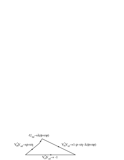
Figure 14: The $b-d$ unitarity quadrangle scaled by $A\lambda^{3}$, with sides given as above.

We see that unitarity requires that the length of the FCNC coupling side $-U^{*}_{db}$ has to be cancelled by another triangle side to close the triangle, and that occurs in $V^{*}_{tb}V_{td}$ having an addition to the SM formula. The area of the $b-d$ unitarity quadrangle is computed by adding the areas of three sub-triangles and a rectangle

$${\rm Area}(b-d)=A^{2}\lambda^{6}\left[\eta+(1-\rho)\psi\right]/2.$$ (65)

We note that if either or both $\eta$ and $\psi$ are non-zero, $CP$ is violated, and the quadrangle has a non-zero area, analogous to the SM unitarity triangle result. However, as we will see below, the area of the $b-d$ quadrangle is different from those of the other unitarity quadrangles by the $\psi$ term above.

VI.7.2 $s-b$ Quadrangle

The unitarity orthogonality between the $s$ and $b$ columns for the $s-b$ quadrangle is

$$V^{*}_{us}V_{ub}+V^{*}_{cs}V_{cb}+V^{*}_{ts}V_{tb}-U_{sb}=0.$$ (66)

The first term is $A\lambda^{4}(\rho-i\eta)$, the second term is $A\lambda^{2}$, and the third term is $-A\lambda^{2}$, to leading order. If we scale the base to unit length by dividing by $A\lambda^{2}$, then the first term side is of order 0.02 in length. From Fig. 15, the fourth side of scaled $U_{sb}$ is of order 0.0001, or 0.5% of the small third side of the triangle. The enclosed angle is then the same as in the SM, $\phi_{s}=\lambda^{2}\eta$, and the triangle’s or quadrangle’s area is $A^{2}\lambda^{6}\eta/2$.

Figure 15: Contours for the complex FCNC coupling $U_{sb}$ scaled by $|V^{*}_{cs}V_{cb}|$, which is the fourth side of the $s-b$ unitarity quadrangle.

VI.7.3 $d-s$ Quadrangle

Figure 16: Contours for the complex FCNC coupling $U_{ds}$ which is the fourth side of the $d-s$ unitarity quadrangle.

The orthogonality relation between the $d$ and $s$ columns is

$$V^{*}_{ud}V_{us}+V^{*}_{cd}V_{cs}+V^{*}_{td}V_{ts}-U_{ds}=0.$$ (67)

The largest sides of the $d-s$ unitarity quadrangle are of length $\lambda$, being the first and second terms, and the third term is $A^{2}\lambda^{5}(1-\rho+i\eta)=0.0004(1-\rho+i\eta)$. The fourth side is the FCNC coupling $U_{sd}$, which is bounded in magnitude by $2.5\times 10^{-5}=\lambda^{7}$, as seen in Fig. 16. Thus the FCNC fourth side is at most 6% of the small third side. The angle subtended by the small third side is then essentially the same as that by the third and fourth sides, being $\phi_{d}=A^{2}\lambda^{4}\eta$. The triangle’s or quadrangle’s area is also $A^{2}\lambda^{6}\eta/2$.

VI.8 The Sum Rule for the $CP$ violating $B$ Decay Asymmetry Angles

It was shown before Nir and Silverman (1990a) that as long as the Penguin diagrams in the $B$ decays can be neglected, that the sum of the $CP$ violating decay angles, even with new physics contributions, is $\pi$ modulo $\pi$. This can be seen from Eqs. (12) and (11) where in the sum of $(2\alpha+2\beta)$, the $B_{d}$ mixing phase cancels out in general, regardless of its source, and from Eqs. (13) and (16), where in the sum of $(2\gamma+4\phi_{s})$, the phase from $B_{s}$ mixing cancels out. The other tree amplitude decay phases in these equations either cancel or sum to the phase of a product of mixing matrix elements which becomes a product of absolute values squared, with zero phase. This leads to the $CP$ violating $B$ decay angle sum rule Nir and Silverman (1990a)

$$\alpha+\beta+\gamma+2\phi_{s}=\pi,\quad{\rm mod~{}}\pi.$$ (68)

VII Conclusions for Iso-singlet Down Quark Models

With much new data, it is still the case that FCNCs can contribute significantly to $B_{d}-\bar{B_{d}}$ mixing and to $B_{s}-\bar{B}_{s}$ mixing, and give contributions with new phases. In the FDQM, all $\sin{(2\alpha)}$ are allowed. In the $(\rho,\eta)$ plane, the FDQM allows large regions for $\rho\leq 0$ as opposed to the $\rho\geq 0$ regions in the SM, and in particular, those where $\eta$ goes to zero, both with the present data and with the projected $\sin{(2\alpha)}$ values. In new physics models then, the SM phase $\delta$, or $\eta$, can be smaller, with the other phases causing much of the presently observed $CP$ violation. In the $(x_{s},\sin{(\gamma)})$ plots in the FDQM, all of $\sin(\gamma)\geq 0$ is allowed at present in contrast to $\sin(\gamma)\geq 0.55$ in the SM, and with no approximately linear relation as in the SM. This will require combining experimental results of $x_{s}$ and $\sin{(\gamma)}$, to find out if the results correlate to the narrow linear region of the SM analysis. The present range for $x_{s}$ is from 16 to 48 at 2-$\sigma$ in the SM, and from 16 to 80 at 2-$\sigma$ in the four down quark model. The $b-d$ unitarity triangle, scaled to unit base length, has to be measured to an accuracy of 0.15 or better to begin to limit a fourth side and to verify the SM against the FDQM.

Each E₆ generation also contains an iso-singlet Hewett and Rizzo (1989) or sterile neutrino, which may provide a connection between the quark and lepton searches for new physics in terms of establishing new particle representations.

The mass of the lightest singlet down quark in E₆ could be roughly related to the mixing angle by

$$\theta_{34}^{2}\simeq m_{b}/m_{D},\quad{\rm and~{}with}~{}~{}|V_{4b}|\simeq\theta_{34}\leq 0.02$$ (69)

from combined fits, that gives

$$m_{D}\geq 2500\times m_{b}=11\ {\rm TeV}.$$ (70)

Using the single $R_{b}$ 90% CL limit of $|\theta_{34}|\leq 0.035$, which is not as strong as the combined fits, gives $m_{D}\geq 4$ TeV. The previous analysis Silverman (1998a) gave a lower limit of 1.2 TeV.