hep-ph/0205010

SHEP 02-06

Supersymmetric Higgs Bosons in a 5D Orbifold Model

V. Di Clemente, S. F. King and D. A. J. Rayner

Department of Physics and Astronomy, University of Southampton,
Southampton, SO17 1BJ, U.K.

1 Introduction

Extra-dimensional supersymmetric models with a TeV compactification scale [1] have recently offered an exciting new environment for investigating electroweak symmetry breaking (EWSB) [2, 3, 4, 5, 6]. The main features of these types of models are the following: (i) they provide a new mechanism to break supersymmetry (SUSY); (ii) the contribution of quark/squark Kaluza-Klein (KK) modes to the Higgs mass term is negative, thus triggering EWSB at the TeV scale; (iii) the 1-loop radiative correction to the effective potential is free of ultraviolet divergences, which implies that the Higgs physics is completely independent of the high-energy physics above some cutoff scale. Remarkably, the requirement of ${\mathcal{N}}=1$ SUSY in 5D (which is equivalent to ${\mathcal{N}}=2$ SUSY in 4D after compactification ) leads to a finite 1-loop effective potential because even though SUSY is globally softly broken, it is still preserved locally [4, 7] .

Various models have been proposed to study EWSB in extra dimensions and their phenomenological implications [2, 3, 4, 5, 6]. However we will concentrate only on those models which recover the MSSM below the compactification scale and are anomaly-free after the orbifold compactification [9]. The authors of Ref. [4] have made a qualitative study of the Higgs physics in their model, but there is little discussion of the phenomenological implications. In contrast, the authors of Ref. [5] have made an extensive study of Higgs phenomenology in their model and consider how radiative corrections modify the quadratic and quartic couplings of the tree-level potential. However, their approach neglects the non-renormalizable operators that arise at higher-order in the expansion of the full effective potential at 1-loop and, as discussed in the Appendices, this brings into question the reliability of their calculation.

In this paper we show that the conventional MSSM lightest Higgs boson mass bound $m_{h^{0}}\stackrel{{\scriptstyle<}}{{{}_{\sim}}}135$ GeV  [10] can be violated by allowing some of the fields to live in a fifth extra dimension . Motivated by fine-tuning arguments, we are led to an upper bound on the compactification scale $M_{C}\stackrel{{\scriptstyle<}}{{{}_{\sim}}}4$ TeV. At this compactification scale, the lightest Higgs boson mass can be pushed as high as $m_{h^{0}}\sim 160\,{\mathrm{G}eV}$. We find that in order to have EWSB through radiative corrections, $\tan\beta$ can have a wide range $1.5\stackrel{{\scriptstyle<}}{{{}_{\sim}}}\tan\beta\stackrel{{\scriptstyle<}}{{{}_{\sim}}}20$ rather than the small range allowed by Ref. [5] $35\stackrel{{\scriptstyle<}}{{{}_{\sim}}}\tan\beta\stackrel{{\scriptstyle<}}{{{}_{\sim}}}40$. We only limit $\tan\beta\stackrel{{\scriptstyle<}}{{{}_{\sim}}}20$ since we neglect bottom-sbottom loop effects. Note that, unlike the MSSM, $\tan\beta\approx 1.5$ is not ruled out by experiment in our extra dimensional model.

The layout of the remainder of the paper is as follows. In section 2 we review our 5D orbifold model, and in section 2.1 we discuss the top/stop sector KK mass spectra. In section 2.2 we discuss the Higgs SUSY breaking parameters. In section 2.3 we discuss how perturbativity and naturalness provide a constraint on the theory cutoff $M_{\ast}$. Then in section 3 we minimize the 1-loop effective potential and calculate the Higgs mass eigenvalues. We find that experimental data and fine-tuning arguments allow us to constrain the physical parameter space. Section 4 concludes the paper.

2 Our Model

In this section we review some basic features of our model [6] in which the extra dimension of a 5D theory is compactified on an $S^{1}/Z_{2}$ orbifold.

Figure 1: Our model showing the parallel 3-branes spatially separated along the extra dimension y. This extra dimension is compactified on the orbifold $S^{1}/Z_{2}$ that leads to two fixed points at $y=0,\pi R$, where the two 3-branes are located. The first two chiral families ($\hat{F}_{1,2}$) live on the Yukawa brane at $y=0$, while SUSY is broken by the F-term of a gauge singlet field ($\hat{S}$) on the source brane at $y=\pi R$. The third family ($\hat{F}_{3}$), gauge sector ($\hat{\mathcal{V}}_{MSSM}$) and Higgs superfields ($\hat{H}_{u,d}$) live in the extra dimensional bulk along with their ${\mathcal{N}}=2$ SUSY partners which are required for consistency.

The orbifold compactification leads to a description of 5D bulk fields as infinite towers of 4D KK-modes, and a classification of bulk fields into odd and even $Z_{2}$ parity . The $k^{th}$ KK-mode has a mass $m_{k}\sim{\mathcal{O}}\left(k\,M_{C}\right)$, where $M_{C}=1/R$ is the compactification scale, and the lowest KK resonance (k=0) can be identified with the usual MSSM fields. It is conventional in five-dimensional orbifold models to exploit the equivalence of ${\mathcal{N}}=1$ SUSY in 5D and ${\mathcal{N}}=2$ SUSY in 4D [13]. Therefore, an ${\mathcal{N}}=1$ multiplet in 5D can be decomposed into a 4D ${\mathcal{N}}=1$ chiral multiplet and its CP-conjugate “mirror” which together form a complete ${\mathcal{N}}=2$ hypermultiplet in 4D. Similarly, an ${\mathcal{N}}=1$ vector multiplet in 5D can be decomposed into a vector and chiral multiplet in 4D . The setup is given in Figure 1 and shows the location of the superfields within the extra-dimensional space.

We localized 4D 3-branes at the two fixed points $y=0,\pi R$ arising from the orbifold compactification. SUSY is broken on the “source” brane at $y=\pi R$ when a localized gauge field singlet ($\hat{S}$) acquires a non-zero F-term vacuum expectation value (VEV) $F_{S}$. The first two MSSM ($\hat{F}_{1,2}$) families are confined to the “Yukawa” brane  at $y=0$, while the third family ($\hat{F}_{3}$), MSSM gauge sector ($\hat{\mathcal{V}}_{MSSM}$) and Higgs superfields ($\hat{H}_{u,d}$) live in the extra dimensional bulk . These bulk fields acquire tree-level soft parameters due to their direct coupling with the SUSY breaking brane through non-renormalizable operators defined at $y=\pi R$:

$$\delta{\cal L}_{\pi R}=-\delta(y-\pi R)\int\!\!d^{4}\theta\left[\frac{1}{M_{\ast}^{3}}\left[c_{F_{3}}\hat{F}_{3}^{\dagger}\hat{F}_{3}+c_{H_{u}}\hat{H}_{u}^{\dagger}\hat{H}_{u}+c_{H_{d}}\hat{H}_{d}^{\dagger}\hat{H}_{d}+\left(c_{B\mu}\hat{H}_{u}\hat{H}_{d}+h.c.\right)\right]\hat{S}^{\dagger}\hat{S}\right.$$

$$+\left.\left(\frac{c_{\mu}}{M_{\ast}^{2}}\hat{H}_{u}\hat{H}_{d}\hat{S}^{\dagger}+h.c.\right)\right]\hskip 42.67912pt$$ (1)

where $M_{*}$ is the cutoff of the theory, and is often identified with the string scale. The coefficients $c_{F_{3}}(c_{H_{u,d}},c_{\mu},c_{B\mu})$ are the couplings of the third family (Higgs) superfields to the SUSY breaking sector. There are also higher-dimensional Yukawa couplings localized on the Yukawa brane at $y=0$, but we will only consider the dominant top/stop sector couplings:

$$\delta{\cal L}_{0}^{Yuk}=-\delta(y)\,\frac{f_{t}}{M_{\ast}^{3/2}}\int\!\!d^{2}\theta\left(\hat{Q}_{3L}\,\hat{H}_{u}\,\hat{U}_{3R}^{c}+h.c.\right)$$ (2)

where $f_{t}=(\pi RM_{\ast})^{3/2}\,y_{t}$ and $f_{t}(y_{t})$ is the 5d (4d) Yukawa coupling. The zero modes of the neutral components of the two complex (scalar) Higgs doublets can be expanded in terms of real and imaginary parts

$$H_{u}^{0}=\frac{1}{\sqrt{2}}\left(h_{u}+i\chi_{u}\right)\quad\quad H_{d}^{0}=\frac{1}{\sqrt{2}}\left(h_{d}+i\chi_{d}\right)$$ (3)

and electroweak symmetry is spontaneously broken when the real parts acquire non-zero VEVs $<h_{u}>,<h_{d}>\neq 0$ and $<\chi_{u}>=<\chi_{d}>=0$.

This setup is like the gaugino mediated SUSY breaking ($\tilde{g}$MSB) scenario [14], but with the third family superfields moved from the Yukawa brane and placed in the extra-dimensional bulk. The spatial separation of MSSM fields on the Yukawa brane away from the SUSY breaking sector alleviates the supersymmetric flavour-changing neutral-current (FCNC) problem since squark masses, arising from direct couplings between the two sectors, are exponentially suppressed by the separation between branes. Instead, first and second family squark masses are generated via flavour-blind loop-effects . Unlike previous models, our setup is motivated by a type I string-inspired model [16] in which the separation of the third family is generic, and often leads to realistic Yukawa textures.

2.1 Top/Stop KK Mass Spectra

We will summarize the KK mass spectra found in our earlier paper [6]. The non-renormalizable operators in Eq.(1) contain a delta-function that induces mixing between different KK-modes, where the mixing strengths ($\alpha_{\tilde{t}},\alpha_{H}$) are proportional to the SUSY breaking VEVs:

$$\alpha_{\tilde{t}}=c_{\tilde{t}}\pi\left(\frac{F_{S,\tilde{t}}^{2}}{M_{*}^{4}}\right)\left(\frac{M_{*}}{M_{C}}\right)\hskip 28.45274pt,\hskip 28.45274pt\alpha_{H}=c_{H}\pi\left(\frac{F_{S,H}^{2}}{M_{\ast}^{4}}\right)\left(\frac{M_{\ast}}{M_{C}}\right)$$ (4)

where $F_{S,\tilde{t}}(F_{S,H})$ is the F-term VEV associated with the singlet $\hat{S}$ field that couples to the stop (Higgs) fields . We have made the simplifying assumption that $c_{H_{u}}=c_{H_{d}}=c_{H}$. The non-trivial mixing between different KK-modes requires that we diagonalize an infinite mass matrix to obtain the KK mass eigenvalues . However, if the mixing is small, the mass matrix is dominated by the diagonal components. In order to respect ${\mathcal{N}}=1$ SUSY transformations on the brane, we use an off-shell formulation of ${\mathcal{N}}=2$ SUSY in the 5D bulk [13] that mixes fields of different $Z_{2}$-parity and so the KK-summation runs over the full tower ($-\infty<k<\infty$).

The field-dependent top KK-mode mass eigenvalues are given by :

$$m_{t,k}[h_{u}]=\left|kM_{C}+\frac{M_{C}}{\pi}\arctan\left(\frac{y_{t}\,h_{u}\,\pi}{\sqrt{2}M_{C}}\right)\right|\quad\quad(k=-\infty,\dots,\infty)$$ (5)

where the eigenvalues only depend on the real part of $H_{u}^{0}$. The observable top mass is identified with the $k=0$ KK-mode,

$$m_{t}[h_{u}]=\frac{M_{C}}{\pi}\arctan\left(\frac{y_{t}\,h_{u}\,\pi}{\sqrt{2}M_{C}}\right)$$ (6)

Notice that we can recover the usual MSSM relation $m_{t}[h_{u}]=y_{t}h_{u}/\sqrt{2}$ in the limit that ${\mbox{M}_{C}\rightarrow\infty}$. Eq.(6) is different due to the non-trivial mixing between KK-modes on the Yukawa brane.

The field-dependent stop KK mass eigenvalues $m_{\tilde{t},k}[h_{u}]$ are solutions of the following transcendental equation

$$\frac{\pi\,m_{\tilde{t},k}[h_{u}]}{M_{C}}\,\left[\tan\left(\frac{\pi\,m_{\tilde{t},k}[h_{u}]}{M_{C}}\right)-\left(\frac{\pi\,y_{t}\,h_{u}}{\sqrt{2}M_{C}}\right)^{2}\,\cot\left(\frac{\pi\,m_{\tilde{t},k}[h_{u}]}{M_{C}}\right)\right]=\alpha_{\tilde{t}}\left[1+\left(\frac{\pi\,y_{t}\,h_{u}}{\sqrt{2}M_{C}}\right)^{2}\right]$$ (7)

which can be solved by considering different limits of mixing $\alpha_{\tilde{t}}$.

Minimal mixing ($\alpha_{\tilde{t}}\ll 1$) is equivalent to a very small extra dimension ($M_{C}\sim 10^{16}$ GeV) where we expect to recover the MSSM results. The stop KK mass eigenvalues are :

$$m_{\tilde{t},k}^{2}[h_{u}]=\left[\left(k+\frac{m_{t}[h_{u}]}{M_{C}}\right)^{2}+\frac{\alpha_{\tilde{t}}}{\pi^{2}}+Z_{k}^{2}[h_{u},\alpha_{\tilde{t}}]\right]M_{C}^{2}\left[\vrule width=0.0pt,height=18.0pt1+{\cal O}(\alpha_{\tilde{t}}^{2})\right]\qquad(k=-\infty,\dots,\infty)$$ (8)

where we have used the field-dependent top mass $m_{t}[h_{u}]$ from Eq.(6), and the function $Z_{k}^{2}[h_{u},\alpha_{\tilde{t}}]$ is given by:

$$\begin{array}[]{rl}Z_{k\neq 0}^{2}[h_{u},\alpha_{\tilde{t}}]=&\left\{\begin{array}[]{lcl}\alpha_{\tilde{t}}/{\pi^{2}}&&\mbox{if}<h_{u}>=0\\ 0&&\mbox{otherwise}\end{array}\right.\\ Z_{k=0}^{2}[h_{u},\alpha_{\tilde{t}}]=&0\\ \end{array}$$ (9)

In the limit that electroweak symmetry remains unbroken (i.e. $<h_{u}>=0$), we find that only the even-parity bulk stop KK-modes acquire soft masses from the non-renormalizable operators of Eq.(1), while the odd parity stops have the usual KK masses ($m_{\tilde{t},k}^{odd}=kM_{C}$). Therefore the KK-summation only runs over the positive tower ($0<k<\infty$). Following EWSB ($<h_{u}>\neq 0$), the Yukawa interaction of Eq.(2) induces mixing between different parity stop KK-modes, and the KK-summation recovers the full infinite tower. Comparing Eqs.(5) and (8), we can see that the form of the $k=0$ mass eigenvalues resemble the MSSM as expected  where the stop mass squared is given by the top mass and SUSY breaking mass added in quadrature. However, in this limit the compactification scale $M_{C}$ can be at very high energies, and we recover the MSSM phenomenology at low energy.

Therefore, we consider maximal mixing in the stop sector ($\alpha_{\tilde{t}}\gg 1$) which is equivalent to a large extra dimension. In this case, the solution of Eq. (7) is given by

$$m_{\tilde{t},k}^{2}=\left(k+\frac{1}{2}\right)^{2}M_{C}^{2}\left[\vrule width=0.0pt,height=16.0pt1+{\cal O}\left(\alpha_{\tilde{t}}^{-1}\right)\right]\qquad\quad(k=-\infty,\dots,\infty)$$ (10)

Note that to leading order the stop mass eigenvalues are independent of the Higgs background field ($h_{u}$) even when the electroweak symmetry is broken. This can be attributed to the arbitrarily large mixing term on the source brane that makes the Yukawa brane become “transparent” which washes out any field dependence [6]. The Yukawa interaction induces mixing between different parity stop fields on the Yukawa brane such that both odd and even-parity stop KK-modes acquire the same mass from Eq.(10). We find that the compactification scale should be $M_{C}\approx{\mathcal{O}}({\mathrm{T}eV})$ to provide soft terms at the electroweak scale .

We use dimensional regularization and zeta-function regularization techniques [18] to evaluate the top/stop contributions to the 1-loop effective potential:

$$V_{1-loop}=V_{top}\,[h_{u}]+V_{stop} = \frac{1}{2}Tr\sum_{k=-\infty}^{\infty}\int\!\!\frac{d^{4}p}{\left(2\pi\right)^{4}}\ln\left[\frac{p^{2}+m_{\tilde{t},k}^{2}}{p^{2}+m_{t,k}^{2}\,[h_{u}]}\right]$$

$$= \frac{9M_{C}^{4}}{16\pi^{6}}\sum_{n=1}^{\infty}\frac{\cos\left[2\pi\,n\,m_{t}[h_{u}]/M_{C}\right]}{n^{5}}\,\,+\,\,\frac{135\,\zeta[5]}{256\pi^{6}}M_{C}^{4}\hskip 28.45274pt$$

where we have used Eqs.(5),(6) and (10), and the trace is over all degrees of freedom. The top and stop contributions are found to be separately finite (and free of ultraviolet divergences). However, we find the same result by using other regularization techniques (i.e. KK-regularization [2, 3, 4, 5]), where the UV divergences vanish due to supersymmetric cancellations between the top and stop contributions. Note that only the top contribution is field dependent, so the constant stop contribution can be absorbed into the cosmological constant and dropped from the subsequent analysis .

2.2 SUSY Breaking Higgs Parameters

We have seen in section 2.1 that we are led to maximal mixing ($\alpha_{\tilde{t}}\gg 1$) in the stop sector. We also know that for EWSB via top/stop radiative corrections, we require a negative mass-squared to trigger spontaneous symmetry breaking. This is harder to achieve when $\alpha_{\tilde{t}}\approx\alpha_{H}$ since this leads to tree-level and (negative) 1-loop contributions of comparable magnitude. Therefore, we conclude that the KK-modes in the Higgs sector must be minimally mixed (i.e. $\alpha_{H}\ll 1$).

Using Eq.(4), we have two options, either (i) the couplings in the higher-dimensional operators are hierarchical ($c_{\tilde{t}}\gg c_{H}$), or else (ii) there is a non-univerality in the hidden sector where different SUSY breaking fields couple to the stop and Higgs sectors ($F_{S,H}\neq F_{S,\tilde{t}}$). In this paper, we will assume that all hidden sector couplings are $c\sim{\mathcal{O}}(1)$, and instead have non-universal F-terms ($F_{S,H}\ll F_{S,\tilde{t}}$).

For minimal mixing in the Higgs sector, the KK mass matrix is dominated by the diagonal terms and we can decouple the non-zero KK excitations. We will impose the EWSB conditions on the lightest ($k=0$) KK-modes where the soft masses are taken directly from Eq.(1):

$$m_{H_{u}}^{2}=m_{H_{d}}^{2}=m_{soft}^{2}=\frac{c_{H}F_{S,H}^{2}}{M_{\ast}^{3}\,\pi}M_{C}\hskip 14.22636pt,\hskip 14.22636ptB\mu=\frac{c_{B\mu}F_{S,H}^{2}}{M_{\ast}^{3}\,\pi}M_{C}\hskip 14.22636pt,\hskip 14.22636pt\mu=\frac{c_{\mu}F_{S,H}}{M_{\ast}^{2}\,\pi}M_{C}$$ (12)

and we have assumed that $c_{H_{u}}=c_{H_{d}}=c_{H}$ for universal soft Higgs masses.

2.3 Reliability and Perturbativity

We have not yet imposed any constraint on the relationship between the compactification scale $M_{C}$ and the cutoff scale $M_{\ast}$. The requirement of perturbativity (where our perturbative analysis is valid) allows us to find an upper bound on the ratio $(M_{*}/M_{C})$. It is well known that in 5D (extra-dimensional) theories that the gauge and Yukawa couplings exhibit power law running behaviour [19]. The beta functions of these couplings depend on powers of the renormalization scale $\mu$ due to the inclusion of the KK-modes that makes the physics highly sensitive to the renormalization scale. This implies that gauge coupling unification and the emergence of the Landau pole in the Yukawa couplings are accelerated with respect to the (logarithmically-running) 4D theory. The top Yukawa coupling is found to become singular at energies close to the compactification scale $M_{C}$. In our model, the presence of the third family in the 5D bulk makes the Yukawa coupling beta function ($\beta_{y_{t}}$) depend quadratically on the ratio between the renormalization scale $\mu$ and the compactification scale $M_{C}$

$$\beta_{y_{t}}\sim y_{t}^{3}\left(\frac{\mu}{M_{C}}\right)^{2}+\ldots$$ (13)

Note that the dependence on $(\mu/M_{C})$ is stronger than the corresponding beta function for the gauge coupling ($\beta_{y_{t}}$) which is only linearly-dependent

$$\beta_{g}\sim g^{3}\left(\frac{\mu}{M_{C}}\right)+\ldots$$ (14)

Suppose $\mu_{NP}$ is the scale where the top Yukawa coupling becomes non-perturbative, which we numerically found to be $\mu_{NP}\approx 5M_{C}$  [5]. We can maintain a (reliable) perturbative regime by imposing the following constraint on the cutoff scale of our theory $M_{\ast}$

$$M_{\ast}\stackrel{{\scriptstyle<}}{{{}_{\sim}}}\mu_{NP}\hskip 28.45274pt\longrightarrow\hskip 28.45274ptM_{\ast}\stackrel{{\scriptstyle<}}{{{}_{\sim}}}5M_{C}$$ (15)

Similarly it appears “unnatural” to have the cutoff of our theory $M_{\ast}$ below the compactification scale $M_{C}$. Hence, we find that perturbativity and naturalness severely constrain $M_{\ast}$ to the range:

$$M_{C}\stackrel{{\scriptstyle<}}{{{}_{\sim}}}M_{\ast}\stackrel{{\scriptstyle<}}{{{}_{\sim}}}5M_{C}$$ (16)

We need to check that these constraints are consistent with maximal mixing in the stop sector ($\alpha_{\tilde{t}}\gg 1$). However, we find that there is no inconsistency since our earlier work [6] showed numerically that maximal mixing only requires $\alpha_{\tilde{t}}\stackrel{{\scriptstyle>}}{{{}_{\sim}}}12$ since solutions of Eq.(7) tend towards an asymptotic value with the stop mass eigenvalues given by Eq.(10). This is achieved when $F_{S,\tilde{t}}\stackrel{{\scriptstyle>}}{{{}_{\sim}}}(0.9/c_{\tilde{t}})M_{*}^{2}\approx M_{\ast}^{2}$ for $c_{\tilde{t}}\approx 1$.

3 Higgs Mass Spectrum

In this section we calculate the mass eigenvalues in the Higgs sector, where the light and heavy CP-even higgs mass eigenstates ($h^{0},H^{0}$) are linear combinations of the real fields $h_{u}$ and $h_{d}$. We can use the standard MSSM relations to find the masses of the charged ($H^{\pm}$) and CP-odd ($A^{0}$) Higgs fields. The tree-level potential in terms of the neutral components of the Higgs doublets ($H_{u}^{0},H_{d}^{0}$) is:

$$V_{tree}=m_{1}^{2}\left|H_{d}^{0}\right|^{2}+m_{2}^{2}\left|H_{u}^{0}\right|^{2}-B\mu\left(H_{u}^{0}H_{d}^{0}+h.c.\right)+\frac{m_{Z^{0}}^{2}}{2v^{2}}\left[\left|H_{u}^{0}\right|^{2}-\left|H_{d}^{0}\right|^{2}\right]^{2}$$ (17)

where we are free to define $B\mu$ as real and positive by absorbing any phase into $H_{u}^{0}$ and $H_{d}^{0}$; and we have traded the $U(1)_{Y}$ and $SU(2)_{L}$ gauge couplings ($g^{\prime},g$) for the physical $Z^{0}$ mass and the VEV $v=246$ GeV. The soft parameters $m_{1}^{2}=\left|\mu\right|^{2}+m_{H_{d}}^{2}$ , $m_{2}^{2}=\left|\mu\right|^{2}+m_{H_{u}}^{2}$ and $B\mu$ are given in Eq.(12).

Combining Eqs. (3,2.1,17), we find an expression for the total 1-loop effective potential in terms of the real Higgs fields $h_{u},h_{d}$. Notice that we have dropped the 1-loop stop contribution since it is independent of the Higgs fields and can be absorbed into the cosmological constant.

$$V=\frac{m_{soft}^{2}}{2}\left(h_{u}^{2}+h_{d}^{2}\right)-B\mu\,h_{u}h_{d}+\frac{m_{Z^{0}}^{2}}{8v^{2}}\left[h_{u}^{2}-h_{d}^{2}\right]^{2}+\frac{9M_{C}^{4}}{16\pi^{6}}\sum_{n=1}^{\infty}\frac{\cos\left[2n\tan^{-1}\left({\displaystyle\frac{y_{t}\,\pi\,h_{u}}{M_{C}\,\sqrt{2}}}\right)\right]}{n^{5}}$$ (18)

and we have assumed that the Higgs doublets acquire universal soft masses $m_{1}^{2}=m_{2}^{2}=m_{soft}^{2}$ which we regard as input parameters along with $B\mu$. Applying the EWSB conditions at the usual minimum $\left<h_{u}\right>=v\sin\beta\,,\,\left<h_{d}\right>=v\cos\beta$   ($v=246$ GeV)

$$\left.\frac{\partial V}{\partial h_{u}}\right|_{\left<h_{u}\right>,\left<h_{d}\right>}=\left.\frac{\partial V}{\partial h_{d}}\right|_{\left<h_{u}\right>,\left<h_{d}\right>}=0$$ (19)

allows us to eliminate $B\mu$ and $m_{Z^{0}}^{2}$ in terms of the other parameters. By imposing the correct observable $Z^{0}$ mass ($m_{Z^{0}}=91.2$ GeV), we can also eliminate $m_{soft}$ such that the compactification scale $M_{C}$ and $\tan\beta$ (or equivalently $m_{A^{0}}$) can be regarded as the two free parameters. In Figure 2, we plot $m_{soft}$ as a function of the compactification scale $M_{C}$ for two different values of $\tan\beta$.

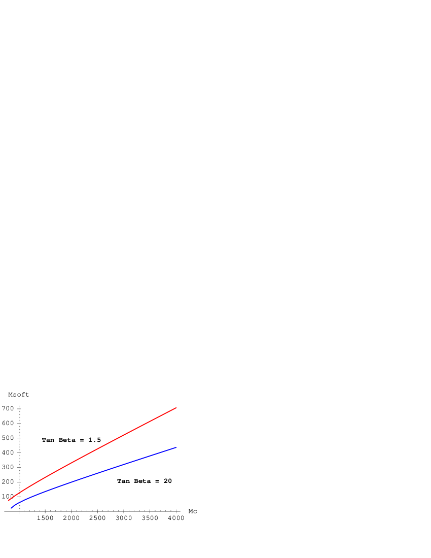
Figure 2: The universal Higgs soft mass $m_{soft}^{2}=\left|\mu\right|^{2}+m_{H_{u,d}}^{2}$ against the compactification scale $M_{C}$ for $\tan\beta=1.5$ and $20$.

We construct the CP-even mass matrix from the second derivatives of the effective potential at the minimum, which can be diagonalized to find the mass eigenvalues ($m_{h^{0}},m_{H^{0}}$):

$${\mathcal{M}}^{2}_{even}=\left(\begin{array}[]{cc}{\displaystyle\frac{\partial^{2}V}{\partial h_{u}^{2}}}&{\displaystyle\frac{\partial^{2}V}{\partial h_{u}\partial h_{d}}}\\ {\displaystyle\frac{\partial^{2}V}{\partial h_{d}\partial h_{u}}}&{\displaystyle\frac{\partial^{2}V}{\partial h_{d}^{2}}}\end{array}\right)$$ (22)

Notice that these CP-even eigenvalues include the 1-loop effects, but only $m_{2}^{2}$ is 1-loop improved since we are neglecting bottom-sbottom loops for $\tan\beta\leq 20$:

$$m_{2,imp}^{2}=m_{2}^{2}+\frac{1}{2}\left.\frac{\partial^{2}V_{top}}{\partial h_{u}^{2}}\right|_{\left<h_{u}\right>,\left<h_{d}\right>}$$ (23)

However $B\mu$ (and $m_{1}^{2}$) are not 1-loop improved, so we can use the standard 4D tree-level MSSM expressions to find the CP-odd ($A^{0}$) and charged Higgs ($H^{\pm}$) masses.

$$m_{A^{0}}^{2} = \frac{2B\mu}{\sin 2\beta}$$ (24)

$$m_{H^{\pm}}^{2} = m_{A^{0}}^{2}+m_{W}^{2}$$ (25)

We can solve for $m_{Z^{0}}^{2}$ as a function of the free parameters ($M_{C},\tan\beta$), and use the standard definition of fine-tuning $\Delta$  [20, 21] (but neglecting the variation of $\tan\beta$ with respect to changes in $M_{C}$) to find an upper limit on the compactification scale $M_{C}$.

$$\Delta=\left|\frac{M_{C}}{m_{Z^{0}}^{2}}\,\frac{\partial m_{Z^{0}}^{2}}{\partial M_{C}}\right|$$ (26)

Figure 3: The fine-tuning parameter $\Delta$ as a function of $\tan\beta$ and the compactification scale $M_{C}$ in GeV. $\Delta$ is shown to have a very weak dependence on $\tan\beta$ in the range $2.5\stackrel{{\scriptstyle<}}{{{}_{\sim}}}\tan\beta\stackrel{{\scriptstyle<}}{{{}_{\sim}}}20$ for which we can neglect bottom-sbottom effects. However, the fine-tuning becomes singular as $\tan\beta\rightarrow 1$.

Motivated by the fine-tuning as shown in Figure 3, we will investigate the parameter space $M_{C}\leq 4$ TeV and $1.5\leq\tan\beta\leq 20$ where the fine-tuning $\Delta\sim{\mathcal{O}}(10^{2})$.

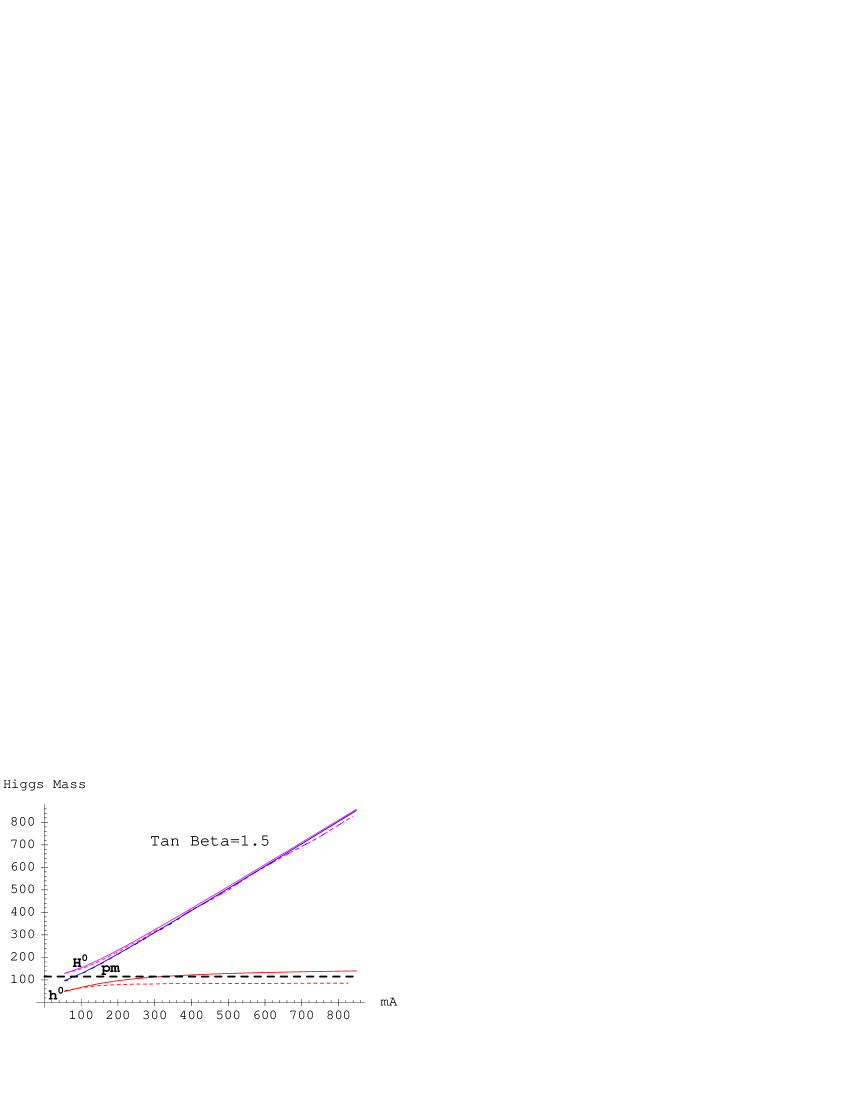
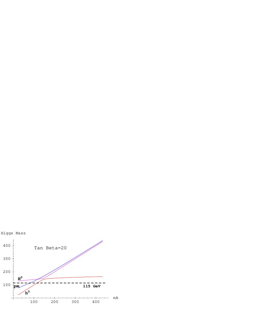
Figure 4: The Higgs masses ($m_{h^{0}},m_{H^{\pm}},m_{H^{0}}$) against $m_{A^{0}}$ for $\tan\beta=1.5$ (upper panel) and $\tan\beta=20$ (lower panel). We have run $1\leq M_{C}\leq 4$ TeV parametrically along each curve. The LEP candidate at 115 GeV (bold dotted-line)  [23] is shown for comparison with $m_{h^{0}}$. For $\tan\beta=1.5$ (upper panel), we also compare the MSSM results taken from [22] (dotted-lines) against our model (bold-lines).

In Figure 4, we plot the eigenvalues ($m_{h^{0}},m_{H^{0}}$) of the CP-even mass matrix and the charged Higgs mass ($m_{H^{\pm}}$) against the CP-odd mass ($m_{A^{0}}$) for two fixed values of $\tan\beta=1.5$ and $20$. We run the value of the compactification scale parametrically along each curve, $1\leq M_{C}\leq 4$ TeV. We also include the MSSM predictions for $\tan\beta=1.5$ taken from [22] for comparison. Notice that unlike the MSSM predictions from [22], our model is not excluded by the LEP signal for $\tan\beta=1.5$. There are additional experimental lower limits for the other Higgs masses

$$m_{A^{0}}\geq 92\,{\mathrm{G}eV\hskip 28.45274ptand}\hskip 28.45274ptm_{H^{\pm}}\geq 69\,{\mathrm{G}eV}$$ (27)

but these provide a much weaker constraint on our model.

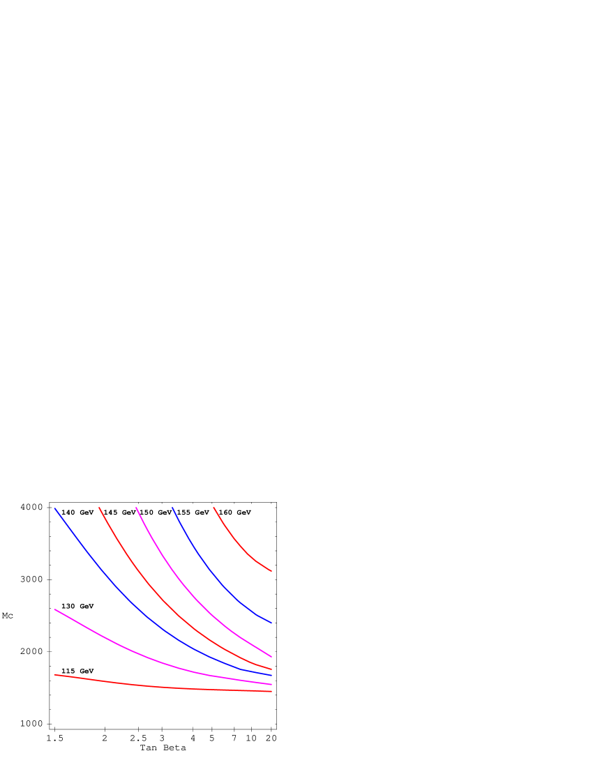
Figure 5: Mass contour plot for the lightest Higgs mass $m_{h^{0}}$ as a function of the compactification scale $M_{C}$ (GeV) and $\tan\beta$ in the absence of bottom sector effects (i.e. $\tan\beta\leq 20$). The LEP candidate at 115 GeV  [23] is easily accommodated over the range of $\tan\beta$ with a compactification scale $M_{C}\approx 1.5-1.7$ TeV. At large $\tan\beta\rightarrow 20$ and $M_{C}\rightarrow 4$ TeV, the lightest Higgs mass can be as large as $m_{h^{0}}\sim 164$ GeV.

In Figure 5, we plot the lightest Higgs mass ($m_{h^{0}}$) as a function of the compactification scale $M_{C}$ and $\tan\beta$. The LEP data excludes the parameter space below the first contour at $m_{h^{0}}=115$ GeV  [23] which corresponds to a compactification scale $M_{C}\approx 1.5-1.7$ TeV over the whole range of $\tan\beta$. Combining Figures 3 and 5 we find an allowed window for the compactification scale

$$1.5\,{\mathrm{T}eV}\stackrel{{\scriptstyle<}}{{{}_{\sim}}}M_{C}\stackrel{{\scriptstyle<}}{{{}_{\sim}}}4\,{\mathrm{T}eV}$$ (28)

Notice that our model can easily accommodate the conventional 4D MSSM upper bound on the lightest Higgs boson mass $m_{h^{0}}\sim 130$ GeV, and can be pushed as high as $m_{h^{0}}\sim 160$ GeV with $M_{C}\approx 4$ TeV and $5\stackrel{{\scriptstyle<}}{{{}_{\sim}}}\tan\beta\stackrel{{\scriptstyle<}}{{{}_{\sim}}}20$. Remember that including additional matter (e.g. gauge singlets in the NMSSM) can also raise the upper bound on the lightest Higgs mass, but our “minimal” extension of the MSSM achieves higher mass bounds without adding extra matter content.

We can use Figure 2 to find limits on the $\mu$-parameter from the universal soft Higgs mass $m_{soft}$ which is constrained when we impose EWSB at the electroweak minimum. Using Eq.(12), we find the ratio between $m_{H_{u}}^{2}=m_{H_{d}}^{2}=m_{H}^{2}$ and $\left|\mu\right|^{2}$ in terms of the compactification and cutoff scales:

$$\frac{m_{H}^{2}}{\left|\mu\right|^{2}}\sim\frac{M_{\ast}\pi}{M_{C}}$$ (29)

where we have assumed that $c_{H},c_{\mu}\sim 1$.

Recall from section 2.2 that we assume non-universality in the SUSY breaking sector ($F_{S,H}\ll F_{S,\tilde{t}}$) to obtain maximal (minimal) mixing in the stop (Higgs) sectors for viable radiative EWSB without hierarchical couplings $c_{\tilde{t}}\sim c_{H}$. We can use the perturbativity and naturalness constraints of Eq.(16) to find limits on the ratio between the soft Higgs mass and the $\mu$-parameter from Eq.(29)

$$\pi\stackrel{{\scriptstyle<}}{{{}_{\sim}}}\frac{m_{H}^{2}}{\left|\mu\right|^{2}}\stackrel{{\scriptstyle<}}{{{}_{\sim}}}5\pi$$ (30)

and therefore limits on $m_{soft}$ in terms of $\mu$:

$$m_{soft}^{2}=m_{H}^{2}+\left|\mu\right|^{2}\hskip 28.45274pt\longrightarrow\hskip 28.45274pt(\pi+1)\,\left|\mu\right|^{2}\stackrel{{\scriptstyle<}}{{{}_{\sim}}}m_{soft}^{2}\stackrel{{\scriptstyle<}}{{{}_{\sim}}}(5\pi+1)\,\left|\mu\right|^{2}$$ (31)

The constraints on the $\mu$-parameter for different compactification scales and values of $\tan\beta$ are shown in Table 1:

	$M_{C}=1.5\,{\mathrm{T}eV}$	$M_{C}=4\,{\mathrm{T}eV}$
$\tan\beta=1.5$	$114\stackrel{{\scriptstyle>}}{{{}_{\sim}}}\left|\mu\right|\stackrel{{\scriptstyle>}}{{{}_{\sim}}}57$	$347\stackrel{{\scriptstyle>}}{{{}_{\sim}}}\left|\mu\right|\stackrel{{\scriptstyle>}}{{{}_{\sim}}}173$
$\tan\beta=20$	$66\stackrel{{\scriptstyle>}}{{{}_{\sim}}}\left|\mu\right|\stackrel{{\scriptstyle>}}{{{}_{\sim}}}33$	$215\stackrel{{\scriptstyle>}}{{{}_{\sim}}}\left|\mu\right|\stackrel{{\scriptstyle>}}{{{}_{\sim}}}107$

Table 1: Upper and lower limits on the size of the $\mu$-parameter for two different values of $\tan\beta=1.5$ and 20, and compactification scales $M_{C}=1.5$ and 4 TeV.

Therefore, the magnitude of the $\mu$-parameter is constrained to the range $33\stackrel{{\scriptstyle<}}{{{}_{\sim}}}\left|\mu\right|\stackrel{{\scriptstyle<}}{{{}_{\sim}}}347$ GeV.

4 Conclusions and Discussion

In conclusion we have considered the Higgs sector of an ${\mathcal{N}}=1$ supersymmetric 5D theory compactified on an orbifold $S^{1}/Z_{2}$ where the compactification scale $M_{C}\sim{\mathcal{O}}\left(TeV\right)$. Orbifolding leads to fixed points at either end of the extra dimension (y) where 4D branes can be localized. Supersymmetry is broken by the F-term VEV of a gauge singlet on the brane at $y=\pi R$ that is spatially separated from another Yukawa brane at $y=0$ where the first two MSSM families and Yukawa couplings are localized. Direct coupling between the two sectors (and therefore soft squark masses) are suppressed by the separation between the branes which alleviates the flavour-changing neutral-current problem since the first and second family squark masses are only generated through flavour-blind loops. The third family, gauge sector and Higgs fields live in the extra dimensional bulk with their ${\mathcal{N}}=2$ supersymmetric partners (which are required for consistency) and therefore receive unsuppressed soft masses due to their direct coupling to the SUSY breaking sector.

We assume a non-universality in the SUSY breaking sector, where different gauge singlets couple separately to the stop (Higgs) fields and the associated F-term VEVs are hierarchical ($F_{S,H}\ll F_{S,\tilde{t}}$) which induces maximal (minimal) mixing between different KK-modes. The maximal mixing between stop modes requires that we use a matrix method to diagonalize the infinite mass matrix. In contrast the Higgs KK-modes are minimally mixed so that the mass matrix is dominated by the diagonal components and we can decouple the non-zero KK-modes from the analysis. We find that the soft Higgs parameters are generated by non-renormalizable operators. The presence of the third family in the bulk is particularly important for their dominant 1-loop contribution to the Higgs effective potential. The full tower of top and stop Kaluza-Klein modes contribute to the potential and trigger radiative electroweak symmetry breaking. Following dimensional regularization and zeta-function regularization techniques, we see that the 1-loop contributions to the effective potential are separately finite and therefore insensitive to the high-energy cutoff $M_{\ast}$. However in the maximal mixing limit we find that the top contribution has a non-trivial dependence on the Higgs background fields, and the stop only contributes to the cosmological constant.

We minimize the 1-loop effective potential and impose the conditions for electroweak symmetry breaking to find the physical Higgs mass eigenvalues. Requiring the correct physical $Z^{0}$-mass allows us to eliminate parameters in terms of the compactification scale $M_{C}$ and $\tan\beta$ (or equivalently $m_{A^{0}}$). We use fine-tuning arguments to constrain our parameter space $M_{C}\stackrel{{\scriptstyle<}}{{{}_{\sim}}}4$ TeV, and we choose to study the region $1.5\stackrel{{\scriptstyle<}}{{{}_{\sim}}}\tan\beta\stackrel{{\scriptstyle<}}{{{}_{\sim}}}20$ where bottom sector effects can be neglected. We obtain physical Higgs mass eigenvalues for different values of $\tan\beta$ and find that the LEP signal [23] imposes a lower limit on the compactification scale $M_{C}\stackrel{{\scriptstyle>}}{{{}_{\sim}}}1.5$ TeV. We also find that, unlike the MSSM, $\tan\beta=1.5$ is not excluded by experiment and our model can accommodate the LEP signal over the full parameter space. In fact the usual MSSM upper bound ($m_{h^{0}}\stackrel{{\scriptstyle<}}{{{}_{\sim}}}130$ GeV) and the extended NMSSM bound ($m_{h^{0}}\stackrel{{\scriptstyle<}}{{{}_{\sim}}}150$ GeV) can be trivially exceeded and raised to $m_{h^{0}}\stackrel{{\scriptstyle<}}{{{}_{\sim}}}164$ GeV for a compactification scale $M_{C}\sim 4$ TeV and $5\stackrel{{\scriptstyle<}}{{{}_{\sim}}}\tan\beta\stackrel{{\scriptstyle<}}{{{}_{\sim}}}20$.

Note that radiative electroweak symmetry breaking is viable over a large range $1.5\stackrel{{\scriptstyle<}}{{{}_{\sim}}}\tan\beta\stackrel{{\scriptstyle<}}{{{}_{\sim}}}20$ in comparison to an alternative model  [5] that is severely constrained to the smaller range $35\stackrel{{\scriptstyle<}}{{{}_{\sim}}}\tan\beta\stackrel{{\scriptstyle<}}{{{}_{\sim}}}40$. In fact, we show in Appendix B that their diagrammatic analysis is incomplete because it neglects higher-order non-renormalizable operators that inevitably appear in the expansion of the 1-loop effective potential. The requirement of perturbativity and naturalness in our model imposes a constraint on the relationship between the compactification scale $M_{C}$ and the cutoff $M_{\ast}$ scale ($M_{C}\stackrel{{\scriptstyle<}}{{{}_{\sim}}}M_{\ast}\stackrel{{\scriptstyle<}}{{{}_{\sim}}}5M_{C}$). We use this constraint in combination with the universal soft Higgs mass to deduce limits on the $\mu$-parameter, and we find that the magnitude of $\mu$ is inside the range $33\stackrel{{\scriptstyle<}}{{{}_{\sim}}}\left|\mu\right|\stackrel{{\scriptstyle<}}{{{}_{\sim}}}347$ GeV.

Scherk-Schwarz (SS) boundary conditions have been used extensively in the literature to break SUSY in extra dimensional models [2, 3, 4, 5, 7]. Recently, the authors of Ref. [24] demonstrated that the SS effects are always present, and a vanishing SS parameter at tree-level will be generated at 1-loop by bulk supergravity fields . In the case that SUSY breaking is localized on a hidden sector brane, the SS breaking parameter $\omega_{SS}$ is no longer discrete, but may take a range of values that depend upon the relative strength of the SUSY breaking and the matter content of fields living in the extra dimension . In our model, the third family and Higgs hypermultiplets ($N_{H}=19$) live in the bulk with the MSSM vector multiplets ($N_{V}=12$), and the SS breaking parameter tends towards $\omega_{SS}=0$ ($\omega_{SS}=1/2$) for weak (strong) SUSY breaking on the brane which is equivalent to minimal (maximal) mixing in the stop sector.

We anticipate that non-trivial SS contributions will modify our expressions for the stop KK-mode mass eigenvalues  given in Eqs.(8,10). However, we can see that the additional SS contributions will not alter our analysis of the Higgs sector. For minimal mixing the stop mass eigenvalues are given by Eq.(8), but we know that in this limit the SS parameter vanishes. Also, for maximal mixing $\omega_{SS}\rightarrow 1/2$ and Eq.(10) becomes $m_{\tilde{t},k}^{2}=\left(k+1/2+\omega_{SS}\right)^{2}M_{C}^{2}+\ldots$. However, we have already seen that the stop mass eigenvalues are independent of the background Higgs field in this maximal mixing limit and the stop sector contribution to the effective potential is constant. Therefore, we find that Scherk-Schwarz effects play no rôle in our calculations and we are justified in ignoring them.

Acknowledgements

S.K., V.D.C. and D.R. would like to thank PPARC for a Senior Fellowship, Research Associateship and a Studentship. We would like to thank Antonio Riotto for useful discussions and bringing Ref. [24] to our attention.

Appendix A Finite Higgs Mass from a Diagrammatic Approach

In section 2.1 we have shown that in the limit the brane-localized SUSY breaking term associated with the stop sector is arbitrarily large (maximal mixing), the 1-loop effective potential only receives field-dependence from the top sector KK masses while the stop sector contribution can be absorbed into the cosmological constant. In this appendix we will show that the finite part of the 1-loop Higgs scalar two-point function at zero external momenta, as shown in Figure 6, only arises from the top KK-mode contributions. We illustrate this with a toy model that we have already discussed in earlier work [6].

Figure 6: One-loop diagrams contributing to $\delta m_{h}^{2}$ in Eq.(34). Notice that the second and third diagrams (b,c) appear in the MSSM while the requirement for ${\mathcal{N}}=2$ SUSY in the extra dimensional bulk leads to an additional diagram (a) involving CP-mirror partners.

In Ref. [6] we made the simplifying assumption that the tree level potential only receives D-term contributions by ignoring the Higgs soft parameters that are generated by non-renormalizable operators in Eq.(1). We made a further simplification by taking the limit $\tan\beta\rightarrow\infty$ where the $H_{d}$ doublet can be decoupled. Therefore, the tree-level potential is only a function of the neutral component of the up-type Higgs $H_{u}^{0}$ which we take to be real $h_{u}$ from Eq.(3)

$$V_{tree}[h_{u}]=\frac{g^{2}+g^{\prime 2}}{32}h_{u}^{4}$$ (32)

where $g$ and $g^{\prime}$ are the gauge couplings of $SU(2)_{L}$ and $U(1)_{Y}$ respectively. We can see that at tree-level the potential has a minimum at $h_{u}=0$. However, the 1-loop contributions can trigger electroweak symmetry to be spontaneously broken. The 1-loop contribution is given in Eq.(2.1). The full effective potential is then

$$V[h_{u}]=V_{tree}[h_{u}]+V_{1-loop}[h_{u}]$$ (33)

We find that a negative quadratic mass term is given by:

$$\delta m_{h}^{2}=\left.\frac{d^{2}V}{dh_{u}^{2}}\right|_{<h_{u}>=0}=-\frac{9\,\zeta(3)}{8\pi^{4}}\,y_{t}^{2}M_{C}^{2}\approx-\left(1.39\times 10^{-2}\right)\,y_{t}^{2}M_{C}^{2}$$ (34)

where $\zeta(3)\approx 1.202$. Notice that Eq.(34) is identical to the result reported in Ref. [4], where $\delta m_{h}^{2}$ was calculated using the diagrams shown in Figure 6. The mass eigenvalues of the even-parity stop KK-modes ($\tilde{t}_{R,l}$ and $\tilde{t}_{L,l}$) are given in Eq. (10); and the masses for the odd-parity (mirror) stops ($\tilde{t}_{R,k}^{mc}$ and $\tilde{t}_{L,k}^{mc}$) and the tops ($t_{L,k},t_{R,k}$) are $\sim kM_{C}$.

It is possible to see that the finite part of $\delta m_{h}^{2}$ effectively arises from diagram (b) in Figure 6 where only the top KK-modes propagate in the loop. Evaluating diagrams (a)+(c) gives:

$$-i\delta m_{h}^{2}\left[\vrule width=0.0pt,height=16.0pt\mbox{(a)+(c)}\right] = 3y_{t}^{2}\sum_{k=0}^{\infty}\sum_{l=0}^{\infty}\left(\eta_{k}\right)^{2}\int\!\!\frac{d^{4}p}{(2\pi)^{4}}\frac{m^{2}_{\tilde{t}_{L,k}^{mc}}}{(p^{2}-m^{2}_{\tilde{t}_{L,k}^{mc}})(p^{2}-m^{2}_{\tilde{t}_{R,l}})}+(L\leftrightarrow R)$$ (35)

$$+ 3y_{t}^{2}\sum_{k=0}^{\infty}\sum_{l=0}^{\infty}\left(\eta_{k}\right)^{2}\int\!\!\frac{d^{4}p}{(2\pi)^{4}}\frac{1}{(p^{2}-m^{2}_{\tilde{t}_{R,l}})}+(L\leftrightarrow R)$$

where the factor of $3$ is the colour multiplicity and $\eta_{k}=(1/\sqrt{2})^{\delta_{k0}}$. Numerous papers in the literature [18, 25] have demonstrated the validity of exchanging the sum and integral in Eq.(35) despite the controversy surrounding this so-called “KK-regularization” technique [26]. Performing a Wick rotation to Euclidean momentum space $p_{E}$, and a change of variables $x=p_{E}/M_{C}$ gives

$$-i\delta m_{h}^{2}\left[\vrule width=0.0pt,height=16.0pt\mbox{(a)+(c)}\right] = -i3y_{t}^{2}M_{C}^{2}\int\!\!\frac{d^{4}x}{(2\pi)^{4}}\,\sum_{k,l=0}^{\infty}\frac{(\eta_{k})^{2}x^{2}}{(x^{2}+(k+1/2)^{2})(x^{2}+l^{2})}$$ (36)

$$= -i3y_{t}^{2}M_{C}^{2}\frac{\pi^{2}}{4}\int\!\!\frac{d^{4}x}{(2\pi)^{4}}=-\frac{3\,i\,y_{t}^{2}}{128}\frac{\Lambda^{4}}{M_{C}^{2}}$$

where $\Lambda$ is the UV cutoff. The quartically-divergent contribution in Eq.(36) exactly cancels with the infinite part of diagram (b). Therefore, $\delta m_{h}^{2}$ in Eq.(34) only arises from diagram (b) .

We will conclude this appendix by calculating the compactification scale and Higgs mass in this toy model. We use the $\overline{{\mbox{M}S}}$ running top mass $m_{t,0}=166$ GeV to find the compactification scale by imposing the following minimization conditions around the minimum at $v=246$ GeV:

$$\left.\frac{dV}{dh_{u}}\right|_{<h_{u}>=v}=0\hskip 56.9055pt\left.\frac{d^{2}V}{dh_{u}^{2}}\right|_{<h_{u}>=v}=m_{h}^{2}$$ (37)

Numerically we find:

$$M_{C}\approx 830\,\,{\mathrm{G}eV}$$ (38)

which is approximately $2.5$ times larger than the compactification scale calculated in Ref. [3]. The second-derivative of the effective potential at the minimum yields a lightest Higgs scalar mass 

$$m_{h}\approx 120\,\,{\mathrm{G}eV}$$ (39)

This prediction for the lightest Higgs boson mass is possible because the effective potential just depends on the compactification scale $M_{C}$ which has been fixed at a specific value $M_{C}\approx 830$ GeV to obtain the correct minimum of the effective potential. However, the more general two-Higgs doublet analysis in section 3 depends on other soft parameters including $\tan\beta$, the universal soft Higgs mass $m_{soft}^{2}\,,\,B\mu$ and the supersymmetric mass $\mu$.

Appendix B Truncation of the 1-loop Effective Potential

In this appendix we discuss the problems that arise when truncating the expression of the full 1-loop effective potential in the context of extra dimensions. We will show that this truncation leads to a significant discrepancy compared to using the full 1-loop expression. This problem arises because all dimensionful parameters defined in the theory are of the same order $\sim M_{C}$. In the effective field theory, it is impossible to distinguish between high and low energy scales, and all non-renormalizable operators are found to be as important as the renormalizable operators.

Expanding the 1-loop effective potential (2.1) around the origin $h_{u}=0$ we obtain:

$$\tilde{V}_{1-loop}[h_{u}]=\frac{9\,\zeta(5)}{16\pi^{6}}M_{C}^{4}+\frac{1}{2}\delta m_{h}^{2}\,h_{u}^{2}+\frac{3\,y_{t}^{4}}{16\pi^{2}}h_{u}^{4}\left[\zeta(3)+\frac{25}{24}-\frac{1}{2}\log\left(\frac{\sqrt{2}\pi y_{t}\,h_{u}}{M_{C}}\right)\right]+{\cal O}\left(\frac{h_{u}^{6}}{M_{C}^{2}}\right)$$ (40)

where we have used the expression for $\delta m_{h}^{2}$ from Eq.(34) and tildes denote truncated results. Notice that all non-renormalizable operators ${\cal O}\left(h_{u}^{6}/M_{C}^{2}\right)$ vanish in the limit $M_{C}\rightarrow\infty$.

However, for $M_{C}\approx{\mathcal{O}}({\mathrm{T}eV})$, these higher-order operators will give an important contribution to the effective potential. Therefore, if the expansion is truncated at ${\mathcal{O}}(h_{u}^{4})$ we can no longer regard the results as reliable. For example, if we impose the minimization conditions of Eq.(37) on the truncated potential from Eq.(40) we find:

$$\tilde{M}_{C}\approx 1\,\,\mbox{TeV}\qquad\quad\tilde{m}_{h}\approx 170\,\,\mbox{GeV}$$ (41)

Comparing with the exact results from Eqs.(38,39), we see that the truncated approximation from Eq.(40) leads to an error of $(20-40)\%$.

We can easily understand the origin of this discrepancy by noting that the only dimensionful parameter that appears in the effective potential is the compactification scale $M_{C}$. Therefore, each operator in the expansion of Eq.(40) gives comparable contributions. Notice that the truncation of the series is equivalent to integrating out the top KK-tower. From the effective field theory perspective, this truncation must be controlled by an expansion in $\gamma=(m^{2}/M^{2})$, where $m$ is the low energy scale (for example the electroweak scale $M_{W}$) and $M$ is the high energy scale associated with the masses of the heavy particles $\sim M_{C}$.

In the case that $\gamma\ll 1$, the truncation of the series is reliable. However, in this model $m$ is generated at 1-loop and is proportional to $M=M_{C}$, where $m^{2}=\delta m_{h}^{2}$ from Eq.(34) but without the loop factor . Therefore $m^{2}\approx M^{2}\rightarrow\gamma\approx 1$, and we conclude that truncation of the effective potential expansion at finite order cannot be reliable. The same conclusion was observed in Ref. [3].

References

- [1] I. Antoniadis, Phys. Lett. B 246 (1990) 377.
- [2] A. Pomarol and M. Quiros, Phys. Lett. B 438 (1998) 255 [arXiv:hep-ph/9806263]; I. Antoniadis, S. Dimopoulos, A. Pomarol and M. Quiros, Nucl. Phys. B 544, 503 (1999) [arXiv:hep-ph/9810410]; A. Delgado, A. Pomarol and M. Quiros, Phys. Rev. D 60 (1999) 095008 [arXiv:hep-ph/9812489].
- [3] R. Barbieri, L. J. Hall and Y. Nomura, Phys. Rev. D 63 (2001) 105007 [arXiv:hep-ph/0011311].
- [4] N. Arkani-Hamed, L. J. Hall, Y. Nomura, D. R. Smith and N. Weiner, Nucl. Phys. B 605 (2001) 81 [arXiv:hep-ph/0102090].
- [5] A. Delgado and M. Quiros, Nucl. Phys. B 607 (2001) 99 [arXiv:hep-ph/0103058].
- [6] V. Di Clemente, S. F. King and D. A. J. Rayner, Nucl. Phys. B 617 (2001) 71 [arXiv:hep-ph/0107290].
- [7] A. Masiero, C. A. Scrucca, M. Serone and L. Silvestrini, Phys. Rev. Lett. 87, 251601 (2001) [arXiv:hep-ph/0107201].
- [8] A. Delgado, G. V. Gersdorff and M. Quiros, Nucl. Phys. B 613 (2001) 49 [arXiv:hep-ph/0107233].
- [9] D. M. Ghilencea, S. Groot Nibbelink and H. P. Nilles, Nucl. Phys. B 619 (2001) 385 [arXiv:hep-th/0108184]; C. A. Scrucca, M. Serone, L. Silvestrini and F. Zwirner, Phys. Lett. B 525, 169 (2002) [arXiv:hep-th/0110073]; L. Pilo and A. Riotto, arXiv:hep-th/0202144.
- [10] For a recent calculation of the 2-loop correction to the CP-even higgs mass in the MSSM, see for example J. R. Espinosa and I. Navarro, Nucl. Phys. B 615 (2001) 82 [arXiv:hep-ph/0104047]; G. Degrassi, P. Slavich and F. Zwirner, Nucl. Phys. B 611, 403 (2001) [arXiv:hep-ph/0105096]; A. Brignole, G. Degrassi, P. Slavich and F. Zwirner, arXiv:hep-ph/0112177, and references therein.
- [11] J. A. Casas, J. R. Espinosa and I. Navarro, Nucl. Phys. B 620 (2002) 195 [arXiv:hep-ph/0109127].
- [12] A. Falkowski, C. Grojean and S. Pokorski, arXiv:hep-ph/0203033.
- [13] E. A. Mirabelli and M. E. Peskin, Phys. Rev. D 58 (1998) 065002 [arXiv:hep-th/9712214].
- [14] D. E. Kaplan, G. D. Kribs and M. Schmaltz, Phys. Rev. D 62 (2000) 035010 [arXiv:hep-ph/9911293]; Z. Chacko, M. A. Luty, A. E. Nelson and E. Ponton, JHEP 0001 (2000) 003 [arXiv:hep-ph/9911323].
- [15] F. Gabbiani, E. Gabrielli, A. Masiero and L. Silvestrini, Nucl. Phys. B 477 (1996) 321 [arXiv:hep-ph/9604387].
- [16] S. F. King and D. A. J. Rayner, Nucl. Phys. B 607 (2001) 77 [arXiv:hep-ph/0012076].
- [17] R. Barbieri, L. J. Hall and Y. Nomura, arXiv:hep-ph/0106190; R. Barbieri, L. J. Hall and Y. Nomura, Nucl. Phys. B 624 (2002) 63 [arXiv:hep-th/0107004].
- [18] V. Di Clemente and Y. A. Kubyshin, arXiv:hep-th/0108117.
- [19] K. R. Dienes, E. Dudas and T. Gherghetta, Phys. Lett. B 436 (1998) 55 [arXiv:hep-ph/9803466]; Nucl. Phys. B 537 (1999) 47 [arXiv:hep-ph/9806292].
- [20] S. Dimopoulos and G. F. Giudice, Phys. Lett. B 357 (1995) 573 [arXiv:hep-ph/9507282].
- [21] G. L. Kane and S. F. King, Phys. Lett. B 451 (1999) 113 [arXiv:hep-ph/9810374], and references therein.
- [22] D. E. Groom et al. [Particle Data Group Collaboration], Eur. Phys. J. C 15 (2000) 1.
- [23] LEP Higgs Working Group for Higgs boson searches Collaboration, arXiv:hep-ex/0107029.
- [24] G. V. Gersdorff, M. Quiros and A. Riotto, arXiv:hep-th/0204041.
- [25] A. Delgado, G. von Gersdorff, P. John and M. Quiros, Phys. Lett. B 517, 445 (2001) [arXiv:hep-ph/0104112]; R. Contino and L. Pilo, Phys. Lett. B 523 (2001) 347 [arXiv:hep-ph/0104130].
- [26] D. M. Ghilencea and H. P. Nilles, Phys. Lett. B 507 (2001) 327 [arXiv:hep-ph/0103151].