DESY 02-032 March 2002
NEUTRINOS, GRAND UNIFICATION
and LEPTOGENESIS

Abstract

Data on solar and atmospheric neutrinos provide evidence for neutrino masses and mixings. We review some basic neutrino properties, the status of neutrino oscillations and implications for grand unified theories, including leptogenesis.

1 Neutrinos and Symmetries

Neutrinos have always played a special role in physics due to their close connection with fundamental symmetries and conservation laws. Historically, this development started with Bohr who argued in 1930 that

• energy and momentum
  might only be statistically conserved [1] in order to explain the continuous energy spectrum of electrons in nuclear $\beta$-decay. As a ‘desparate way out’, Pauli then suggested the existence of a new neutral particle [2], the neutrino, as carrier of ‘missing energy’. The emission of neutrinos in $\beta$-decays could also explain the continuous energy spectrum.

• lepton number
  As a massive neutral particle, the neutrino can be equal to its antiparticle [3] and thereby violate lepton number, a possibility with far reaching consequences. Most theorists are convinced that neutrinos are Majorana particles although at present there are no experimental hints supporting this belief.

• parity and charge conjugation
  In the theory of weak interactions [4] chiral transformations [5] have played a crucial role in identifying the correct Lorentz structure. The resulting $V-A$ theory [6] violates the discrete symmetries charge conjugation ($C$) and parity ($P$), but it conserves the joint transformation $C\!P$.

• $C\!P$ invariance
  The modern theory of weak interactions is the standard model [7] with right-handed neutrinos. In its most general form $C\!P$ invariance and lepton number are violated which, as we shall see, has important implications for the cosmological matter-antimatter asymmetry.

• $C\!P\!T$ and Lorentz invariance
  At present neutrino oscillations are discussed as a tool to probe $C\!P\!T$ and Lorentz invariance [8] whose violation is suggested by some modifications of the standard model at very short distances.

It therefore appears that we are almost back to the ideas of Bohr, with the hope for further surprises ahead.

2 Some Neutrino Properties

Neutrino physics is a broad field [9] involving nuclear physics, particle physics, astrophysics and cosmology. In the following we shall only be able to mention some of the most important neutrino properties. Most of the lectures will then be devoted to neutrino oscillations, the connection with grand unified theories and also the cosmological matter-antimatter asymmetry.

2.1 Weak interactions

A major source of neutrinos and antineutrinos of electron type is nuclear $\beta$-decay,

$$A(Z,N) \rightarrow A(Z+1,N-1)+e^{-}+\overline{\nu}_{e}\;,$$

$$A(Z,N) \rightarrow A(Z-1,N+1)+e^{+}+\nu_{e}\;,$$ (1)

which includes in particular neutron decay, $n\rightarrow p+e^{-}+\overline{\nu}_{e}$. Muon neutrinos are produced in $\pi$ decays, $\pi^{\pm}\rightarrow\mu^{\pm}+\nu_{\mu}(\overline{\nu}_{\mu}),e^{\pm}+\nu_{e}(\overline{\nu}_{e})$ and muon decays, $\mu^{\pm}\rightarrow e^{\pm}+\overline{\nu}_{\mu}(\nu_{\mu})+\nu_{e}(\overline{\nu}_{e})$. All these processes are described by Fermi’s theory of weak interactions,

$$L_{F}=-\frac{G_{F}}{\sqrt{2}}J^{CC}_{\mu}J^{CC\mu\dagger}\;,$$ (2)

where $G_{F}\simeq 1.166\times 10^{-5}$ GeV^-2 [10] is Fermi’s constant. The charged current $J^{CC}_{\mu}$ has a hadronic and a leptonic part,

$$J^{CC}_{\mu} = J^{CC(h)}_{\mu}+J^{CC(l)}_{\mu}\;,$$ (3)

$$J^{CC(h)}_{\mu} = \overline{p}\gamma_{\mu}(g_{V}-g_{A}\gamma_{5})n+f_{\pi}\partial_{\mu}\pi^{+}+\ldots\;,$$ (4)

$$J^{CC(l)}_{\mu} = \overline{\nu}_{e}\gamma_{\mu}(1-\gamma_{5})e+\overline{\nu}_{\mu}\gamma_{\mu}(1-\gamma_{5})\mu+\ldots\;.$$ (5)

Here $f_{\pi}$ is the pion decay constant, and $g_{V}=0.98$ and $g_{A}=1.22$ are the vector and axial-vector couplings of the nucleon.

An impressive direct test of the $V-A$ structure of the charged weak current is the helicity suppression in $\pi$ decays. Since pions have spin zero, angular momentum conservation requires the same helicities for the outgoing antineutrino and charged lepton. On the other hand, the $V-A$ current couples particles and antiparticles of opposite helicities. Hence, one helicity flip is needed, and the decay amplitude is proportional to the mass of the charged lepton. This immediately yields for the ratio of the partial decay widths,

$$R=\frac{\Gamma(\pi\rightarrow e+\bar{\nu}_{e})}{\Gamma(\pi\rightarrow\mu+\bar{\nu}_{\mu})}=\left(\frac{m_{e}}{m_{\mu}}\right)^{2}\left(\frac{m_{\pi}^{2}-m_{e}^{2}}{m_{\pi}^{2}-m_{\mu}^{2}}\right)^{2}=1.23\times 10^{-4}\;,$$ (6)

in remarkable agreement with experiment [10],

$$R_{exp}=(1.230\pm 0.004)\times 10^{-4}\;.$$ (7)

From the measurement of the invisible width of the $Z$-boson we know that there are three light neutrinos [10],

$$N_{\nu}={\Gamma_{inv}\over\Gamma_{\nu\overline{\nu}}}=2.984\pm 0.008\;.$$ (8)

This is consistent with the existence of $\nu_{e}$, $\nu_{\mu}$ and $\nu_{\tau}$, i.e. one neutrino for each quark-lepton generation. Direct evidence for the $\tau$-flavour of the third neutrino has recently been obtained by the DONUT collaboration at Fermilab, which observed $\tau$-appearance in nuclear emulsions [11],

$$\nu_{\tau}+N\rightarrow\tau+X\;.$$ (9)

The same reaction will be used to prove $\nu_{\mu}\rightarrow\nu_{\tau}$ oscillations by $\tau$-appearance.

2.2 Bounds on neutrino masses

Figure 1: Kurie plot for tritium beta-decay.

Neutrinos are expected to have mass, like all other leptons and quarks. Direct kinematic limits for tau- and muon-neutrinos have been obtained from the decays of $\tau$-leptons and $\pi$-mesons, respectively. The present upper bounds are [10],

$$m_{\nu_{\tau}}<18.2\ \mbox{MeV}\ (\mbox{95\% CL})\;,\quad m_{\nu_{\mu}}<170\ \mbox{keV}\ (\mbox{90\% CL})\;.$$ (10)

These are bounds on combinations of neutrino masses, which depend on the neutrino mixing. The study of the electron energy spectrum in tritium $\beta$-decay over many years has led to an impressive bound for the electron-neutrino mass. The strongest upper bound has been obtained by the Mainz collaboration [12]

$$m_{\nu_{e}}<2.2\ \mbox{eV}\ (\mbox{95\% CL})\;.$$ (11)

It is based on the analysis of the Kurie plot (fig. 1) where the electron energy spectrum is studied near the maximal energy $E_{0}$,

$$K(E_{e})\propto\sqrt{(E_{0}-E_{e})((E_{0}-E_{e})^{2}-m_{\nu}^{2})^{1/2}}\;.$$ (12)

In the future the bound (11) is expected to be improved to 0.3 eV [13].

Figure 2: Effective electron mass in $0\nu 2\beta$-decay.

The most stringent bound so far has been obtained for the effective electron-neutrino mass $m_{ee}$ in neutrinoless double $\beta$-decay (fig. 2),

$$A(Z,N)\rightarrow A(Z+2,N-2)+e^{-}+e^{-}\;.$$ (13)

The Heidelberg-Moscow collaboration presently quotes the bound [14],

$$|m_{ee}|<0.38\ \kappa\ \mbox{eV}\ (\mbox{95\% CL})\;,$$ (14)

where $\kappa={\cal O}(1)$ represents the effect of the hadronic matrix element. The quantity $m_{ee}$ is a Majorana mass. Hence, a non-zero result would mean that lepton number violation has been discovered! The GENIUS project has the ambitious goal to improve the present bound (14) by about two orders of magnitude [15].

2.3 Cosmology and astrophysics

Big bang cosmology successfully describes the primordial abundances of the light elements ⁴He, D and ⁷Li. This also leads to predictions for the baryon density $\Omega_{B}$ and the effective number of light neutrinos at the time of neutrino decoupling ($T\sim 1$ MeV, $t\sim 1$ s) [16],

$$1.2<N^{eff}_{\nu}<3.3\ (\mbox{99\% CL})\;.$$ (15)

Before the precise measurement of the Z-boson width this bound was already a strong indication for the existence of not more than three weakly interacting ‘active’ neutrinos. The bound also strongly constrains the possibility of large lepton asymmetries at the time of nucleosynthesis and the possible existence of ‘sterile’ neutrinos which do not interact weakly. Detailed studies show that mixing effects would be sufficient to bring a sterile neutrino into thermal equilibrium. This would imply $N^{eff}_{\nu}=4$, in contradiction to the bound (15). The existence of a sterile neutrino is therefore disfavoured [16].

The standard cosmological model further predicts the existence of relic neutrinos with temperature $T\sim 1.9$ K and an average number density around 100/cm³ per neutrino species. For neutrino masses between $3\times 10^{-2}$ eV (see section 4.3) and 2 eV (cf. (11)) this yields the contribution to the cosmological energy density,

$$0.001<\Omega_{\nu}h^{2}<0.1\;;$$ (16)

here $\Omega_{\nu}=\rho_{\nu}/\rho_{c}$, where $\rho_{\nu}$ is the neutrino energy density and $\rho_{c}=3H_{0}^{2}/(3\pi G_{N})=1.05h^{2}\times 10^{4}$ eV/cm³ is the critical energy density. Hence, $\Omega_{\nu}$ is substantially smaller than the contributions from the ‘cosmological constant’ ($\Omega_{\Lambda}$) and from cold dark matter ($\Omega_{CDM}$), but it may still be as large as the contribution from baryons, $\Omega_{B}h^{2}\simeq 0.02$.

Figure 3: Z-burst in the annihilation of ultrahigh energy cosmic neutrinos and relic neutrinos.

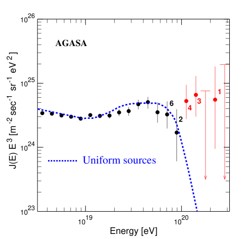
Figure 4: Observed energy spectrum of cosmic rays extending beyond the GZK cutoff [17].

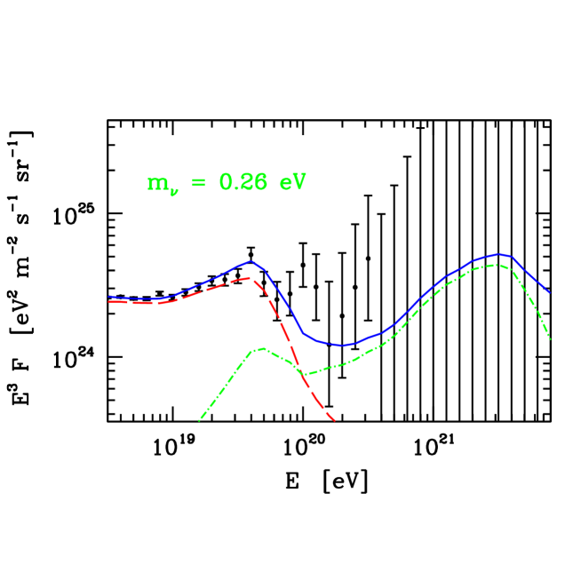
Figure 5: Energy spectrum of cosmic rays predicted from Z-bursts of extragalactic cosmic neutrinos and relic neutrinos with mass $m_{\nu}=0.26\ \mbox{eV}$ [22].

The detection of the relic neutrinos is an outstanding problem. It has been suggested that this may be possible by means of ‘Z-bursts’ (fig. 3), which result from the resonant annihilation of ultrahigh energy cosmic neutrinos (UHEC$\nu$s) with relic neutrinos [18, 19]. On resonance, the annihilation cross section is enhanced by several orders of magnitude. In the rest system of the massive relic neutrinos the resonance condition is fullfilled for the incident neutrino energy

$$E^{res}_{\nu}={M_{Z}^{2}\over 2m_{\nu}}=4.2\times 10^{21}\ \mbox{eV}\left(m_{\nu}[\mbox{eV}]\right)^{-1}\;,$$ (17)

where $M_{Z}$ is the Z-boson mass. For neutrino masses ${\cal O}(\mbox{eV})$ these energies are remakably close to the highest energy cosmic rays observed.

Z-bursts are indeed a possible explanation [20, 21] of the observed excess at energies above the Greisen-Zatsepin-Kuzmin (GZK) cutoff $E_{GZK}=4\times 10^{19}$ GeV (fig. 4). In a detailed study of extragalactic neutrinos a quantitive description of the data (fig. 5) is obtained for neutrino masses [22],

$$m_{\nu}=0.26^{+0.20}_{-0.14}\ \mbox{eV}\;.$$ (18)

In fig. 5 the first bump at $E=4\times 10^{19}$ GeV represents protons produced at higher energies and accumulated just above the GZK cutoff. The second bum at $E=3\times 10^{21}$ eV reflects the Z-burst.

A confirmation of the Z-burst hypothesis would prove the existence of relic neutrinos and at the same time provide an absolute neutrino mass measurement!

3 Weyl-, Dirac- and Majorana-Neutrinos

3.1 C, P and CP

The standard model is a chiral gauge theory, i.e. left- and right-handed fields have different electroweak interactions. Left-handed quarks and leptons are doublets with respect to the gauge group SU(2) of the weak interactions, whereas right-handed quarks and leptons are singlets,

$$q_{L}=\left(\begin{array}[]{c}u_{L}\\ d_{L}\end{array}\right)\;,\quad u_{R}\;,\quad d_{R}\;,\quad l_{L}=\left(\begin{array}[]{c}\nu_{L}\\ e_{L}\end{array}\right)\;,\quad e_{R}\;.$$ (19)

For massless particles helicity and chirality are identical. The chirality transformation corresponds to a multiplication of the Dirac spinor by $\gamma_{5}$,

$$\gamma_{5}\psi_{L}(t,\vec{x})=-\psi_{L}(t,\vec{x})\;,\quad\gamma_{5}\psi_{R}(t,\vec{x})=+\psi_{R}(t,\vec{x})\;.$$ (20)

Since left- and right-handed fields, which have different gauge interactions, also have opposite chiralities, the standard model is called a chiral gauge theory.

For the standard model, the transformation properties of the fields under $C$, $P$ and $C\!P$ are of fundamental importance. Charge conjugation and parity are defined as

$$C:\qquad\psi(t,\vec{x})\rightarrow\psi^{C}(t,\vec{x}) = C\overline{\psi}^{T}\!(t,\vec{x})\;,$$ (21)

$$P:\qquad\psi(t,\vec{x})\rightarrow\psi^{P}(t,\vec{x}) = P\psi(t,-\vec{x})\;.$$ (22)

Here $C=i\gamma_{2}\gamma_{0}$, $\overline{\psi}=\psi^{\dagger}\gamma_{0}$ and $P=\gamma_{0}$. For simplicity, we have set possible phase factors in the definition of $C$ and $P$ equal to 1. One easily verifies that $C$ and $P$ transformations change chirality,

$$\gamma_{5}\psi^{P}_{L}(t,\vec{x})=\gamma_{5}\gamma_{0}\psi_{L}(t,-\vec{x})=+\psi_{L}^{P}(t,\vec{x})\;,$$ (23)

$$\gamma_{5}\psi^{C}_{L}(t,\vec{x})=\gamma_{5}i\gamma_{2}\psi^{*}_{L}(t,\vec{x})=+\psi_{L}^{C}(t,\vec{x})\;.$$ (24)

Hence, parity and charge conjugated left-handed fermions are right-handed and vice versa.

In general, a Dirac fermion can be decomposed into left- and right-handed parts,

$$\psi={1+\gamma_{5}\over 2}\psi+{1-\gamma_{5}\over 2}\psi=\psi_{R}+\psi_{L}\;.$$ (25)

Parity and charge conjugation then relate these two components. However, in the standard model left- and right-handed fields have different weak interactions. For the up-quark, for instance, one has,

$$u=u_{R}+u_{L}\;,\quad u_{L}=q_{L}^{1}\;,$$ (26)

i.e. $u_{L}$, the left-handed partner of $u_{R}$, changes under SU(2) gauge transformations. Hence, one cannot define $P$ and $C$ transformations which commute with the electroweak gauge symmetries. For neutrinos the situation is even worse, since right-handed neutrinos don’t even exist in the minimal standard model! Only the $C\!P$ transformation is well defined,

$$C\!P:\qquad\psi(t,\vec{x})\rightarrow\psi^{CP}\!(t,\vec{x})=C\!P\overline{\psi}^{T}\!(t,-\vec{x})\;,$$ (27)

since it does not change chirality,

$$\gamma_{5}\psi^{CP}_{L}=-\psi^{CP}_{L}\;,\quad\gamma_{5}\psi^{CP}_{R}=+\psi^{CP}_{R}\;.$$ (28)

Hence, in principle, $C\!P$ could be a symmetry of the standard model.

Neutrinos are the quanta of the left-handed field $\nu_{L}(x)$. Neutrino states are created by the field operator which has the mode expansion,

$$\nu_{L}(x)=\int d\bar{p}\left(b(p)u_{L}(p)e^{-ip\cdot x}+d^{\dagger}(p)v_{L}(p)e^{ip\cdot x}\right)\;,$$ (29)

where $d\bar{p}=d^{3}p/[(2\pi)^{3}2E]$. The operators $b^{\dagger}(p)$ and $d^{\dagger}(p)$ create from the vacuum neutrino and antineutrino states, respectively,

$$|\nu;p\rangle=b^{\dagger}(p)|0\rangle\;,\quad|\bar{\nu};p\rangle=d^{\dagger}(p)|0\rangle\ \;.$$ (30)

The operators for energy, momentum, helicity and lepton number are given by (cf. [23]),

$$P_{\mu} = {i\over 2}\int d^{3}x:\psi^{\dagger}\vbox{\halign{#\cr$\mathord{\leftarrow}\mkern-6.0mu\cleaders\hbox{$\mkern-2.0mu\mathord{-}\mkern-2.0mu$}\hfill\mkern-6.0mu\mathord{\rightarrow}$\crcr\kern-1.0pt\nointerlineskip\cr$\hfil\displaystyle{\partial_{\mu}}\hfil$\crcr}}\psi:\ =\int d\bar{p}\ p_{\mu}\left(b^{\dagger}(p)b(p)+d^{\dagger}(p)d(p)\right)\;,$$ (33)

$$\vec{\Sigma}\cdot\vec{P} = {i\over 2}\int d^{3}x:\psi^{\dagger}\sigma^{i}\vbox{\halign{#\cr$\mathord{\leftarrow}\mkern-6.0mu\cleaders\hbox{$\mkern-2.0mu\mathord{-}\mkern-2.0mu$}\hfill\mkern-6.0mu\mathord{\rightarrow}$\crcr\kern-1.0pt\nointerlineskip\cr$\hfil\displaystyle{\partial^{i}}\hfil$\crcr}}\psi:\ =-\int d\bar{p}\ E\left(b^{\dagger}(p)b(p)-d^{\dagger}(p)d(p)\right)\;,$$ (36)

$$L = \int d^{3}x:\psi^{\dagger}\psi:\ =\int d\bar{p}\left(b^{\dagger}(p)b(p)-d^{\dagger}(p)d(p)\right)\;;$$ (37)

here $\sigma^{i}={i\over 2}\epsilon_{ijk}\gamma^{j}\gamma^{k}$. Using the usual anticommutation relations for creation and annihilation operators one reads off from eqs. (33)-(37),

$$P_{\mu}|\nu;p\rangle=p_{\mu}|\nu;p\rangle\;,\quad{\vec{\Sigma}\cdot\vec{P}\over E}|\nu;p\rangle=-|\nu;p\rangle=-L|\nu;p\rangle\;,$$ (38)

$$P_{\mu}|\bar{\nu};p\rangle=p_{\mu}|\bar{\nu};p\rangle\;,\quad{\vec{\Sigma}\cdot\vec{P}\over E}|\bar{\nu};p\rangle=+|\bar{\nu};p\rangle=-L|\bar{\nu};p\rangle\;,$$ (39)

i.e. the helicity (lepton number) of antineutrinos is positive (negative). Note, that helicity and lepton number always have opposite sign.

3.2 Mass generation in the standard model

Since the standard model is a chiral gauge theory quark and lepton masses can only be generated via spontaneous symmetry breaking. Starting from the Yukawa interactions

$${\cal L}_{Y}^{(q,e)}=h_{uij}\overline{q}_{Li}u_{Rj}H_{1}+h_{dij}\overline{q}_{Li}d_{Rj}H_{2}+h_{eij}\overline{l}_{Li}e_{Rj}H_{2}\;+\;h.c.\;,$$ (40)

the vacuum expectation values of the Higgs fields, $\left\langle H\right\rangle_{1}=v_{1}$ and $\left\langle H\right\rangle_{2}=v_{2}$, lead to the mass terms,

$${\cal L}_{M}^{(q,e)}=m_{uij}\overline{u}_{Li}u_{Rj}+m_{dij}\overline{d}_{Li}d_{Rj}+m_{eij}\overline{e}_{Li}e_{Rj}\;+\;h.c.\;,$$ (41)

with the mass matrices for up-quarks, down-quarks and charged leptons,

$$m_{u}=h_{u}v_{1}\;,\quad m_{d}=h_{d}v_{2}\;,\quad m_{e}=h_{e}v_{2}\;.$$ (42)

The mass matrices are diagonalized by bi-unitary transformations,

$$V^{(u)\dagger}m_{u}\widetilde{V}^{(u)}=m_{u}^{diag}\;,\quad V^{(d)\dagger}m_{d}\widetilde{V}^{(d)}=m_{d}^{diag}\;,\quad V^{(e)\dagger}m_{e}\widetilde{V}^{(e)}=m_{e}^{diag}\;,\quad$$ (43)

with $V^{(u)\dagger}V^{(u)}=1$, etc. , which also define the transition from weak eigenstates $\psi_{L\alpha}$, $\psi_{R\alpha}$ to mass eigenstates $\psi_{Li}$, $\psi_{Ri}$,

$$u_{L\alpha}=V^{(u)}_{\alpha i}u_{Li}\;,\quad d_{L\alpha}=V^{(d)}_{\alpha i}d_{Li}\;,\ldots,e_{R\alpha}=\widetilde{V}^{(e)}_{\alpha i}e_{Ri}\;.$$ (44)

Since in general the transformation matrices are different for up- and down-quarks one obtains a mixing between mass eigenstates in the charged current (CC) weak interactions,

$${\cal L}^{(q)}_{EW} = -{g\over\sqrt{2}}\sum_{\alpha}\overline{u}_{L\alpha}\gamma^{\mu}d_{L\alpha}\ W^{+}_{\mu}\ +\ldots$$ (45)

$$= -{g\over\sqrt{2}}\sum_{i,j}\overline{u}_{Li}\gamma^{\mu}V_{ij}d_{Lj}\ W^{+}_{\mu}\ +\ldots\;,$$

where $V_{ij}=V^{(u)\dagger}_{i\alpha}V^{(d)}_{\alpha j}$ is the familiar CKM mixing matrix. In general the Yukawa couplings are complex; hence, also the CKM matrix is complex, which leads to $C\!P$ violation in weak interactions.

Without right-handed neutrinos, weak and mass eigenstates can always be chosen to coincide for leptons. As a consequence, there is no mixing in the leptonic charged current,

$${\cal L}^{(l)}_{EW}=-{g\over\sqrt{2}}\sum_{\alpha}\overline{e}_{Li}\gamma^{\mu}\nu_{Li}\ W^{-}_{\mu}\ +\ldots\;,$$ (46)

and electron-, muon- and tau-number are separately conserved. On the contrary, in the quark sector only the total baryon number is conserved.

3.3 Neutrino masses and mixings

The simplest, and theoretically favoured, way to introduce neutrino masses makes use of right-handed neutrinos $\nu_{R}$. This allows additional Yukawa couplings and a Majorana mass term,

$${\cal L}_{Y}^{(\nu)}=h_{\nu ij}\overline{l}_{Li}\nu_{Rj}H_{1}+{1\over 2}M_{ij}\overline{\nu_{R}^{c}}_{i}\nu_{Rj}\;+\;h.c.$$ (47)

The Yukawa interaction defines the quantum numbers of the right-handed neutrino: it carries lepton number, which is a global charge, but no colour, weak isospin or hypercharge, which are gauge quantum numbers. Hence, a Majorana mass term is allowed for the right-handed neutrinos, consistent with the gauge symmetries of the theory. It is very important that these masses are not generated by the Higgs mechanism and can therefore be much larger than ordinay quark and lepton masses. This leads to light neutrino masses via the seesaw mechanism [24].

The Yukawa interaction which couples left-handed and right-handed neutrinos yields after spontaneous symmetry breaking the Dirac neutrino mass matrix $m_{D}=h_{\nu}v_{1}$, so that the complete mass terms are given by

$${\cal L}_{M}^{(\nu)}=m_{Dij}\overline{\nu_{L}}_{i}\nu_{Rj}+{1\over 2}M_{ij}\overline{\nu_{R}^{c}}_{i}\nu_{Rj}\;+\;h.c.$$ (48)

In order to obtain the mass eigenstates one has to perform a unitary transformation. Using $\overline{\nu_{L}}m_{D}\nu_{R}=\overline{\nu_{R}^{c}}m_{D}^{T}\nu_{L}^{c}$, the mass terms can be written in matrix form

$${\cal L}_{M}^{(\nu)}={1\over 2}\left(\begin{array}[]{cc}\overline{\nu_{L}}&\overline{\nu_{R}^{c}}\end{array}\right)\left(\begin{array}[]{cc}0&m_{D}\\ m_{D}^{T}&M\end{array}\right)\left(\begin{array}[]{c}\nu_{L}^{c}\\ \nu_{R}\end{array}\right)\;+\;h.c.$$ (49)

The unitary matrix which diagonalizes this mass matrix is easily constructed as power series in $\xi=m_{D}/M$. Up to terms ${\cal O}(\xi^{3})$ one obtains

$$\left(\begin{array}[]{c}\nu_{L}\\ \nu_{R}^{c}\end{array}\right)=\left(\begin{array}[]{cc}1-{1\over 2}\xi\xi^{\dagger}&\xi\\ -\xi^{\dagger}&1-{1\over 2}\xi\xi^{\dagger}\end{array}\right)\left(\begin{array}[]{c}L\\ R^{c}\end{array}\right)\;.$$ (50)

In terms of the new left- and right-handed fields, $L$ and $R$, the mass matrix is diagonal,

$${\cal L}_{M}^{(\nu)}={1\over 2}\left(\begin{array}[]{cc}\overline{L}&\overline{R^{c}}\end{array}\right)\left(\begin{array}[]{cc}m_{\nu}&0\\ 0&M\end{array}\right)\left(\begin{array}[]{c}L^{c}\\ R\end{array}\right)\;+\;h.c.$$ (51)

Here the mass matrix $m_{\nu}$ is given by

$$m_{\nu}=-m_{D}{1\over M}m_{D}^{T}\;.$$ (52)

This is the famous seesaw mass relation [25]. With $M\gg m_{D}$, one obviously has $m_{\nu}\ll m_{D}$. As an example, consider the case of just one generation. Choosing for $m_{D}$ the largest know fermion mass, $m_{D}\sim m_{t}\sim 100$ GeV, and for $M$ the unification scale of unified theories, $M\sim 10^{15}$ GeV, one finds $m_{\nu}\sim 10^{-2}$ eV, which is precisely in the range of present experimental indications for neutrino masses.

$m_{\nu}$ and $M$ are the mass matrices of the light neutrinos and their heavy partners, respectively. The corresponding mass eigenstates are Majorana fermions,

$$\nu=L+L^{c}=\nu^{c}\;,\quad N=R^{c}+R=N^{c}\;.$$ (53)

$L,R^{c}$ and $L^{c},R$ are the corresponding left- and right-handed components,

$$L={1-\gamma_{5}\over 2}\nu\;,\quad R^{c}={1-\gamma_{5}\over 2}N\;,\quad\mbox{etc.}$$ (54)

In terms of the Majorana fields the mass terms read,

$$\ {\cal L}_{M}^{(\nu)} = {1\over 2}\overline{\nu}m_{\nu}{1+\gamma_{5}\over 2}\nu+{1\over 2}\overline{N}m_{\nu}{1+\gamma_{5}\over 2}N\;+\;h.c.$$ (55)

$$= {1\over 2}\overline{\nu}\left(\mbox{Re}\{m_{\nu}\}+i\mbox{Im}\{m_{\nu}\}\gamma_{5}\right)\nu+{1\over 2}\overline{N}\left(\mbox{Re}\{M\}+i\mbox{Im}\{M\}\gamma_{5}\right)N\;.$$

Note, that in general the mass matrices have real and imaginary parts. This is a consequence of complex Yukawa couplings and a possible source of $C\!P$ violation.

The mode expansion of the Majorana field operator reads,

$$\nu(x)=\nu^{c}(x)=\int d\bar{p}\sum_{i=1}^{2}\left(a_{i}(p)u_{i}(p)e^{-ip\cdot x}+a^{\dagger}_{i}(p)v_{i}(p)e^{ip\cdot x}\right)\;,$$ (56)

where $u_{i}(p)$ and $v_{i}(p)=u^{c}_{i}(p)$ are now solutions of the massive Dirac equation. In the massless case the connection with the left-handed neutrino field (29) is very simple,

$$a_{1}(p)=b(p)\;,\quad a_{2}(p)=d(p)\;,\quad u_{1}(p)=u_{L}(p)\;,\quad u_{2}(p)=v_{L}^{c}(p)\;,$$ (57)

i.e. the two spin states of the Majorana neutrino are identical with the neutrino and antineutrino states. In the massless case these states carry different lepton number, which is conserved. For massive Majorana neutrinos lepton number is violated by the Majorana mass term which couples the two polarization states.

So far we have only discussed the simplest version of the seesaw mechanism. Additional Higgs fields also lead to a direct mass term for the left-handed neutrinos [26]. In principle, neutrino masses could also be generated by radiative corrections. This is a possible alternative to the seesaw mechanism. Particularly attractive are supersymmetric models with broken R-parity [27], which lead to signatures testable at colliders.

Neutrino masses imply mixing in the leptonic charged current. If the neutrino mass matrix is diagonalized by the unitary matrix $U^{(\nu)}$,

$$U^{(\nu)\dagger}m_{\nu}U^{(\nu)*}=-\left(\begin{array}[]{ccc}m_{1}&0&0\\ 0&m_{2}&0\\ 0&0&m_{3}\end{array}\right)\;,$$ (58)

the mixing matrix $U$ appears in the charged current,

$${\cal L}^{(l)}_{EW}=-{g\over\sqrt{2}}\sum_{ij}\overline{e}_{Li}\gamma^{\mu}U_{ij}\nu_{Lj}\ W^{-}_{\mu}\ +\ldots\;,$$ (59)

where

$$U_{ij}=U^{(e)\dagger}_{i\alpha}U^{(\nu)}_{\alpha j}\;.$$ (60)

$e$-, $\mu$- and $\tau$-number are now no longer separately conserved. The mixing matrix is frequently written in the following form,

$$U=\left(\begin{array}[]{ccc}U_{e1}&U_{e2}&U_{e3}\\ U_{\mu 1}&U_{\mu 2}&U_{\mu 3}\\ U_{\tau 1}&U_{\tau 2}&U_{\tau 3}\end{array}\right)\;,$$ (61)

and can be expressed in the standard way as product of three rotation in the 12-, 13- and 23-planes,

$$U=\left(\begin{array}[]{ccc}1&0&0\\ 0&c_{23}&s_{23}\\ 0&-s_{23}&c_{23}\end{array}\right)\left(\begin{array}[]{ccc}c_{13}&0&s_{13}e^{-i\delta}\\ 0&1&0\\ -s_{13}e^{i\delta}&0&c_{13}\end{array}\right)\left(\begin{array}[]{ccc}c_{12}&s_{12}&0\\ -s_{12}&c_{12}&0\\ 0&0&1\end{array}\right)\;.$$ (62)

As we shall see in the next section, present data are consistent with a small value of $s_{13}$. The $3\times 3$ mixing matrix then becomes a product of two $2\times 2$ matrices describing mixing between the first and second, and the second and third generations, respectively. This very simple mixing pattern appears to be sufficient to account for the solar and the atmospheric neutrino deficits.

4 Neutrino Oscillations

In recent years there has been a wealth of experimental data in neutrino physics, and we can look forward to important new results also in the coming years. The present situation is summarized in fig. 6 which is taken from the review of particle physics. The latest most important result is the first data from SNO which we shall discuss in section 4.3. Detailed discussions of neutrino oscillations and references can be found in the reviews [29]-[32].

4.1 Oscillations in vacuum

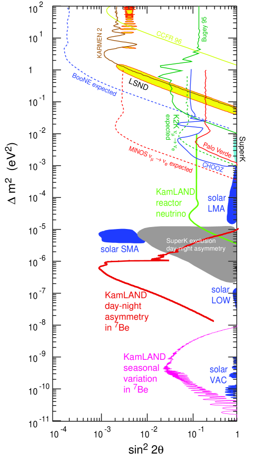
Figure 6: The most important exclusion limits as well as preferred parameter regions from neutrino oscillation experiments assuming two-flavour oscillatons [28].

Neutrino oscillations [33, 34] are a very intriguing quantum mechanical effect similar to the well known oscillations between $K^{0}$- and $\overline{K^{0}}$-mesons. They occur because of the mixing in the charged weak current discussed in the previous section. The neutral and charged current weak interactions of neutrinos are described by the lagrangian

$${\cal L}_{EW}=-\sum_{\alpha,i}\left\{{g\over 2\cos{\Theta_{W}}}\overline{\nu}_{L\alpha}\gamma^{\mu}\nu_{L\alpha}\ Z_{\mu}+{g\over\sqrt{2}}\overline{e}_{L\alpha}\gamma^{\mu}U_{\alpha i}\nu_{Li}\ W^{-}_{\mu}\ +h.c.\right\}\;,$$ (63)

where the fields $e_{L\alpha}$, $\alpha=1\ldots 3$, represent the mass eigenstates of electron, muon and tau, and the fields $\nu_{Li}$, $i=1\ldots n\geq 3$, correspond to neutrino mass eigenstates. Hence, the charged lepton $e_{\alpha}$ couples to the neutrino flavour eigenstate $\nu_{\alpha}$, which is a linear superposition of mass eigenstates,

$$\nu_{\alpha}=\sum_{i}U^{*}_{\alpha i}\nu_{i}\;.$$ (64)

Figure 7: Neutrino production, propagation and absorption.

Here $\nu_{\alpha}$ and $\nu_{i}$ are spinors in flavour space, and $U$ is a $n\times n$ unitary matrix. Three linear combinations of mass eigenstates have weak interactions, and are therefore called active, whereas $n-3$ linear combinations are sterile, i.e. they don’t feel the weak force. In the case $n=4$, for instance, the sterile neutrino is given by

$$\nu_{s}=\sum_{i}U^{*}_{4i}\nu_{i}\;.$$ (65)

In the following we will restrict ourselves to the case of three active neutrinos and shall not discuss the positive signature for oscillations from the LSND experiment [35] at Los Alamos, which would require the existence of a sterile neutrino.

Neutrinos are relativistic particles whose propagation is described by the Dirac equation. Consider now a neutrino beam propagating in z-direction from a source at $z=0$ to a detector at $z=L$. The probability for neutrino oscillation is usually derived by considering first the time evolution of a spatially homogeneous state. Some hand waving arguments are then needed to obtain the physically relevant probability for oscillations in space, which, with lack of fortune, can also give the wrong result. As pointed out by Stodolsky, all this confusion can be avoided by realizing that the system corresponds to a stationary state [36, 37] which is completely characterized by the energy spectrum of the beam. For simplicity, we first consider the case of fixed energy $E$. The wave packet description of neutrino oscillations is discussed in ref. [38].

Neglecting the mixing between neutrinos and antineutrinos, which is suppressed by $\left(m_{i}/E\right)^{2}$, the hamiltonian of the system reads in the mass eigenstate basis,

$$H_{0} = \left(\begin{array}[]{ccc}\sqrt{\hat{p}^{2}+m_{1}^{2}}&0&0\\ 0&\sqrt{\hat{p}^{2}+m_{2}^{2}}&0\\ 0&0&\sqrt{\hat{p}^{2}+m_{3}^{2}}\end{array}\right)$$ (69)

$$\simeq \left(\begin{array}[]{ccc}\hat{p}+{m_{1}^{2}\over 2\hat{p}}&0&0\\ 0&\hat{p}+{m_{2}^{2}\over 2\hat{p}}&0\\ 0&0&\hat{p}+{m_{3}^{2}\over 2\hat{p}}\end{array}\right)\;;$$ (73)

here $\hat{p}$ is the momentum operator conjugate to the $z$-coordinate, and we have assumed that the relevant eigenvalues are much larger than the neutrino masses $m_{i}$. To describe the neutrino oscillation $\nu_{\alpha}\rightarrow\nu_{\beta}$ we have to find an energy eigenstate,

$$H_{0}\nu_{E}^{(\alpha)}(z)=E\nu_{E}^{(\alpha)}(z)\;,$$ (74)

which satisfies the boundary condition

$$\nu_{E}^{(\alpha)}(0)=\nu_{\alpha}\;.$$ (75)

The solution reads

$$\nu_{E}^{(\alpha)}(z)=\sum_{i}U^{*}_{\alpha i}\nu^{(i)}_{p_{i}}(z)\;,$$ (76)

where the momentum eigenstates are given by

$$\nu^{(i)}_{p_{i}}(z)=e^{ip_{i}z}\nu_{i}\;,$$ (77)

with $p_{i}\simeq E-m_{i}^{2}/(2E)$. For the dependence of the wave function $\nu_{E}^{(\alpha)}(z)$ on the $z$-coordinate one then obtains,

$$\nu_{E}^{(\alpha)}(z)=\sum_{i}U^{*}_{\alpha i}e^{ip_{i}z}\nu_{i}\;.$$ (78)

Using the unitarity of the mixing matrix, $U^{\dagger}U=1$, this yields for the flavour transition probability between the source at $z=0$ and the detector at $z=L$,

$$P(\nu_{\alpha}\rightarrow\nu_{\beta}) = |\nu^{\dagger}_{\beta}\nu^{(\alpha)}_{E}(L)|^{2}$$ (79)

$$= \delta_{\beta\alpha}+\sum_{i,j}U_{\beta i}U_{\alpha i}^{*}U_{\beta j}^{*}U_{\alpha i}\left(e^{-i\Delta m^{2}_{ij}{L\over 2E}}-1\right)\;,$$

where

$$\Delta m^{2}_{ij}=m_{i}^{2}-m_{j}^{2}\;.$$ (80)

Terms with $i=j$ do not contribute in the sum (79), and a very useful form of transition probability is

$$P(\nu_{\alpha}\rightarrow\nu_{\beta})=\delta_{\alpha\beta} - 4\sum_{i>j}\mbox{Re}\left(U_{\alpha i}^{*}U_{\beta i}U_{\alpha j}U_{\beta j}^{*}\right)\sin^{2}{\left(\Delta m^{2}_{ij}{L\over 4E}\right)}$$ (81)

$$+ 2\sum_{i>j}\mbox{Im}\left(U_{\alpha i}^{*}U_{\beta i}U_{\alpha j}U_{\beta j}^{*}\right)\sin^{2}{\left(\Delta m^{2}_{ij}{L\over 2E}\right)}\;.$$

Note the different oscillation lengths of the real and imaginary parts. In the realistic case of a neutrino beam with some energy spectrum $\rho(E)$, one has to integrate over energy,

$$\bar{P}(\nu_{\alpha}\rightarrow\nu_{\beta})=\int dE\rho(E)P(\nu_{\alpha}\rightarrow\nu_{\beta})\;.$$ (82)

All patterns of neutrino oscillations including $C\!P$ violation are described by the master formula (81). Let us discuss some of its properties:

• The dependence on $L$ shows the expected oscillatory behaviour, which is an interference effect and dissapears for $\Delta m^{2}_{ij}=0$.

• Due to the unitarity of the mixing matrix $U$ the total flux of neutrinos is conserved,

  $$\sum_{\beta}P(\nu_{\alpha}\rightarrow\nu_{\beta})=\sum_{i}|U_{\alpha i}|^{2}=1\;.$$ (83)

• In the simplest case of only 2 flavours $(\alpha,\beta=e,\mu)$ only one term contributes in the sum of (81). The unitarity of the mixing matrix $U$ then implies $(i=2,j=1)$, $U_{\alpha 2}^{*}U_{\beta 2}U_{\alpha 1}U_{\beta 1}^{*}=-|U_{\alpha 2}|^{2}|U_{\beta 2}|^{2}$. This yields for the transition probability

  $$P(\nu_{\alpha}\rightarrow\nu_{\beta})=4|U_{\alpha 2}|^{2}|U_{\beta 2}|^{2}\sin^{2}{\left(\Delta m^{2}{L\over 4E}\right)}\;,$$ (84)

  where $\Delta m^{2}=m_{2}^{2}-m_{1}^{2}$. The unitary $2\times 2$ mixing matrix can be parametrized in the standard way in terms of 1 rotation angle and 3 phases,

  $$U=\left(\begin{array}[]{cc}e^{i\phi_{1}}\cos{\Theta_{0}}&e^{i(\phi_{2}-\phi_{3})}\sin{\Theta_{0}}\\ -e^{i(\phi_{1}+\phi_{3})}\sin{\Theta_{0}}&e^{i\phi_{2}}\cos{\Theta_{0}}\end{array}\right)\;.$$ (85)

  With $4|U_{\alpha 2}|^{2}|U_{\beta 2}|^{2}=\sin^{2}{2\Theta_{0}}$ one then reads off from eq. (84) the standard formula for the transition probability in the case of 2 flavours,

  $$P(\nu_{\alpha}\rightarrow\nu_{\beta})=\sin^{2}{2\Theta_{0}}\sin^{2}{{L\over L_{vac}}}\;,$$ (86)

  with the vacuum oscillation length

  $$L_{vac} = {4E\over\Delta m^{2}}={2\over\Delta p}$$ (87)

  $$\simeq 1.27\ \mbox{km}\left({E[\mbox{GeV}]\over\Delta m^{2}[\mbox{eV}^{2}]}\right)\;.$$

  For fast oscillations, i.e. large oscillation phase, averaging over the energy resolution of the detector and the distance $L$ according to the uncertainty of the production point, yields the average transition probability,

  $$\overline{P(\nu_{\alpha}\rightarrow\nu_{\beta})}={1\over 2}\sin^{2}{2\Theta_{0}}\;.$$ (88)

  In disappearance experiments one measures the survival probability $P(\nu_{\alpha}\rightarrow\nu_{\alpha})$ which is directly related to the transition probability,

  $$P(\nu_{\alpha}\rightarrow\nu_{\alpha}) = 1-P(\nu_{\alpha}\rightarrow\nu_{\beta})$$ (89)

  $$= 1-4|U_{\alpha 2}|^{2}(1-|U_{\alpha 2}|^{2})\sin^{2}{\left(\Delta m^{2}{L\over 4E}\right)}\;.$$

• Particularly interesting is the case of three hierarchical neutrinos, $m_{1}^{2}\ll m_{2}^{2}\ll m_{3}^{2}$. Suppose that $\Delta m_{31}^{2}L/(4E)={\cal O}(1)$, and correspondingly $\Delta m_{21}^{2}L/(4E)\ll 1$. From eq. (81) one then obtains

  $$P(\nu_{\alpha}\rightarrow\nu_{\beta}) \simeq -4\mbox{Re}\left(U_{\alpha 3}^{*}U_{\beta 3}U_{\alpha 2}U_{\beta 2}^{*}+U_{\alpha 3}^{*}U_{\beta 3}U_{\alpha 1}U_{\beta 1}^{*}\right)\sin^{2}{\left(\Delta m^{2}_{31}{L\over 4E}\right)}$$ (90)

  $$= 4|U_{\alpha 3}|^{2}|U_{\beta 3}|^{2}\sin^{2}{\left(\Delta m^{2}_{31}{L\over 4E}\right)}\;.$$

  Note, that this result is completely analogous to the two-flavour case; only the large mass difference matters.

• The sensitivity of an oscillation experiment with respect to the neutrino mass difference $\Delta m^{2}$ is determined by the neutrino energy $E$ and the oscillation length $L$. Oscillations become visible for mass differences above $\Delta m^{2}L/(4E)\simeq 1$. In the appropriate units of energy and length this condition reads

  $$\Delta m^{2}[\mbox{eV}^{2}]\simeq{E[\mbox{GeV}]\over L[\mbox{km}]}\;.$$ (91)

  Relevant examples are given in table 1.

  	$L$[km]	$E$[GeV]	$\Delta m^{2}$ [eV2]
  accelerator (short baseline)	0.1	1	10
  reactor	0.1	$10^{-3}$	$10^{-2}$
  accelerator (long baseline)	$10^{3}$	10	$10^{-2}$
  atmospheric	$10^{4}$	1	$10^{-4}$
  solar	$10^{8}$	$10^{-3}$	$10^{-11}$

  Table 1: The approximate reach in $\Delta m^{2}$ of different oscillation experiments.

• In the past the sensitivity of neutrino oscillation experiments has been mostly displayed in the ($\Delta m^{2}$, $\sin^{2}{2\Theta}$) plane. Obviously, this parametrization covers only half of the parameter space. More appropriate are the variables ($\Delta m^{2}$, $\tan^{2}{\Theta}$), which is particularly important for oscillations in matter [39].

• The measurement of magnitude and sign of $C\!P$ violation in neutrino oscillations would be of fundamental importance. One $C\!P$ violating observable is the asymmetry

  $$\Delta_{e\mu}=P(\nu_{e}\rightarrow\nu_{\mu})-P(\bar{\nu}_{e}\rightarrow\bar{\nu}_{\mu})\;.$$ (92)

  Using $C\!P\!T$ invariance and the unitarity of the mixing matrix one easily verifies that in the case of three neutrino flavours the three possible asymmetries are all equal,

  $$\Delta_{e\mu}=\Delta_{\mu\tau}=\Delta_{\tau e}\;.$$ (93)

  From the master formula (81) one reads off,

  $$\Delta_{\alpha\beta}=4\sum_{i>j}\mbox{Im}\left(U_{\alpha i}^{*}U_{\beta i}U_{\alpha j}U_{\beta j}^{*}\right)\sin^{2}{\left(\Delta m^{2}_{ij}{L\over 2E}\right)}\;.$$ (94)

  The product of mixing matrices is completely antisymmetric in the flavour indices,

  $$\mbox{Im}\left(U_{\alpha i}^{*}U_{\beta i}U_{\alpha j}U_{\beta j}^{*}\right)=\widetilde{\epsilon}_{\alpha\beta}\widetilde{\epsilon}_{ij}J_{l}\;,$$ (95)

  where $\widetilde{\epsilon}_{ab}=\sum_{c=1}^{3}\epsilon_{abc}$ and $J_{l}$ is the leptonic Jarlskog parameter. For quarks one finds for the corresponding quantity $J_{q}\sim 10^{-5}$. Due to the large neutrino mixings $J_{l}$ turns out to be much larger, which gives hope to observe $C\!P$ violating effects in future superbeam experiments and at a neutrino factory [40].

4.2 Oscillations in matter

In vacuum, neutrino oscillation probabilities are bounded by the mixing angle, $P\leq\sin^{2}{2\Theta_{0}}$. Hence, for small mixing angles transition probabilites are small. In matter, a resonance enhancement of neutrino oscillations can take place and transition probabilities can be maximal even for small vacuum mixing angles $-$ this is the Mikheyev-Smirnov-Wolfenstein effect [41].

The matter enhancement of oscillations is a coherent effect, due to elastic forward scattering of neutrinos with negligible momentum transfer. The effect can be described by the propagation of the neutrinos in an approximately constant potential generated by the exchange of $W$-bosons (fig. 8),

$$L_{CC}=-2\sqrt{2}G_{F}\overline{e_{L}}\gamma^{\mu}\nu_{Le}\overline{\nu_{L}}\gamma_{\mu}e_{L}\;.$$ (96)

The corresponding $Z$-exchange does not distinguish between $\nu_{e}$, $\nu_{\mu}$ and $\nu_{\tau}$, and therefore it has no influence on neutrino oscillations.

Figure 8: Neutrino interaction with matter via charged and neutral currents.

After a Fierz-transformation one obtains from eq. (96),

$$L_{CC}=-2\sqrt{2}G_{F}\overline{\nu_{Le}}\gamma^{\mu}\nu_{Le}\overline{e_{L}}\gamma_{\mu}e_{L}\;.$$ (97)

In order to obtain the effective potential for the neutrino propagation in matter, e.g. the interior of the sun, one has to evaluate the expectation value of the electron current in the corresponding state, i.e. the quantity $\langle\overline{e}\gamma^{\mu}(1-\gamma_{5})e\rangle$. Since no polarization vector and no spatial direction are singled out, one has

$$\langle\overline{e}\gamma^{\mu}\gamma_{5}e\rangle=0\;,\quad\langle\overline{e}\gamma^{i}e\rangle=0\;,$$ (98)

$$\langle\overline{e}\gamma^{0}e\rangle=\langle e^{\dagger}e\rangle=2n_{e}\;,$$ (99)

where $n_{e}$ is the electron number density and we have summed over electron spins.

The final lagrangian describing the propagation of neutrinos now reads (cf. (55), $m_{\nu}=m_{\nu}^{*}$),

$${\cal L}={1\over 2}\overline{\nu_{\alpha}}\left(i\hbox to0.0pt{\hbox{$\mskip 1.0mu/$}\hss}\partial\delta_{\alpha\beta}-m_{\alpha\beta}\right)\nu_{\beta}-{G_{F}\over\sqrt{2}}n_{e}\overline{\nu_{e}}\gamma^{0}\nu_{e}\;.$$ (100)

For simplicity we shall restrict ourselves in the following to the case of two flavours, i.e. $\alpha,\beta=e,\mu$. We also consider the idealized case of constant electron density. From (100) one obtains the hamiltonian

$$H=H_{0}+V\;,$$ (101)

with

$$H_{0}=\gamma^{0}\vec{\gamma}{1\over i}\vec{\partial}+\gamma^{0}m\;,\quad V=\left(\begin{array}[]{cc}\sqrt{2}G_{F}n_{e}&0\\ 0&0\end{array}\right)\;.$$ (102)

Note, that the matter induced potential has the same Lorentz structure as a static Coulomb potential. Hence, matter effects have opposite sign for neutrinos and anti-neutrinos.

The probability for flavour oscillations can now be calculated completely analogous to the case of vacuum oscillations. We again have to find a stationary state,

$$H\nu_{E}^{(\alpha)}(z)=E\nu_{E}^{(\alpha)}(z)\;,$$ (103)

which satisfies the boundary condition,

$$\nu_{E}^{(\alpha)}(0)=\nu_{\alpha}\;.$$

The free hamiltonian is known in the mass eigenstate basis (cf. (69)) where we again neglect the mixing left- and right-handed states. In the flavour basis one then has

$$H=U(\Theta_{0})H_{0}U^{\dagger}(\Theta_{0})+V\;.$$ (104)

With

$$U(\Theta_{0})=\left(\begin{array}[]{cc}\cos{\Theta_{0}}&\sin{\Theta_{0}}\\ -\sin{\Theta_{0}}&\cos{\Theta_{0}}\end{array}\right)\;,$$ (105)

the hamiltonian reads explicitely

$$H\simeq\left(\begin{array}[]{cc}\hat{p}+{m_{1}^{2}+m_{2}^{2}\over 4E}-{\Delta m^{2}\over 4E}\cos{2\Theta_{0}}+\sqrt{2}G_{F}n_{e}&{\Delta m^{2}\over 4E}\sin{2\Theta_{0}}\\ {\Delta m^{2}\over 4E}\sin{2\Theta_{0}}&\hat{p}+{m_{1}^{2}+m_{2}^{2}\over 4E}+{\Delta m^{2}\over 4E}\cos{2\Theta_{0}}\end{array}\right)\;.$$ (106)

Here $\Delta m^{2}=m_{1}^{2}-m_{2}^{2}$, and we have assumed that the relevant eigenvalues of $\hat{p}$ are $E+{\cal O}\left(m_{i}^{2}/E\right)$. It is now straightforward to diagonalize $H$, requiring

$$U^{\dagger}(\Theta)HU(\Theta)=\left(\begin{array}[]{cc}E&0\\ 0&E\end{array}\right)\;.$$ (107)

From (106) one obtains the rotation angle

$$\tan{2\Theta}={{\Delta m^{2}\over 2E}\sin{2\Theta_{0}}\over{\Delta m^{2}\over 2E}\cos{2\Theta_{0}}-\sqrt{2}G_{F}n_{e}}\;,$$ (108)

and the equation for the momentum eigenvalues

$$\left(\begin{array}[]{cc}p_{1}+{m_{1}^{2}+m_{2}^{2}\over 4E}+\sqrt{2}G_{F}n_{e}-{\Delta\over 2}&0\\ 0&p_{2}+{m_{1}^{2}+m_{2}^{2}\over 4E}+\sqrt{2}G_{F}n_{e}+{\Delta\over 2}\end{array}\right)=\left(\begin{array}[]{cc}E&0\\ 0&E\end{array}\right)\;,$$ (109)

where

$$\Delta={\Delta m^{2}\over 2E}\cos{2\Theta_{0}}-\sqrt{2}G_{F}n_{e}\;.$$ (110)

This yields the momentum eigenvalues

$$p_{1}+p_{2} = 2E-{m_{1}^{2}+m_{2}^{2}\over 2E}-\sqrt{2}G_{F}n_{e}\;,$$ (111)

$$p_{1}-p_{2} = \Delta p\ =\left(\left({\Delta m^{2}\over 2E}\cos{2\Theta_{0}}-\sqrt{2}G_{F}n_{e}\right)^{2}+\left({\Delta m^{2}\over 2E}\sin{2\Theta_{0}}\right)^{2}\right)^{1/2}\;.$$ (112)

Figure 9: Change of neutrino momentum and flavour in the sun.

The probability for flavour oscillations is again given by eq. (86), with $\Theta_{0}$ replaced by $\Theta$ and $L_{vac}$ replaced by $L_{mat}=2/\Delta p$,

$$P(\nu_{\alpha}\rightarrow\nu_{\beta}) = |\nu_{\beta}^{\dagger}\nu_{E}^{(\alpha)}(z)|^{2}$$ (113)

$$\simeq \sin^{2}{2\Theta}\sin^{2}{{L\over L_{mat}}}\;.$$

The expression (108) for the rotation angle has the typical resonance form, and maximal mixing, i.e. $\Theta=45^{o}$, is reached for

$$\sqrt{2}G_{F}n_{e}={\Delta m^{2}\over 2E}\cos{2\Theta_{0}}\;.$$ (114)

This is the MSW resonance condition. It requires in particular that ${\Delta m^{2}\over 2E}\cos{2\Theta_{0}}$ is positive. A negative sign would allow resonant oscillations for antineutrinos.

At the center of the sun the electron density is $n_{e}\sim 10^{26}/\mbox{cm}^{3}$. With $E\sim 1$ MeV, the MSW resonance condition can be fullfilled on the way out to the surface of the sun for mass differences $\Delta m^{2}\sim 10^{-5}$ eV². In the ‘adiabatic approximation’, where the oscillations are fast compared to the variation of the electron density, eqs. (111), (112) and (114) can be used at each distance $z$ from the center. The physical picture is particularly simple in the case of small mixing angle $\Theta_{0}$, where the off-diagonal terms in the hamiltonian (106) are small. The momentum of the produced electron neutrino increases, and near $z_{R}$ the transition $\nu_{e}\rightarrow\nu_{\mu}$ takes place after which the momentum stays constant (fig. 9). A more accurate calculation of the oscillation probability can be carried out similar to the treatment of the Landau-Zener effect in atomic physics [30, 32].

4.3 Comparison with experiment

We are now ready to interpret the deficit in the solar and atmospheric neutrino fluxes in terms of neutrino oscillations. In the following only a brief account of the main results will be given. More detailed discussions of the fusion processes in the sun, solar neutrino experiments, the atmospheric neutrino anomaly, reactor experiments and global fits can be found in [29]-[32].

4.3.1 Solar neutrinos

The solar energy is generated by thermonuclear reactions, in particular the $pp$ cycle and the CNO cycle, which also produce electron neutrinos. The largest neutrino flux, $\Phi_{\nu_{e}}=6.0\times 10^{10}$/[cm²s] is due to the reaction,

$$p+p\rightarrow d+e^{+}+\nu_{e}\;,$$ (115)

with a maximum neutrino energy of 0.42 MeV. Also important are the processes $e^{-}+\ ^{7}Be\rightarrow\nu_{e}+\ ^{7}Li$ with $\Phi_{\nu_{e}}=4.9\times 10^{9}$/[cm²s], $E_{\nu}=0.86$ MeV and ${}^{8}B\rightarrow\ ^{8}Be+e^{+}+\nu_{e}$, with $\Phi_{\nu_{e}}=5.0\times 10^{6}$/[cm²s], $E_{\nu}\leq 0.86$ MeV. The complete energy spectrum of solar neutrinos is summarized in fig. 10.

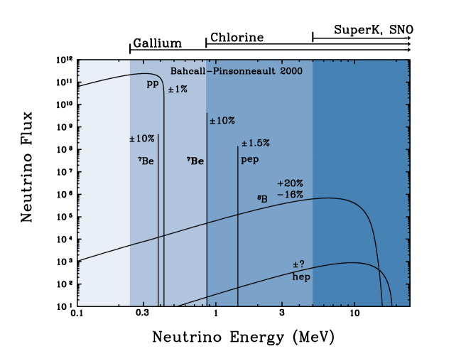
Figure 10: Solar neutrino spectrum and energy thresholds of solar neutrino experiments [42].

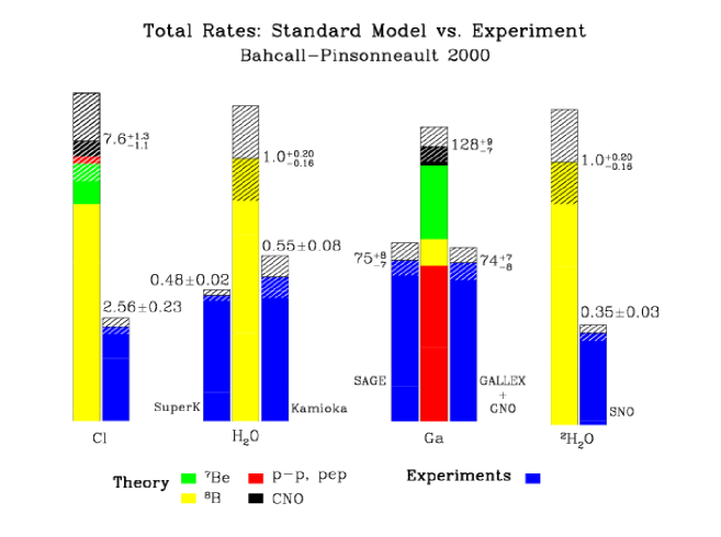
Figure 11: Theoretical flux predictions compared with experimental results; for the Cl and Ga experiments the units are SNU, for Kamiokande and Superkamiokande the ratio of measured and predicted fluxes are shown [42].

The deficit in the solar neutrino flux was discovered in radiochemical experiments. The first one was the Homestake experiment of Davis et al. based on the reaction

$$\nu_{e}+\ ^{37}Cl\rightarrow\ ^{37}Ar+e^{-}\;,$$ (116)

with an energy threshold of 0.814 MeV. Only 1/3 of the predicted flux was observed.

The GALLEX, SAGE and GNO experiments detect solar neutrinos via the reaction

$$\nu_{e}+\ ^{71}Ga\rightarrow\ ^{71}Ge+e^{-}\;.$$ (117)

Since the energy threshold is only 0.234 MeV, these experiments could see for the first time neutrinos from the dominant process (115). About 60% of the predicted flux is observed in this reaction (fig. 11).

The Kamiokande and Super-Kamiokande experiments are water Cherenkov detectors. Here the reaction,

$$\nu_{x}+e^{-}\rightarrow\nu_{x}+e^{-}\;,$$ (118)

is used to detect solar neutrinos. To suppress background only high-energy neutrinos from the ${}^{8}B$ decay, with $E>7$ GeV, are detected. As a consequence the recoil electrons are peaked in the direction of the incoming neutrino. The angular distribution of the detected electrons shows indeed a peak opposite to the direction to the sun. This clearly demonstrates the solar origin of detected neutrinos!

Figure 12: Elastic neutrino electron scattering via charged and neutral currrents.

An important step towards the final resolution of the solar neutrino problem was made by the recent results of the Sudbury Neutrino Observatory (SNO). Like in Super-Kamiokande, high-energy ${}^{8}B$ neutrinos are observed, this time in a 1000 t detector of heavy water $D_{2}O$. This allows the observation of the charged current (CC) reaction,

$$\nu_{e}+d\rightarrow p+p+e^{-}\;,$$ (119)

as well as the elastic scattering (ES),

$$\nu_{a}+e^{-}\rightarrow\nu_{a}+e^{-}\;,$$ (120)

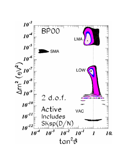
Figure 13: Two-flavour ($\nu_{e}$ to $\nu_{a}$) fit of solar neutrino data, with confidence levels 90%, 95%, 99%, 99.7% [44].

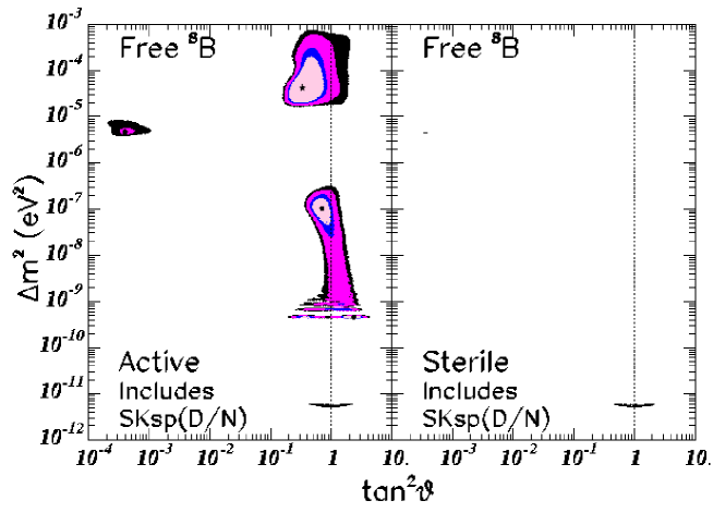
Figure 14: Comparison of two-flavour $\nu_{e}\rightarrow\nu_{a}$ and $\nu_{e}\rightarrow\nu_{s}$ fits, leaving the ${}^{8}B$ flux free [44].

which involves charged and neutral currents (fig. 12). From the CC reaction (119) one can, for the first time (!), directly determine the $\nu_{e}$ flux [43],

$$\Phi^{CC}(\nu_{e})=1.75\pm 0.07(stat)^{+0.12}_{-0.11}(syst)\pm 0.05(theo)\times 10^{6}\mbox{cm}^{-2}\mbox{s}^{-1}\;.$$ (121)

Here statistical, systematic and theoretical errors are listed separately. Under the assumption that the entire flux consists of electron neutrinos, one obtains from the ES process [43],

$$\Phi^{ES}(\nu_{e})=2.39\pm 0.34(stat)^{+0.16}_{-0.14}(syst)\times 10^{6}\mbox{cm}^{-2}\mbox{s}^{-1}\;.$$ (122)

Comparing $\Phi^{CC}$ and $\Phi^{ES}$ one concludes that with a significance of 1.6 $\sigma$ there is evidence for a non-$\nu_{e}$ component in the solar neutrino flux. Combining this with the more precise measurement of $\Phi^{ES}$ by Superkamiokande the significance increases to 3.3 $\sigma$.

Alternatively, one may assume that electron-neutrinos have partially been converted into muon- and tau-neutrinos. In this case, the flux extracted from the elastic scattering (120) should coincide with the flux of ${}^{8}B$ neutrinos. One finds [43],

$$\Phi(\nu_{a})=5.44\pm 0.99\times 10^{6}\mbox{cm}^{-2}\mbox{s}^{-1}\;,$$ (123)

in remarkable agreement with the prediction of the standard solar model!

Global fits of all solar neutrino data have been performed under different assumptions [44, 45]. Fig. 13 shows a two-flavour fit for the oscillation of $\nu_{e}$ into an active neutrino $\nu_{a}$ using the solar flux PB2000 (fig. 10). Four regions in parameter can describe the data: LMA (Large Mixing Angle MSW solution), SMA (Small Mixing Angle MSW solution), LOW (MSW solution with low $\Delta m^{2}$) and VAC (Vacuum oscillation solution). The LMA solution gives the best fit.

In fig. 14 two-flavour fits for oscillations into active and sterile neutrinos are compared. Clearly, the oscillation $\nu_{e}\rightarrow\nu_{s}$ is essentially excluded. For the oscillation into a superposition of active and sterile neutrino the best fit is obtained for vanishing sterile component.

4.3.2 Atmospheric neutrinos

Cosmic rays produce in the earth’s atmosphere pions and kaons which decay into charged leptons and neutrinos,

$$\pi^{\pm},K^{\pm} \rightarrow \mu^{\pm}+\nu_{\mu}(\overline{\nu}_{\mu})\;,$$ (124)

$$\mu^{\pm}\rightarrow e^{\pm}+\nu_{e}(\overline{\nu}_{e})+\overline{\nu}_{\mu}(\nu_{\mu})\;.$$

These neutrinos can be detected by the usual neutrino-nucleon charged current reactions. Naive counting suggests that the corresponding flux of ‘atmospheric neutrinos’ contains twice as many muon-neutrinos than electron-neutrinos. More accurately, one compares the measured ratio of $\nu_{\mu}$’s and $\nu_{e}$’s, $N_{\mu}/N_{e}$, with the theoretical expectation of this quantity. For the double ratio,

$$R={\left(N_{\mu}/N_{e}\right)_{data}\over\left(N_{\mu}/N_{e}\right)_{MC}}\;,$$ (125)

the Super-Kamiokande collaboration finds [46],

$$R=0.638\pm 0.017(stat)\pm 0.050(syst)\;,$$ (126)

where the sample has been restricted to sub-GeV ($E<\sim 1$ GeV) charged leptons. For the sample of multi-GeV ($E>\sim 1$ GeV) leptons a similar number is found.

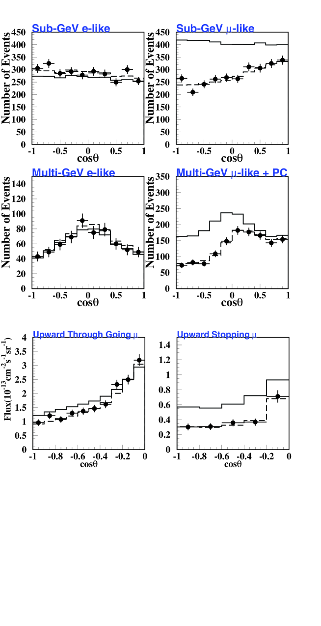
Figure 15: Zenith angle distribution of Super-Kamiokande 1289 day sub-GeV and multi-GeV samples. Solid and dashed lines correspond to MC with no oscillation and MC with best fit oscillation parameters, respectively [46].

It appears natural to interpret the observed $\nu_{\mu}$ deficit again in terms of neutrino oscillations. This hypothesis is further strengthened by the analysis of the zenith angle dependence shown in fig. 15. No deficit is seen for electron-neutrinos. On the contrary, for muon-neutrinos the deficit is the larger, the larger the zenith angle, i.e. the larger the distance between detector and production point in the earth’s atmosphere. For upward going neutrinos the oscillation length is about 13.000 km.

For neutrinos with energies ${\cal O}$(GeV) one has a sensitivity for mass splittings down to $\Delta m^{2}\sim 10^{-4}$ eV². A two-flavour analysis $\nu_{\mu}\rightarrow\nu_{a}$ yields for the allowed parameter range at 90% CL,

$$\sin^{2}{2\Theta_{0}}>0.88\;,\quad 1.6\times 10^{-3}<\Delta m^{2}<4\times 10^{-3}\;.$$ (127)

For oscillations into sterile neutrinos, $\nu_{\mu}\rightarrow\nu_{s}$, earth matter effects become important. A detailed analysis shows that this case is disfavoured.

Important information on neutrino mixing is also obtained from reactor experiments. Failure to observe $\overline{\nu}_{e}\rightarrow\overline{\nu}_{x}$ oscillations gives the bound [47], for $\Delta m^{2}_{31}\simeq 3\times 10^{-3}$ eV²,

$$\sin^{2}{2\Theta_{0}}<0.12\;.$$ (128)

For three active neutrinos, this suggests a small mixing between the first and the third generation.

4.3.3 Future prospects

In the coming years we can look forward to important results from several experiments. Mini-BooNE at Fermilab will verify or falsify the LSND signal for oscillations. The long-baseline experiments K2K and MINOS will be able to verify $\nu_{\mu}-\nu_{\alpha}$ oscillations and to determine the mass difference $\Delta m^{2}_{23}$ more precisely. Correspondingly, OPERA and ICARUS at Gran Sasso, using the muon-neutrino beam from CERN, will look for $\tau$ appearance, verifying unequivocally $\nu_{\mu}-\nu_{\tau}$ oscillations. The first oscillation dip could be studied by MONOLITH. The ${}^{7}Be$ line of solar neutrinos will be studied by Borexino.

KamLAND is the first terrestrial experiment sensitive to the solar neutrino signal (fig. 16). Using reactor neutrinos over a baseline of about 175 km it could verify the LMA solution of the solar neutrino problem. This would be of crucial importance for the prospects of observing CP violation in neutrino oscillations. This may then be possible in neutrino superbeam experiments (JHF in Japan, SPL at CERN) or, eventually, at a neutrino factory.

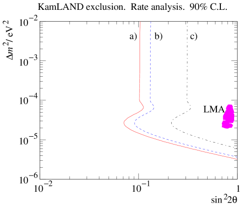
Figure 16: Sensitivity of the KamLAND neutrino oscillation experiment. The curves represent 90% CL limits which can be reached in 3 years of running. The cases a) - c) correspond to different assumptions about the background [48].

The result of neutrino oscillation experiments will be the determination of neutrino mass differences and the leptonic mixing matrix. At present, a three-flavour analysis assuming the LMA solution leads to the following result [49],

$$U=\left(\begin{array}[]{ccc}0.74-0.90&0.45-0.65&<0.16\\ 0.22-0.61&0.46-0.77&0.57-0.71\\ 0.14-0.55&0.36-0.68&0.71-0.82\end{array}\right)\;.$$ (129)

The emerging structure is very remarkable and completely different from the CKM matrix of quark mixing. Whereas $V_{CKM}$ is strongly hierarchical, all elements of the leptonic mixing matrix $U$ are of the same order, except $U_{e3}$, for which only an upper bound exists. This has important implications for the structure of fermion masses in unified theories.

5 Neutrino Masses in GUTs

Neutrino masses and their relation to quark and charged lepton masses play an important role in grand unified theories. According to the seesaw mechanism the smallness of the light neutrino masses is explained by the largeness of the heavy Majorana neutrino masses, which extend up to the mass scale of unification. Hence, the present experimental evidence for neutrino masses and mixings probes for the first time the physics of unification. Reviews and extensive references are given in ref. [50], a special approach is described in ref. [51].

5.1 Elements of grand unified theories

Let us first consider the basic ingredients of GUTs, starting from the symmetries of the standard model where neutrinos are massless. As a consequence, four ‘charges’ are classically conserved, three lepton numbers and baryon number,

$$L_{e}\;,\quad L_{\mu}\;,\quad L_{\tau}\;,\quad B\;.$$ (130)

Figure 17: ABJ-anomaly of the $B-L$ current.

The Adler-Bell-Jackiw anomaly (fig. 17), a quantum effect, reduces the four conserved charges to three [52], which may be chosen as,

$$L_{e}-L_{\mu}\;,\quad L_{\mu}-L_{\tau}\;,\quad B-L\;,$$ (131)

where $L=L_{e}+L_{\mu}+L_{\tau}$ is the total lepton number. One may wonder whether these charges correspond to fundamental global symmetries, or whether they are just accidental symmetries of the low-energy effective theory, similar to weak isospin which is an approximate symmetry of weak interactions at energies much below the W-boson mass.

Neutrino masses and mixings break the first two of these symmetries, $L_{e}-L_{\mu}$ and $L_{\mu}-L_{\tau}$, but presently we do not know whether $B-L$ is a fundamental symmetry or not. $B-L$ is conserved if neutrinos have only Dirac masses and the Majorana masses of the right-handed neutrinos vanish,

$$m_{D}=h_{\nu}\langle H_{1}\rangle\;,\quad M=0\;.$$ (132)

Note, that this requires tiny Yukawa couplings, e.g. $h_{\nu 22}\sim 10^{-14}$ for $m_{\nu 2}\sim 5\times 10^{-3}$ eV. This possibility can presently not be excluded although it might appear unnatural. Alternatively, $B-L$ may be broken at some intermediate mass scale or at the GUT scale $\Lambda\sim 10^{16}$ GeV, where the gauge couplings unify in the supersymmetric standard model (fig. 18). This is indeed suggested by the smallness of the observed neutrino masses in connection with the seesaw mechanism. With $h_{\nu 33}={\cal O}(1)$ one obtains for the mass of the heaviest Majorana neutrino from eq. (52),

$$M_{3}\sim{\langle H_{1}\rangle^{2}\over m_{\nu_{3}}}\sim 10^{15}\ \mbox{GeV}\sim\Lambda_{GUT}\;.$$ (133)

Figure 18: Unification of gauge couplings in the supersymmetric standard model.

The unification of gauge couplings suggests that the standard model gauge group is part of a larger simple group,

$$G_{SM}=U(1)\times SU(2)\times SU(3)\subset SU(5)\subset\ldots\;.$$ (134)

The simplest GUT is based on the gauge group SU(5) [53]. Here quarks and leptons are grouped into the multiplets,

$${\bf 10}=(q_{L},u_{R}^{c},e_{R}^{c})\;,\quad{\bf 5^{*}}=(d_{R}^{c},l_{L})\;,\quad{\bf 1}=\nu_{R}\;.$$ (135)

Note that, unlike gauge fields, quarks and leptons are not unified in a single irreducible representation. In particular, the right-handed neutrinos are gauge singlets and can therefore have Majorana masses not generated by spontaneous symmetry breaking. In addition one has three Yukawa interactions, which couple the fermions to the Higgs fields $H_{1}({\bf 5})$ and $H_{2}({\bf 5^{*}})$,

$${\cal L}=h_{uij}{\bf 10}_{i}{\bf 10}_{j}H_{1}({\bf 5})+h_{dij}{\bf 5^{*}}_{i}{\bf 10}_{j}H_{2}({\bf 5^{*}})+h_{\nu ij}{\bf 5^{*}}_{i}{\bf 1}_{j}H_{1}({\bf 5})+M_{ij}{\bf 1}_{i}{\bf 1}_{j}\;.$$ (136)

The mass matrices of up-quarks, down-quarks, charged leptons and the Dirac neutrino mass matrix are given by $m_{u}=h_{u}v_{1}$, $m_{d}=h_{d}v_{2}=m_{e}$ and $m_{D}=h_{\nu}v_{1}$, respectively, with $v_{1}=\langle H_{1}\rangle$ and $v_{2}=\langle H_{2}\rangle$. The SU(5) mass relation $m_{d}=m_{e}$ is successful for the third generation but requires substantial corrections for the second and first generations. The Majorana masses $M$ are independent of the Higgs mechanism and can therefore be much larger than the electroweak scale $v$.

Once right-handed neutrinos are introduced, the $B-L$ charges of each generation add up to zero. Hence, there are no mixed $B-L$ $-$ gravitational anomalies (fig. 19), and the U(1)_B-L symmetry can be embedded together with SU(5) into a larger GUT group.

Figure 19: Mixed $B-L$ $-$ gravitational anomaly.

In this way one arrives at the gauge group SO(10) [54]. All quarks and leptons of one generation are now contained in a single multiplet,

$${\bf 16}=(q_{L},u_{R}^{c},e_{R}^{c},d_{R}^{c},l_{L},\nu_{R})\;.$$ (137)

Quark and lepton mass matrices are obtained from the couplings of the fermion multiplets ${\bf 16}_{i}$ to the Higgs multiplets $H_{1}({\bf 10})$, $H_{2}({\bf 10})$ and $\Phi({\bf 126})$,

$${\cal L}=h_{uij}{\bf 16}_{i}{\bf 16}_{j}H_{1}({\bf 10})+h_{dij}{\bf 16}_{i}{\bf 16}_{j}H_{2}({\bf 10})+h_{Nij}{\bf 16}_{i}{\bf 16}_{j}\Phi({\bf 126})\;.$$ (138)

Here we have assumed that the two Higgs doublets of the standard model are contained in the two 10-plets $H_{1}$ and $H_{2}$, respectively. This yields the quark mass matrices $m_{u}=h_{u}v_{1}$, $m_{d}=h_{d}v_{2}$, with $v_{1}=\langle H_{1}\rangle$ and $v_{2}=\langle H_{2}\rangle$, and the lepton mass matrices

$$m_{D}=m_{u}\;,\quad m_{e}=m_{d}\;.$$ (139)

Contrary to SU(5) GUTs, the Dirac neutrino and the up-quark mass matrices are now related. Note, that all matrices are symmetric. The Majorana mass matrix $M=h_{N}\left\langle\Phi\right\rangle$, which is also generated by spontaneous symmetry, is a priori independent of $m_{u}$ and $m_{d}$.

In the literature also GUT groups larger than SO(10) have been studied. Particularly interesting is the sequence of exceptional groups which terminates at rank 8,

$$E_{4}=SU(5)\subset E_{5}=SO(10)\subset E_{6}\subset E_{7}\subset E_{8}\;.$$ (140)

The last two groups can also unify different generations and thereby restrict the Yukawa matrices. They arise naturally in higher dimensional supergravity theories and in string theories.

What are the GUT predictions for neutrino masses and mixings? As emphasized at the end of section 4.3.3, the emerging structure of the leptonic mixing matrix appears to be remarkably simple,

$$U=\left(\begin{array}[]{ccc}\ast&\ast&\diamond\\ \ast&\ast&\ast\\ \ast&\ast&\ast\end{array}\right)\;,$$ (141)

where the ‘$\ast$’ denotes matrix elements whose value is consistent with the range $0.5\ldots 0.8$, whereas for the matrix element ‘$\diamond$’ only an upper bound exits, $|U_{e3}|<0.16$.

There are several interesting ‘Ansätze’ to explain this pattern, such as ‘bi-maximal’ mixing ($\Theta_{12}=\Theta_{23}=45^{o}$, $\Theta_{13}=0$),

$$U=\left(\begin{array}[]{ccc}{1\over\sqrt{2}}&-{1\over\sqrt{2}}&0\\ {1\over 2}&{1\over 2}&-{1\over\sqrt{2}}\\ {1\over 2}&{1\over 2}&{1\over\sqrt{2}}\end{array}\right)\;,$$ (142)

or ‘democratic mixing’ where in the weak eigenstate basis all elements are equal to 1, which leads to the mixing matrix,

$$U=\left(\begin{array}[]{ccc}{1\over\sqrt{2}}&-{1\over\sqrt{2}}&0\\ {1\over\sqrt{6}}&{1\over\sqrt{6}}&-{2\over\sqrt{6}}\\ {1\over\sqrt{3}}&{1\over\sqrt{3}}&{1\over\sqrt{3}}\end{array}\right)\;.$$ (143)

Further, one can also construct ‘tri-bimaximal’ mixing [55]. All these patterns are interesting. In general, however, they lack an underlying symmetry. In the following we shall restrict our discussion to constraints on neutrino masses which arise for the simplest GUT groups, SU(5) and SO(10).

An important consequence of neutrino mixing are flavour changing processes and electric dipole moments of charged leptons [56]. In particular supersymmetric theories predict effects large enough to be discovered in the near future, even before the start of LHC.

5.2 Models with SU(5)

An attractive framework to explain the observed mass hierarchies of quarks and charged leptons is the Froggatt-Nielsen mechanism [57] based on a spontaneously broken U(1)_F generation symmetry. The Yukawa couplings are assumed to arise from non-renormalizable interactions after a gauge singlet field $\Phi$ acquires a vacuum expectation value,

$$h_{ij}=g_{ij}\left({\left\langle\Phi\right\rangle\over\Lambda}\right)^{Q_{i}+Q_{j}}\;.$$ (144)

Here $g_{ij}$ are couplings ${\cal O}(1)$, and $Q_{i}$ are the U(1)_F charges of the various fermions, with $Q_{\Phi}=-1$. The interaction scale $\Lambda$ is usually chosen to be very large, $\Lambda>\Lambda_{GUT}$.

$\psi_{i}$	$\bf 10_{3}$	$\bf 10_{2}$	$\bf 10_{1}$	$\bf 5^{*}_{3}$	$\bf 5^{*}_{2}$	$\bf 5^{*}_{1}$	$\bf 1_{3}$	$\bf 1_{2}$	$\bf 1_{1}$
$Q_{i}$	0	1	2	$a$	$a$	$a+1$	b	$c$	$d$

Table 2: Lopsided U(1)_F charges of SU(5) multiplets.

The symmetry group SU(5)$\times$U(1)_F has been considered by a number of authors. Particularly interesting is the case with a ‘lopsided’ family structure where the chiral U(1)_F charges are different for the $\bf 5^{*}$-plets and the $\bf 10$-plets of the same family [58]-[61]. Note, that such lopsided charge assignments are not consistent with the embedding into a higher-dimensional gauge group, like SO(10)$\times$U(1)_F or E${}_{6}\times$U(1)_F. An example of phenomenologically allowed lopsided charges $Q_{i}$ is given in table 2.

The charge assignements determine the structure of the Yukawa matrices, e.g.,

$$h_{e},h_{\nu}\ \sim\ \left(\begin{array}[]{ccc}\epsilon^{3}&\epsilon^{2}&\epsilon^{2}\\ \epsilon^{2}&\;\epsilon&\epsilon\\ \epsilon&1&1\end{array}\right)\;,$$ (145)

where the parameter $\epsilon=\left\langle\Phi\right\rangle/\Lambda$ controls the flavour mixing, and coefficients ${\cal O}(1)$ are unknown. The corresponding mass hierarchies for up-quarks, down-quarks and charged leptons are,

$$\qquad\quad m_{t}:m_{c}:m_{u} \simeq 1:\epsilon^{2}:\epsilon^{4}\;,$$ (146)

$$m_{b}:m_{s}:m_{d} = m_{\tau}:m_{\mu}:m_{e}\simeq 1:\epsilon:\epsilon^{3}\;.$$ (147)

The differences between the observed down-quark mass hierarchy and the charged lepton mass hierarchy can be accounted for by introducing additional Higgs fields [62]. From a fit to the running quark and lepton masses at the GUT scale the flavour mixing parameter is determined as $\epsilon\simeq 0.06$.

The light neutrino mass matrix is obtained from the seesaw formula,

$$m_{\nu}=-m_{D}{1\over M}m_{D}^{T}\ \sim\ \epsilon^{2a}\left(\begin{array}[]{ccc}\epsilon^{2}&\epsilon&\epsilon\\ \epsilon&\;1&1\\ \epsilon&1&1\end{array}\right)\;.$$ (148)

Note, that the structure of this matrix is determined by the U(1)_F charges of the $\bf 5^{*}$-plets only. It is independent of the U(1)_F charges of the right-handed neutrinos.

Since all elements of the 2-3 submatrix of (148) are ${\cal O}(1)$, one naturally obtains a large $\nu_{\mu}-\nu_{\tau}$ mixing angle $\Theta_{23}$ [58, 59]. At first sight one may expect $\Theta_{12}={\cal O}(\epsilon)$, which would correspond to the SMA solution of the MSW effect. However, one can also have a large mixing angle $\Theta_{12}$ if the determinant of the 2-3 submatrix of $m_{\nu}$ is ${\cal O}(\epsilon)$ [63]. Choosing the coefficients ${\cal O}(1)$ randomly, in the spirit of ‘flavour anarchy’ [39], the SMA and the LMA solutions are about equally probable for $\epsilon\simeq 0.1$ [64]. The corresponding neutrino masses are consistent with $m_{2}\sim 5\times 10^{-3}$ eV and $m_{3}\sim 5\times 10^{-2}$ eV. We conclude that the neutrino mass matrix (148) naturally yields a large angle $\Theta_{23}$, with $\Theta_{12}$ being either large or small. In order to have maximal mixings the coefficients ${\cal O}(1)$ have to obey special relations.

5.3 Models with SO(10)

Neutrino masses in SO(10) GUTs have been extensively discussed in the literature [65]. Since all quarks and leptons are unified in a single multiplet these models often have difficulties to reconcile the large neutrino mixings with the small quark mixings. In the following we shall illustrate this problem by means of an example [66] which only makes use of the seesaw relation, the SO(10) relation between the up-quark and Dirac neutrino mass matrices,

$$m_{u}=m_{D}\;,$$ (149)

and the empirically known properties of the up-quark mass matrix.

With $m_{D}=m_{u}$ the seesaw mass relation becomes

$$m_{\nu}\simeq-m_{u}{1\over M}m_{u}^{T}\;.$$ (150)

The large neutrino mixings now appear very puzzling, since the quark mass matrices are hierarchical and the quark mixings are small. It turns out, however, that because of the known properties of the up-quark mass matrix this puzzle can be resolved provided the heavy neutrino masses also obey a specific hierarchy. This then leads to predictions for a number of observables in neutrino physics including the cosmological baryon asymmetry.

From the phenomenology of weak decays we know that the quark matrices have approximately the form [67],

$$m_{u,d}\propto\left(\begin{array}[]{ccc}0&\epsilon^{3}e^{i\phi}&0\\ \epsilon^{3}e^{i\phi}&\;\rho\epsilon^{2}&\eta\epsilon^{2}\\ 0&\eta\epsilon^{2}&e^{i\psi}\end{array}\right)\;.$$ (151)

Here $\epsilon\ll 1$ is the parameter which determines the flavour mixing, and $\rho=|\rho|e^{i\alpha}$, $\eta=|\eta|e^{i\beta}$ are complex parameters ${\cal O}(1)$. We have chosen a ‘hierarchical’ basis, where off-diagonal matrix elements are small compared to the product of the corresponding eigenvalues, $|m_{ij}|^{2}\leq{\cal O}(|m_{i}m_{j}|)$. In contrast to the usual assumption of hermitian mass matrices, SO(10) invariance dictates the matrices to be symmetric. All parameters may take different values for up$-$ and down$-$quarks. Typical choices for $\epsilon$ are $\epsilon_{u}\simeq 0.07$, $\epsilon_{d}\simeq 0.2$. The agreement with data can be improved by adding in the 1-3 element a term ${\cal O}(\epsilon^{4})$ which, however, is not important for the following analysis. In case of a 1-3 element ${\cal O}(\epsilon^{3})$, one can have a SU(3) generation symmetry leading to different results [68]. Data also fix one product of phases to be ‘maximal’, i.e. $\Delta=\phi_{u}-\alpha_{u}-\phi_{d}+\alpha_{d}\simeq\pi/2$.

We do not know the structure of the Majorana mass matrix $M=h_{N}\left\langle\Phi\right\rangle$. However, in models with family symmetries it should be similar to the quark mass matrices, i.e. the structure should be independent of the Higgs field. In this case, one expects

$$M=\left(\begin{array}[]{ccc}0&M_{12}&0\\ M_{12}&M_{22}&M_{23}\\ 0&M_{23}&M_{33}\end{array}\right)\;,$$ (152)

with $M_{12}\ll M_{22}\sim M_{23}\ll M_{33}$. The symmetric mass matrix $M$ is diagonalized by a unitary matrix,

$$U^{(N)\dagger}MU^{(N)*}=\left(\begin{array}[]{ccc}M_{1}&0&0\\ 0&M_{2}&0\\ 0&0&M_{3}\end{array}\right).$$ (153)

Using the seesaw formula one can now evaluate the light neutrino mass matrix. Since the choice of the Majorana matrix $M$ fixes a basis for the right-handed neutrinos the allowed phase redefinitions of the Dirac mass matrix $m_{D}$ are restricted. In eq. (151) the phases of all matrix elements have therefore been kept.

The $\nu_{\mu}$-$\nu_{\tau}$ mixing angle is known to be large. This leads us to require $m_{\nu_{i,j}}={\cal O}(1)$ for $i,j=2,3$. It is remarkable that this determines the hierarchy of the heavy Majorana mass matrix to be

$$M_{12}:M_{22}:M_{33}=\epsilon^{5}:\epsilon^{4}:1\;.$$ (154)

With $M_{33}\simeq M_{3}$, $M_{22}=\sigma\epsilon^{4}M_{3}$, $M_{23}=\zeta\epsilon^{4}M_{3}\sim M_{22}$ and $M_{12}=\epsilon^{5}M_{3}$, one obtains for masses and mixings to order ${\cal O}(\epsilon^{4})$,

$$M_{1}\simeq-{\epsilon^{6}\over\sigma}M_{3}\;,\quad M_{2}\simeq\sigma\epsilon^{4}M_{3}\;,$$ (155)

with $U^{(N)}_{12}=-U^{(N)}_{21}=\epsilon/\sigma$, $U^{(N)}_{23}={\cal O}(\epsilon^{4})$ and $U^{(N)}_{13}=0$. Note, that $\sigma$ can always be chosen real. This yields for the light neutrino mass matrix

$$m_{\nu}=-\left(\begin{array}[]{ccc}0&\epsilon e^{2i\phi}&0\\ \epsilon e^{2i\phi}&-\sigma e^{2i\phi}+2\rho e^{i\phi}&\eta e^{i\phi}\\ 0&\eta e^{i\phi}&\;e^{2i\psi}\end{array}\right)\ {v_{1}^{2}\over M_{3}}\;.$$ (156)

The complex parameter $\zeta$ does not enter because of the hierarchy. The matrix (156) has the same structure as the mass matrix (148) in the SU(5)$\times$U(1)_F model, except for additional texture zeroes. Since, as required, all elements of the 2-3 submatrix are ${\cal O}(1)$, the mixing angle $\Theta_{23}$ is naturally large. A large mixing angle $\Theta_{12}$ can again occur in case of a small determinant of the 2-3 submatrix. Such a condition can be fullfilled without fine tuning for $\sigma,\rho,\eta={\cal O}(1)$.

The mass matrix $m_{\nu}$ is again diagonalized by a unitary matrix, $U^{(\nu)\dagger}m_{\nu}U^{(\nu)*}=\mbox{diag}(m_{1},m_{2},m_{3})$. A straightforward calculation yields ($s_{ij}=\sin{\Theta_{ij}}$, $c_{ij}=\cos{\Theta_{ij}}$, $\xi=\epsilon/(1+|\eta|^{2})$),

$$U^{(\nu)}=\left(\begin{array}[]{ccc}c_{12}e^{i(\phi-\beta+\psi-\gamma)}&s_{12}e^{i(\phi-\beta+\psi-\gamma)}&\xi s_{23}e^{i(\phi-\beta+\psi)}\\ -c_{23}s_{12}e^{i(\phi+\beta-\psi+\gamma)}&c_{23}c_{12}e^{i(\phi+\beta-\psi+\gamma)}&s_{23}e^{i(\phi+\beta-\psi)}\\ s_{23}s_{12}e^{i(\gamma+\psi)}&-s_{23}c_{12}e^{i(\gamma+\psi)}&c_{23}e^{i\psi}\end{array}\right)\;,$$ (157)

with the mixing angles,

$$\tan{2\Theta_{23}}\simeq{2|\eta|\over 1-|\eta|^{2}}\;,\quad\tan{2\Theta_{12}}\simeq 2\sqrt{1+|\eta|^{2}}{\epsilon\over\delta}\;.$$ (158)

Note, that the 1-3 element of the mixing matrix is small, $U^{(\nu)}_{13}={\cal O}(\epsilon)$. The masses of the light neutrinos are

$$m_{1}\simeq-\tan^{2}{\Theta_{12}}\ m_{2}\;,\quad m_{2}\simeq{\epsilon\over(1+|\eta|^{2})^{3/2}}\cot{\Theta_{12}}\ m_{3}\;,\quad m_{3}\simeq(1+|\eta|^{2})\ {v_{1}^{2}\over M_{3}}\;.$$ (159)

This corresponds to the weak hierarchy,

$$m_{1}:m_{2}:m_{3}=\epsilon:\epsilon:1\;,$$ (160)

with $m_{2}^{2}\sim m_{1}^{2}\sim\Delta m_{21}^{2}=m_{2}^{2}-m_{1}^{2}\sim\epsilon^{2}$. Since $\epsilon\sim 0.1$, this pattern is consistent with the LMA solution of the solar neutrino problem, but not with the LOW solution.

The large $\nu_{\mu}$-$\nu_{\tau}$ mixing is related to the very large mass hierarchy (155) of the heavy Majorana neutrinos. The large $\nu_{e}$-$\nu_{\mu}$ mixing follows from the particular values of parameters ${\cal O}(1)$. Hence, one expects two large mixing angles, but single maximal or bi-maximal mixing would require fine tuning. On the other hand, one definite prediction is the occurence of exactly one small matrix element, $U^{(\nu)}_{13}={\cal O}(\epsilon)$. Note, that the obtained pattern of neutrino mixings is independent of the off-diagonal elements of the mass matrix $M$. For instance, replacing the texture (152) by a diagonal matrix, $M=\mbox{diag}(M_{1},M_{2},M_{3})$, leads to the same pattern of neutrino mixings.

In order to calculate various observables in neutrino physics we need the leptonic mixing matrix

$$U=U^{(e)\dagger}U^{(\nu)}\;,$$ (161)

where $U^{(e)}$ is the charged lepton mixing matrix. In our framework we expect $U^{(e)}\simeq V^{(d)}$, and also $V=V^{(u)\dagger}V^{(d)}\simeq V^{(d)}$ for the CKM matrix since $\epsilon_{u}<\epsilon_{d}$. This yields for the leptonic mixing matrix

$$U\simeq V^{\dagger}U^{(\nu)}\;.$$ (162)

To leading order in the Cabibbo angle $\lambda\simeq 0.2$ we only need the off-diagonal elements $V^{(d)}_{12}=\overline{\lambda}=-V^{(d)*}_{21}$. Since the matrix $m_{d}$ is complex, the Cabibbo angle is modified by phases, $\overline{\lambda}=\lambda\exp{\{i(\phi_{d}-\alpha_{d})\}}$. The resulting leptonic mixing matrix is indeed of the wanted form (141) with all matrix elements ${\cal O}(1)$, except $U_{13}$,

$$U_{13}=\xi s_{23}e^{i(\phi-\beta+\psi)}-\overline{\lambda}s_{23}e^{i(\phi+\beta-\psi)}={\cal O}(\lambda,\epsilon)\sim 0.1\;,$$ (163)

which is close to the experimental limit.

Let us now consider the CP violation in neutrino oscillations. Observable effects are controlled by the Jarlskog parameter (cf. (95)) for which one finds

$$J_{l}\simeq{\lambda\over 4\sqrt{2}}\sin{\delta}\;,$$ (164)

where $\delta$ is some function of the unknown parameters ${\cal O}(1)$. Due to the large neutrino mixing angles, $J_{l}$ can be much bigger than the Jarlskog parameter in the quark sector, $J_{q}={\cal O}(\lambda^{6})\sim 10^{-5}$.

According to the seesaw mechanism neutrinos are Majorana fermions. This can be directly tested in neutrinoless double $\beta$-decay. The decay amplitude is proportional to the complex mass

$$\left\langle m\right\rangle=\sum_{i}U_{ei}^{2}m_{i}=-{1\over 1+|\eta|^{2}}\left(\lambda^{2}|\eta|^{2}e^{2i(\phi_{d}-\alpha_{d}+\beta+\phi-\psi)}-2\lambda\epsilon e^{i(\phi_{d}-\alpha_{d}+2\phi)}\right)m_{3}\;.$$ (165)

With $m_{3}\simeq\sqrt{\Delta m^{2}_{atm}}\simeq 5\times 10^{-2}$ eV this yields $\left\langle m\right\rangle\sim 10^{-3}$ eV, more than two orders of magnitude below the present experimental upper bound [14].

6 Leptogenesis

One of the main successes of the standard early-universe cosmology is the prediction of the abundances of the light elements, D, ³He, ⁴He and ⁷Li. Agreement between theory and observation is obtained for a certain range of the parameter $\eta$, the ratio of baryon density and photon density [10],

$$\eta={n_{B}\over n_{\gamma}}=(1.5-6.3)\times 10^{-10}\;,$$ (166)

where the present number density of photons is $n_{\gamma}\sim 400/{\rm cm}^{3}$. Since no significant amount of antimatter is observed in the universe, the baryon density yields directly the cosmological baryon asymmetry, $Y_{B}=(n_{B}-n_{\bar{B}})/s\simeq\eta/7$, where $s$ is the entropy density.

A matter-antimatter asymmetry can be dynamically generated in an expanding universe if the particle interactions and the cosmological evolution satisfy Sakharov’s conditions [70],

• baryon number violation ,

• $C$ and $C\!P$ violation ,

• deviation from thermal equilibrium .

Although the baryon asymmetry is just a single number, it provides an important relationship between the standard model of cosmology, i.e. the expanding universe with Robertson-Walker metric, and the standard model of particle physics as well as its extensions.

At present there exist a number of viable scenarios for baryogenesis. They can be classified according to the different ways in which Sakharov’s conditions are realized. In grand unified theories $B$ and $L$ are broken by the interactions of gauge bosons and leptoquarks. This is the basis of classical GUT baryogenesis [71]. Analogously, the lepton number violating decays of heavy Majorana neutrinos lead to leptogenesis [72]. In the simplest version of leptogenesis the initial abundance of the heavy neutrinos is generated by thermal processes. Alternatively, heavy neutrinos may be produced in inflaton decays, in the reheating process after inflation, or by brane collisions [73]. The observed magnitude of the baryon asymmetry can be obtained for realistic neutrino masses [74].

The crucial deviation from thermal equilibrium can also be realized in several ways. One possibility is a sufficiently strong first-order electroweak phase transition which makes electroweak baryogenesis possible [75]. For the classical GUT baryogenesis and for leptogenesis the departure from thermal equilibrium is due to the deviation of the number density of the decaying heavy particles from the equilibrium number density. How strong this departure from equilibrium is depends on the lifetime of the decaying heavy particles and the cosmological evolution.

6.1 Baryon and lepton number at high temperatures

The theory of baryogenesis involves non-perturbative aspects of quantum field theory and also non-equilibrium statistical field theory, in particular the theory of phase transitions and kinetic theory.

Figure 20: One of the 12-fermion processes which are in thermal equilibrium in the high-temperature phase of the standard model.

A crucial ingredient is the connection between baryon number and lepton number in the high-temperature, symmetric phase of the standard model. Due to the chiral nature of the weak interactions $B$ and $L$ are not conserved. At zero temperature this has no observable effect due to the smallness of the weak coupling. However, as the temperature approaches the critical temperature $T_{EW}$ of the electroweak transition, $B$- and $L$-violating processes come into thermal equilibrium [76].

The rate of these processes is related to the free energy of sphaleron-type field configurations which carry topological charge. In the standard model they lead to an effective interaction of all left-handed quarks and leptons [52] (cf. fig. 20),

$$O_{B+L}=\prod_{i}\left(q_{Li}q_{Li}q_{Li}l_{Li}\right)\;,$$ (167)

which violates baryon and lepton number by three units,

$$\Delta B=\Delta L=3\;.$$ (168)

The evaluation of the sphaleron rate in the symmetric high-temperature phase is a complicated problem. A clear physical picture has been obtained in Bödeker’s effective theory [77] according to which low-frequency gauge field fluctuations satisfy an equation analogous to electric and magnetic fields in a superconductor,

$${\bf D}\times{\bf B}=\sigma{\bf E}-{\bf\zeta}\;.$$ (169)

Here $\bf\zeta$ represents Gaussian noise, and $\sigma$ is a non-abelian conductivity. The sphaleron rate can then be written as,

$$\Gamma_{SPH}\simeq(14.0\pm 0.3){1\over\sigma}(\alpha_{w}T)^{5}\;.$$ (170)

Lattice simulations [78] have confirmed early estimates that $B$- and $L$-violating processes are in thermal equilibrium for temperatures in the range

$$T_{EW}\sim 100\ \mbox{GeV}<T<T_{SPH}\sim 10^{12}\ \mbox{GeV}\;.$$ (171)

Sphaleron processes have a profound effect on the generation of the cosmological baryon asymmetry, in particular in connection with the dominant lepton number violating interactions between lepton and Higgs fields,

$${\cal L}_{\Delta L=2}={1\over 2}f_{ij}\ l^{T}_{Li}\phi Cl_{Lj}\phi+\mbox{ h.c.}\;.$$ (172)

As discussed in section 3.3, these interactions arise from the exchange of heavy Majorana neutrinos, with $\phi=H_{1}$ and $f_{ij}=-(h_{\nu}M^{-1}h^{T}_{\nu})_{ij}$. In the Higgs phase of the standard model, where the Higgs field acquires a vacuum expectation value, the interaction (172) leads to Majorana masses for the light neutrinos $\nu_{e}$, $\nu_{\mu}$ and $\nu_{\tau}$.

One may be tempted to conclude from eq. (168) that any $B+L$ asymmetry generated before the electroweak phase transition, i.e. at temperatures $T>T_{EW}$, will be washed out. However, since only left-handed fields couple to sphalerons, a non-zero value of $B+L$ can persist in the high-temperature, symmetric phase in case of a non-vanishing $B-L$ asymmetry. An analysis of the chemical potentials of all particle species in the high-temperature phase yields a relation between the baryon asymmetry $Y_{B}=(n_{B}-n_{\bar{B}})/s$ and the corresponding $B-L$ and $L$ asymmetries $Y_{B-L}$ and $Y_{L}$, respectively,

$$Y_{B}\ =\ a\ Y_{B-L}\ =\ {a\over a-1}\ Y_{L}\;.$$ (173)

The number $a$ depends on the other processes which are in thermal equilibrium. If these are all standard model interactions one has $a=8/23$ in the case of two Higgs doublets [79].

From eq. (173) one concludes that the cosmological baryon asymmetry requires also a lepton asymmetry, and therefore lepton number violation. This leads to an intriguing interplay between Majorana neutrinos masses, which are generated by the lepton-Higgs interactions (172), and the baryon asymmetry: lepton number violating interactions are needed in order to generate a baryon asymmetry; however, they have to be sufficiently weak, so that they fall out of thermal equilibrium at the right time and a generated asymmetry can survive until today.

6.2 Thermal leptogenesis

Figure 21: Tree level and one-loop diagrams contributing to heavy neutrino decays.

Let us now consider the simplest possibility for a departure from thermal equilibrium, the decay of heavy, weakly interacting particles in a thermal bath. We choose the heavy particle to be the lightest of the heavy Majorana neutrinos, $N_{1}\equiv N=N^{c}$, which can decay into a lepton Higgs pair $l\phi$ and also into the $C\!P$ conjugate state $\bar{l}\bar{\phi}$,

$$N\rightarrow l\;\phi\;,\quad N\rightarrow\bar{l}\;\bar{\phi}\;.$$ (174)

In the case of $C\!P$ violating couplings a lepton asymmetry can be generated in the decays of the heavy neutrinos $N$,

$$\Gamma(N\rightarrow l\phi)={1\over 2}(1+\varepsilon_{1})\Gamma\;,\quad\Gamma(N\rightarrow\bar{l}\bar{\phi})={1\over 2}(1-\varepsilon_{1})\Gamma\;,$$ (175)

where $\Gamma$ is the total decay width and $\varepsilon_{1}\ll 1$ measures the amount of $C\!P$ violation.

Figure 22: $\Delta L=1$ processes: decays and inverse decays of a heavy Majorana neutrino.

The $C\!P$ asymmetry $\varepsilon_{1}$ arises from one-loop vertex and self-energy corrections (fig. 21) [80, 81, 82]. It can be expressed in a compact form, which in the mass eigenstate basis of the heavy neutrinos reads,

$$\varepsilon_{1}\simeq{3\over 16\pi}\mbox{sign}(M_{1}){\mbox{Im}\left(m_{D}^{\dagger}m_{\nu}m_{D}^{*}\right)_{11}\over v_{1}^{2}\widetilde{m}_{1}}\;.$$ (176)

Here, in addition to the mass matrices $m_{D}$ and $m_{\nu}$, an effective neutrino mass,

$$\widetilde{m}_{1}={\left(m_{D}^{\dagger}m_{D}\right)_{11}\over|M_{1}|}\;,$$ (177)

appears, which is a sensitive parameter for successful leptogenesis [83]. Note, that the maximal $C\!P$ asymmetry is related to the mass $M_{1}$ of the heavy Majorana neutrino $N_{1}$ [84]. In the case of mass differences of order the decay widths, $|M_{i}-M_{1}|={\cal O}(\Gamma_{i},\Gamma_{1})$, $i\neq 1$, the $C\!P$ asymmetry is enhanced [85]. Contrary to the case considered here, decays of $N_{2}$ or $N_{3}$ may be the origin of the baryon asymmetry [86], if washout effects are sufficiently small.

The generation of a baryon asymmetry is an out-of-equilibrium process which is generally treated by means of Boltzmann equations [71]. The main processes in the thermal bath are the decays and the inverse decays of the heavy neutrinos (fig. 22), and the lepton number conserving ($\Delta L=0$) and violating ($\Delta L=2$) processes (fig. 23). In addition there are other processes, in particular those involving the t-quark, which are important in a quantitative analysis [87, 83].

Figure 23: $\Delta L=0$ and $\Delta L=2$ lepton Higgs processes.

A typical solution of the Boltzmann equations is shown in fig. 24. Here the ratios of number densities and entropy density,

$$Y_{X}={n_{X}\over s}\;,$$ (178)

are plotted, which remain constant for an expanding universe in thermal equilibrium. A heavy neutrino, which is weakly coupled to the thermal bath, falls out of thermal equilibrium at temperatures $T\sim M$, since its decay is too slow to follow the rapidly decreasing equilibrium distribution $f_{N}\sim\exp(-\beta M)$. This leads to an excess of the number density, $n_{N}>n_{N}^{eq}$. $C\!P$ violating partial decay widths then yield a lepton asymmetry which, by means of sphaleron processes, is partially transformed into a baryon asymmetry.

The $C\!P$ asymmetry $\varepsilon_{1}$ (176) leads to a lepton asymmetry in the course of the cosmological evolution, which is then partially transformed into a baryon asymmetry [72] by sphaleron processes,

$$Y_{B}\ =\ {n_{L}-n_{\overline{L}}\over s}\ =\ c_{S}\kappa\ {\varepsilon_{1}\over g_{*}}\;,$$ (179)

where $c_{S}=-8/15$ is the sphaleron conversion factor in the case of two Higgs doublets. In order to determine the washout factor $\kappa<1$ one has to solve the Boltzmann equations. Compared to other scenarios of baryogenesis this leptogenesis mechanism has the advantage that, at least in principle, the resulting baryon asymmetry is entirely determined by neutrino properties.

Figure 24: Time evolution of the number density to entropy density ratio. At $T\sim M$ the system gets out of equilibrium and an asymmetry is produced.

We are now ready to determine the baryon asymmetries predicted by the models of neutrino masses discussed in section 5. Since for the Yukawa couplings only the powers in $\epsilon$ are known, we will also obtain the $C\!P$ asymmetry and the corresponding baryon asymmetry to leading order in $\epsilon$, i.e. up to unknown factors ${\cal O}(1)$.

Consider first the model with symmetry group SU(5)$\times$U(1)_F (cf. section 5.2). One easily obtains from eqs. (145), (176) and table 2,

$$\varepsilon_{1}\ \sim\ {3\over 16\pi}\ \epsilon^{4}\;.$$ (180)

With $\epsilon^{2}\sim 1/300$ and $g_{*}\sim 100$ this yields the baryon asymmetry,

$$Y_{B}\sim\kappa\ 10^{-8}\;.$$ (181)

For $\kappa\sim 0.1\ldots 0.01$ this is indeed the correct order of magnitude. The baryogenesis temperature is given by the mass of the lightest of the heavy Majorana neutrinos,

$$T_{B}\sim M_{1}\sim\epsilon^{4}M_{3}\sim 10^{10}\ \mbox{GeV}\;.$$ (182)

This is essentially the model studied in ref. [88], where the $C\!P$ asymmetry is determined by the mass hierarchy of light and heavy Majorana neutrinos. It is remarkable that the observed baryon asymmety is obtained without any fine tuning of parameters, if $B-L$ is broken at the unification scale $\Lambda_{GUT}$. Note, that the generated baryon asymmetry does not depend on the flavour mixing of the light neutrinos.

Figure 25: Time evolution of the heavy neutrino number density and the lepton asymmetry for the SO(10) model. The upper solid line shows the solution of the Boltzmann equations for the right-handed neutrinos; the equilibrium distribution is represented by the dashed line. The absolute value of the lepton asymmetry $Y_{L}$ is given by the lower solid line, and the hatched area shows the lepton asymmetry corresponding to the observed baryon asymmetry [92].

Figure 26: Same as fig. 25 with initial asymmetry $Y_{L}^{in}\simeq 10^{-2}$ [92].

Qualitatively, the SO(10) model discussed in section 5.3 is very similar. For a class of parameters corresponding to the LMA MSW-solution with $\sigma,\rho,\eta={\cal O}(1)$, one finds for the $C\!P$ asymmetry [66],

$$\varepsilon_{1}\simeq{3\over{16\pi}}\epsilon^{6}{|\eta|^{2}\over\sigma}{(1+|\rho|)^{2}\over|\eta|^{2}+|\rho|^{2}}\sin(\phi_{u}-\alpha_{u})\;.$$ (183)

Note, that except for $\sigma$, the $C\!P$ asymmetry is determined by parameters of the quark mass matrices. Similar results have been obtained in refs. [89, 90] for different models. For a recent analysis within SO(10) models, which favours the Just-So and SMA solar neutrino solutions, see ref. [91].

Numerically, with $\epsilon\sim 0.1$ one finds $\varepsilon_{1}\sim 10^{-7}$ and

$$|M_{1}|\simeq e^{6}{(1+|\eta|^{2})v_{1}^{2}\over\sigma m_{3}}\sim 10^{9}\ \mbox{GeV}\;,$$ (184)

with $\widetilde{m}_{1}\sim(|\eta|^{2}+|\rho|^{2})m_{3}/(\sigma(1+|\eta|^{2}))\sim 10^{-2}$ eV. The baryon asymmetry is then given by

$$Y_{B}\sim-\kappa~{}\mbox{sign}(\sigma)~{}\sin{(\phi_{u}-\alpha_{u})}\times 10^{-9}\;.$$ (185)

The solution of the full Boltzmann equations is shown in fig. 25. The initial condition at a temperature $T\sim 10M_{1}$ is chosen to be a state without heavy neutrinos and with vanishing lepton asymmetry. The Yukawa interactions are sufficient to bring the heavy neutrinos into thermal equilibrium. At temperatures $T\sim M_{1}$ the familiar out-of-equilibrium decays set in, which leads to a non-vanishing baryon asymmetry. The dip in fig. 25 is due to a change of sign in the lepton asymmetry at $T\sim M_{1}$. The final asymmetry is about 1/3 of the observed value, which lies within the present range of theoretical uncertainties.

A very important question for leptogenesis, and baryogenesis in general, is the dependence on initial conditions. As fig. 25 demonstrates, the heavy neutrinos are initially indeed in thermal equilibrium. One may also wonder, how sensitive the final lepton asymmetry is to an initial asymmetry which may have been generated by some other mechanism. The SO(10) model under consideration turns out to be very efficient in establishing a symmetric initial state. This can be seen in fig. 26 where the maximal asymmetry $Y_{L}^{in}\simeq 10^{-2}$ has been assumed as initial condition. Within one order of magnitude in temperature this initial asymmetry is washed out by eight orders of magnitude! Hence, the final baryon asymmetry is a definite prediction of the theory, independent of initial conditions.

In summary, the experimental evidence for small neutrino masses and large neutrino mixings, together with the known small quark mixings, have important implications for the structure of grand unified theories. In SU(5) models this difference between the lepton and quark sectors can be explained by U(1)_F family symmetries. In these models the heavy Majorana neutrino masses are not constrained by low energy physics, i.e. light neutrino masses and mixings. Successful leptogenesis is possible, but it depends on the choice of the heavy Majorana neutrino masses.

In SO(10) models the implications of large neutrino mixings are much more stringent because of the connection between Dirac neutrino and up-quark mass matrices. The requirement of large neutrino mixings then determines the relative magnitude of the heavy Majorana neutrino masses in terms of the known quark mass hierarchy. This leads to predictions for neutrino mixings and masses, $C\!P$ violation in neutrino oscillations and neutrinoless double $\beta$-decay. It is remarkable that the predicted order of magnitude of the baryon asymmetry is also in accord with observation.

I would like to thank the participants of the school for stimulating questions and the organizers for arranging an enjoyable and fruitful meeting at Beatenberg. I have also benefited from discussions with P. Di Bari, M. Plümacher, A. Ringwald, S. Stodolsky and D. Wyler, and I thank S. Wiesenfeldt for providing some of the figures.

References

• [1] N. Bohr, Faraday Lecture, Journal of the Chem. Soc. 1932 (London), p. 349
• [2] W. Pauli, Letter to L. Meitner and H. Geiger, Tübingen, 1930
• [3] E. Majorana, Nuovo Cim. 14 (1937) 171
• [4] E. Fermi, Ricercha Scient. 2 (1933) 12; Z. Physik 88 (1934) 161
• [5] B. Stech, J. H. D. Jensen, Z. Phys. 141 (1955) 175
• [6] E. C. G. Sudarshan, R. E. Marshak, Phys. Rev. 109 (1958) 1860;
R. P. Feynman, M. Gell-Mann, Phys. Rev. 109 (1958) 193
• [7] S. L. Glashow, Nucl. Phys. 22 (1961) 579;
S. Weinberg, Phys. Rev. Lett. 19 (1967) 1264;
A. Salam, in Elementary Particle Theory ed. N Svartholm (Almqvist and Wiksell, Stockholm, 1968) 367
• [8] D. Colladay, V. A. Kostelecky, Phys. Rev. D 58 (1998) 116002;
S. R. Coleman, S.L. Glashow, Phys. Rev. D 59 (1999) 116008
• [9] For reviews and extensive references, see
M. Fukugita, T. Yanagida, Physics of Neutrinos, in Physics and Astrophysics of Neutrinos, eds. M. Fukugita, A. Suzuki (Springer, Tokyo, 1994) 1;
R. N. Mohapatra, P. B. Pal, Massive Neutrinos in Physics and Astrophysics (World Scientific, Singapore, 1998)
• [10] Review of Particle Physics, Eur. Phys. J. C 15 (2000) 1
• [11] DONUT Collaboration, K. Okada, Nucl. Phys. Proc. Suppl. 100 (2001) 256
• [12] Mainz Collaboration, J. Bonn et al., Nucl. Phys. Proc. Suppl. 91 (2001) 273
• [13] Katrin Collaboration, A. Osipowicz et al., hep-ph/0109033
• [14] Heidelberg-Moscow Collaboration, H. V. Klapdor-Kleingrothaus et al., Eur. Phys. J. A12 (2001) 147
• [15] H. V. Klapdor-Kleingrothaus, Nucl. Phys. Proc. Suppl. 100 (2001) 350
• [16] For a recent review and references, see
P. Di Bari, hep-ph/0111056
• [17] AGASA Collaboration, M. Takeda et al., Phys. Rev. Lett. 81 (1998) 1163
• [18] T. Weiler, Phys. Rev. Lett. 49 (1982) 234
• [19] E. Roulet, Phys. Rev. D 47 (1993) 5247
• [20] D. Fargion, B. Mele, A. Salis, Astrophys. J. 517 (1999) 725
• [21] T. J. Weiler, Astropart. Phys. 11 (1999) 303; ibid. 12 (2000) 379 (E)
• [22] Z. Fodor, S. D. Katz, A. Ringwald, hep-ph/0105064
• [23] C. Itzykson, J.-B. Zuber, Quantum Field Theory, McGraw-Hill, New York, 1980
• [24] T. Yanagida, in Workshop on unified Theories, KEK report 79-18 (1979) p. 95;
M. Gell-Mann, P. Ramond, R. Slansky, in Supergravity (North Holland, Amsterdam, 1979) eds. P. van Nieuwenhuizen, D. Freedman, p. 315
• [25] C. Wetterich, Nucl. Phys. B 187 (1981) 343
• [26] R. N. Mohapatra, G. Senjanović, Phys. Rev. D 23 (1981) 165
• [27] For recent work and references, see
M. Hirsch, W. Porod, M. A. Diaz, J. C. Romão, J. W. F. Valle, hep-ph/0202149
• [28] H. Murayama, in ref. [10], p. 360
• [29] S. M. Bilenky, C. Giunti, W. Grimus, Prog. Part. Nucl. Phys. 43 (1999) 1
• [30] E. Kh. Akhmedov, Lectures given at the 1999 Trieste Summer School in Particle Physics, Trieste, Italy, hep-ph/0001264
• [31] B. Kayser, Lectures given at TASI 2000, Boulder, Colarado, hep-ph/0104147
• [32] M. C. Gonzalez-Garcia, Y. Nir, Developments in Neutrino Physics, hep-ph/0202058
• [33] B. Pontecorvo, Zh. Eksp. Teo. Fiz. 33 (1957) 549 [JETP 6 (1958) 429]
• [34] Z. Maki, M. Nakagawa, S. Sakata, Prog. Theor. Phys. 28 (1962) 870
• [35] LSND Collaboration, C. Athanassopoulos et al., Phys. Rev. Lett. 81 (1998) 1774
• [36] L. Stodolsky, Phys. Rev. D 58 (1998) 036006
• [37] A. de Rújula, Neutrinos, Lectures given at the 2000 European School of High Energy Physics, Caramulo, Portugal
• [38] C. Giunti, Quantum Mechanics of Neutrino Oscillations, hep-ph/0105319
• [39] For a recent discussion and references, see
H. Murayama, Theory of Neutrino Masses and Mixings, hep-ph/0201022
• [40] A. de Rújula, M. B. Gavela, P. Hernández, Nucl. Phys. B 547 (1999) 21;
K. Dick, M. Freund, M. Lindner, A. Romanino, Nucl. Phys. B 562 (1999) 29
• [41] S. P. Mikheyev, A. Y. Smirnov, Nuovo Cim. 9C (1986) 17;
L. Wolfenstein, Phys. Rev. D 17 (1978) 2369
• [42] J. N. Bahcall, http://www.sns.ias.edu/ jnb/
• [43] SNO Collaboration, Q. R. Ahmad et al., Phys. Rev. Lett. 87 (2001) 071301
• [44] J. N. Bahcall, M. C. Gonzalez-Garcia, C. Peña-Garay, JHEP 0108 (2001) 014
• [45] G. L. Fogli, E. Lisi, D. Montanino, A. Palazzo, Phys. Rev. D 64 (2001) 093007
• [46] Super-Kamiokande Collaboration, T. Toshito et al., hep-ex/0105023
• [47] CHOOZ, M. Apollonio et al., Phys. Lett. B 466 (1999) 415;
Palo Verde, F. Boehm et al., Nucl. Phys. Proc. Suppl. 91 (2001) 91
• [48] J. Busenitz et al., http://kamland.lbl.gov/
• [49] M. Fukugita, M. Tanimoto, Phys. Lett. B 515 (2001) 30
• [50] G. Altarelli, F. Feruglio, Phys. Rep. 320C (1999) 295;
H. Fritzsch, Z. Xing, Prog. Part. Nucl. Phys. 45 (2000) 1;
S. M. Barr, I. Dorsner, Nucl. Phys. B 585 (2000) 79
• [51] C. D. Frogatt, H. B. Nielsen, Y. Takanishi, hep-ph/0201152
• [52] G. ’t Hooft, Phys. Rev. Lett. 37 (1976) 8; Phys. Rev. D 14 (1976) 3422
• [53] H. Georgi, S. L. Glashow, Phys. Rev. Lett. 32 (1974) 438
• [54] H. Georgi, in Particles and Fields, ed. C. E. Carlson (AIP, NY, 1975) p. 575;
H. Fritzsch, P. Minkowski, Ann. of Phys. 93 (1975) 193
• [55] P. F. Harrison, D. H. Perkins, W. G. Scott, Phys. Lett. B 530 (2002) 167
• [56] For recent work and references, see
S. Lavignac, I. Masina, C. A. Savoy, Phys. Lett. B 520 (2001) 269;
J. Ellis, J. Hisano, M. Raidal, Y. Shimizu, Phys. Lett. B 528 (2002) 86
• [57] C. D. Froggatt, H. B. Nielsen, Nucl. Phys. B 147 (1979) 277
• [58] J. Sato, T. Yanagida, Phys. Lett. B 430 (1998) 127
• [59] N. Irges, S. Lavignac, P. Ramond, Phys. Rev. D 58 (1998) 035003
• [60] J. Bijnens, C. Wetterich, Nucl. Phys. B 292 (1987) 443
• [61] W. Buchmüller, T. Yanagida, Phys. Lett. B 445 (1999) 399
• [62] H. Georgi, C. Jarlskog, Phys. Lett. B 86 (1979) 297
• [63] F. Vissani, JHEP 9811 (1998) 25
• [64] J. Sato, T. Yanagida, Phys. Lett. B 493 (2000) 356
• [65] For recent discussions and references, see
R. Dermisek, S. Raby, Phys. Rev. D 62 (2000) 015007;
K. Babu, J. C. Pati, F. Wilczek, Nucl. Phys. B 566 (2000) 33;
C. H. Albright, S. M. Barr, Phys. Rev. D 64 (2001) 073010;
B. Bajc, G. Senjanović, F. Vissani, hep-ph/0110310
• [66] W. Buchmüller, D. Wyler, Phys. Lett. B 521 (2001) 291
• [67] H. Fritzsch, Z. Xing, ref.[50];
R. Rosenfeld, J. L. Rosner, Phys. Lett. B 516 (2001) 408;
G. Branco, D. Emmanuel-Costa, R. Gonzalez Felipe, Phys. Lett. B 483 (2000) 87;
R. G. Roberts, A. Romanino, G. G. Ross, L. Velasco-Sevilla, Nucl. Phys. B 615 (2001) 358
• [68] S. F. King, G. G. Ross, Phys. Lett. B 520 (2001) 243
• [69] C. Jarlskog, Phys. Rev. Lett. 55 (1985) 1039
• [70] A. D. Sakharov, JETP Lett. 5 (1967) 24
• [71] E. W. Kolb, M. S. Turner, The Early Universe, Addison-Wesley, New York, 1990
• [72] M. Fukugita, T. Yanagida, Phys. Lett. B 174 (1986) 45
• [73] For recent work and references, see
T. Asaka, K. Hamaguchi, M. Kawasaki, T. Yanagida, Phys. Rev. D 61 (2000) 083512;
R. Jeannerot, S. Khalil, G. Lazarides, Q. Shafi, JHEP 0010 (2000) 012;
G. F. Giudice, M. Peloso, A. Riotto, I. Tkachev, JHEP 9908 (1999) 014;
J. Garcia-Bellido, E. R. Morales, hep-ph/0109230;
M. Bastero-Gil, E. J. Copeland, J. Gray, A. Lukas, M. Plümacher, hep-th/0201040
• [74] For a review and references, see
W. Buchmüller, M. Plümacher, Int. J. Mod. Phys. A 15 (2000) 5047
• [75] For a review and references, see
A. Riotto, M. Trodden, Ann. Rev. Nucl. Part. Sci. 49 (1999) 35
• [76] V. A. Kuzmin, V. A. Rubakov, M. E. Shaposhnikov, Phys. Lett. B 155 (1985) 36
• [77] D. Bödeker, Phys. Lett. B 426 (1998) 351
• [78] D. Bödeker, G. D. Moore, K. Rummukainen, Phys. Rev. D 61 (2000) 056003
• [79] S. Yu. Khlebnikov, M. E. Shaposhnikov, Nucl. Phys. B 308 (1988) 885;
J. A. Harvey, M. S. Turner, Phys. Rev. D 42 (1990) 3344
• [80] M. Flanz, E. A. Paschos, U. Sarkar, Phys. Lett. B 345 (1995) 248; Phys. Lett. B 384 (1996) 487 (E)
• [81] L. Covi, E. Roulet, F. Vissani, Phys. Lett. B 384 (1996) 169
• [82] W. Buchmüller, M. Plümacher, Phys. Lett. B 431 (1998) 354
• [83] M. Plümacher, Z. Phys. C 74 (1997) 549; Nucl. Phys. B 530 (1998) 207
• [84] S. Davidson, A. Ibarra, hep-ph/0202239
• [85] For a discussion and references, see
A. Pilaftsis, Int. J. Mod. Phys. A 14 (1999) 1811
• [86] H. B. Nielsen, Y. Takanishi, Phys. Lett. B 507 (2001) 241
• [87] M. A. Luty, Phys. Rev. D 45 (1992) 455
• [88] W. Buchmüller, M. Plümacher, Phys. Lett. B 389 (1996) 73
• [89] A. S. Joshipura, E. A. Paschos, W. Rodejohann, JHEP 0108 (2001) 029
• [90] G. C. Branco, T. Morozumi, B. M. Nobre, M. N. Rebelo, Nucl. Phys. B 617 (2001) 475
• [91] G. C. Branco, R. González Felipe, F. R. Joaquim, M. N. Rebelo, hep-ph/0202030
• [92] W. Buchmüller, P. Di Bari, A. Jakovác, M. Plümacher, in preparation