Abstract

We point out that, in some models of small-$x$ hard processes, the transition to the Pomeron regime occurs through a sudden tunneling effect, rather than a slow diffusion process. We explain the basis for such a feature and we illustrate it for the BFKL equation with running coupling by gluon rapidity versus scale correlation plots.

PACS 12.38.Cy

1 Introduction

In most situations in QCD, the question of whether a given observable can be calculated perturbatively reduces to two issues: firstly whether all the scales in the problem are large compared to $\Lambda_{\mathrm{QCD}}$ and secondly whether the observable is infrared and collinear safe.

One notable exception is the limit of high-energy scattering of two hard probes, for example quarkonia, or virtual photons. Fixed order analysis suggests that the scale of $\alpha_{\mathrm{s}}$ is simply determined by the inverse transverse size of the objects being scattered, independent of the centre of mass energy. But at very high centre-of-mass energies, $\sqrt{s}$, it becomes necessary to consider diagrams at all orders in the coupling. This resummation was initially considered for fixed coupling [1], but subsequently interest developed in its extension to the (more physical) running coupling case [2, 3]. One of the conclusions of these studies was that regardless of the hardness of the probes, there always exists a centre of mass energy beyond which the problem becomes entirely non-perturbative, see for example [4, 5].

Other next-to-leading corrections [6], which however must be resummed, as is done for example in [7, 8, 9] or in other related [10, 11] or less related [12, 13] approaches, do not qualitatively change this picture. The transition to the non-perturbative regime takes place also in that case, although the diffusion effects can be different, due to the lower value of the intercept and the diffusion coefficient. This problem is now under detailed investigation [14].

For a long time, the view of the transition to the non-perturbative regime was based on the idea of diffusion. At lowest order in $\alpha_{\mathrm{s}}$ the dominant diagram at high energies is the exchange of a gluon between the two probes. The scale for $\alpha_{\mathrm{s}}$ is determined by the transverse momentum of the exchanged gluon, $k^{2}$, typically of order of transverse scale of the probes, $Q^{2}$ (in what follows we will generally refer to $t=\ln Q^{2}/\Lambda^{2}$). At higher orders one needs to consider emissions of final-state gluons from the exchanged gluon — these emissions modify the transverse scale of the exchanged gluon, which undergoes a random walk in $t^{\prime}=\ln k^{2}/\Lambda^{2}$. In [15, 16] this diffusion was illustrated graphically by plotting the median trajectory in $t^{\prime}$ as a function of rapidity (the distance along the chain) as well as the dispersion around that median trajectory. A schematic version of such a plot is shown in figure 1, with the dark (blue) band representing the extent of the diffusion. Its characteristic shape led to it being named a cigar [16].

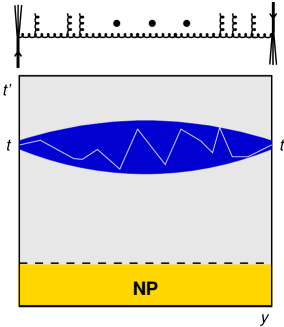
Figure 1: Above: a chain of emissions stretching in rapidity ($0<y<Y=\ln s/Q^{2}$) between the two hard probes at scale $t=\ln Q^{2}/\Lambda^{2}$. Below a schematic representation of typical transverse scales at different stages along the chain: the white line illustrates a typical random walk in $t^{\prime}$ ($\ln k^{2}$) as one goes along the chain, while the dark (blue) ‘cigar’ represents the average limits of this diffusion.

While at its ends the cigar is restricted to being narrow (by the presence of the probes), in the middle its width grows as a function of the centre of mass energy: $\Delta t^{\prime}\sim\sqrt{{\bar{\alpha}}_{\mathrm{s}}Y}$ with $Y=\ln s/Q^{2}$. For the problem to remain perturbative, typical trajectories must remain well outside the non-perturbative infrared region and this leads to the requirement that the width of the cigar be less than $t$, i.e. $\sqrt{{\bar{\alpha}}_{\mathrm{s}}Y}\ll t$. Using ${\bar{\alpha}}_{\mathrm{s}}(t)=1/bt$, with $b=11/12$ the coefficient of the $1$-loop $\beta$ function, this reduces to the condition $Y\ll bt^{3}$. This limit was originally derived (with some additional numerical factors) in [17, 18, 19, 20].

This picture of diffusion has its roots in the fixed-coupling approximation. It is tempting to consider the full running-coupling case as a small variation of the fixed-coupling situation. One then expects the differences to be that the centre of the cigar dips to $t^{\prime}$ values below $t$, and that the cigar profile in $t^{\prime}$ develops some asymmetry with respect to its centre (the cigar becomes a ‘banana’, figure 2a). This approach to the running-coupling case as a perturbation of the fixed-coupling case leads also to well-defined analytical predictions [18, 19, 20, 21]. In particular, the usual fixed-coupling exponential growth of the cross section, $\log\sigma\sim\alpha_{\mathrm{s}}Y$, is supplemented by an extra term proportional to $b^{2}\alpha_{\mathrm{s}}^{5}Y^{3}$. This can be interpreted as due to the centre of the cigar being at $t^{\prime}$ values of $t-{\cal O}\left(b\alpha_{\mathrm{s}}^{3}Y^{2}\right)$, which for $Y$ of order $bt^{2}$ implies that the cigar reaches the non-perturbative domain. Indeed calculations of the ‘purely perturbative’ component of the cross section show unphysical (oscillating) behaviour for $Y\gtrsim bt^{2}$, which can be interpreted as meaning that the perturbative component is not a physically well-defined quantity in that region [21, 22].

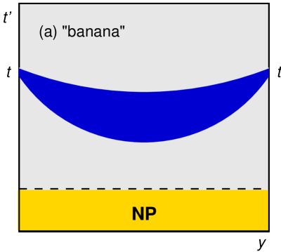
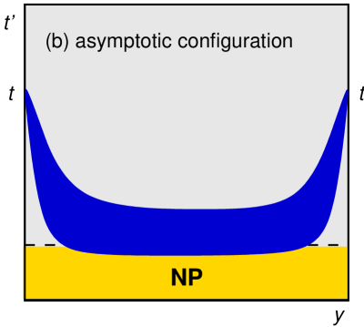
Figure 2: Analogues of fig. 1 which show the possible effects of the running coupling on the shape of the ‘cigar’.

Recently however, it was discovered in the context of a simplified, collinear model for BFKL dynamics [23], that the running of the coupling can introduce further qualitative differences. Rather than the width of the cigar gradually increasing with $Y$ until it reaches the non-perturbative region at $Y\sim bt^{3}$, or the centre of the cigar gradually moving in $t^{\prime}$ down until it reaches the non-perturbative region at $Y\sim bt^{2}$, it turns out that for $Y\sim t$ an abrupt transition occurs and the dominant trajectory switches from being centred around $t^{\prime}=t$ (fig. 1) to being centred around $t^{\prime}={\bar{t}}$, where ${\bar{t}}\gtrsim 0$ is in the non-perturbative region (fig. 2b). For such a transition, which we named ‘tunneling’, there is no passage through any intermediate ‘banana’ configuration (fig. 2a).

In this article we wish to explain this phenomenon in more detail than was done previously and for the case of the full BFKL equation with running coupling. In section 2 we present analytical calculations which give the estimate of the nonperturbative Pomeron, while in section 3 we illustrate the phenomenon with a number of figures resulting from the numerical solution of the BFKL equation.

2 Analytical considerations

It is useful to recall the form of the BFKL equation as we shall use it here. We define a BFKL Green’s function $G(Y,t,t_{0})$ through the following integro-differential equation

$$\frac{dG(Y,t,t_{0})}{dY}=\int\frac{d^{2}\vec{q}}{\pi q^{2}}\,{\bar{\alpha}}_{\mathrm{s}}(\ln q^{2})\left[\frac{k}{k^{\prime}}G(Y,\ln{k^{\prime}}^{2},t_{0})-G(Y,t,t_{0})\Theta(k-q)\right],\quad\begin{array}[]{l}k^{2}=e^{t}\,,\\ k^{\prime}=|\vec{k}+\vec{q}|\,,\end{array}$$ (1)

with the initial condition

$$G(0,t,t_{0})=\delta(t-t_{0})\,,$$ (2)

and with ${\bar{\alpha}}_{\mathrm{s}}=\alpha_{\mathrm{s}}N_{C}/\pi$. All scales are in units of $\Lambda_{\mathrm{QCD}}$. We shall take ${\bar{\alpha}}_{\mathrm{s}}$ as having its one-loop perturbative form, regularised by a cutoff at a non-perturbative scale ${\bar{t}}$:

$${\bar{\alpha}}_{\mathrm{s}}(t)=\frac{\Theta(t-{\bar{t}})}{bt}\,,\qquad b=\frac{11}{12}\,.$$ (3)

In some contexts we will use an equation similar to (1), but with $\alpha_{\mathrm{s}}(\ln q^{2})$ replaced by $\alpha_{\mathrm{s}}(t)$.

It will be convenient to define some high-energy exponents: $\omega_{\mathrm{s}}$, the perturbative saddle-point exponent, determines the high-energy behaviour of the Green’s function when it is dominated by scales of order $t$. It is given by $\omega_{\mathrm{s}}=(4\ln 2){\bar{\alpha}}_{\mathrm{s}}(t)+{\cal O}\left({\bar{\alpha}}_{\mathrm{s}}^{2}\right)$. We shall also need the non-perturbative pomeron exponent, $\omega_{\mathrm{I\!P}}$, which governs the asymptotic high-energy behaviour of the Green’s function, $G(Y)\sim\exp(\omega_{\mathrm{I\!P}}Y)$, once the problem has become dominated by non-perturbative scales. It is given by $\omega_{\mathrm{I\!P}}=(4\ln 2){\bar{\alpha}}_{\mathrm{s}}({\bar{t}})+{\cal O}\left(\smash{{\bar{\alpha}}_{\mathrm{s}}({\bar{t}})^{5/3}}\right)$, though it is to be kept in mind that the expansion in powers of ${\bar{\alpha}}_{\mathrm{s}}^{5/3}$ converges very slowly.

For the purpose of our arguments we shall take the formal perturbative limit of $t\gg{\bar{t}}$ and correspondingly $\omega_{\mathrm{s}}\ll\omega_{\mathrm{I\!P}}$.

2.1 Informal arguments for tunneling

The mechanism of tunneling is illustrated in figure 2b. To establish when tunneling takes place we have to equate the contribution from the tunneling configuration with that from the traditional perturbative configuration. Neglecting all prefactors, the tunneling configuration gives a contribution

$$G_{\mathrm{tunnel}}\sim e^{-(t-{\bar{t}})/2}\,e^{\omega_{\mathrm{I\!P}}Y}\,e^{-(t-{\bar{t}})/2},$$ (4)

corresponding (reading from left to right) to the ‘penalty’ for branching from $t$ to ${\bar{t}}$, the BFKL evolution at ${\bar{t}}$ and the penalty for branching back to $t$. In contrast, the perturbative contribution is proportional to

$$G_{\mathrm{pert}}\sim e^{\omega_{\mathrm{s}}Y}.$$ (5)

Equating these two expressions gives

$$Y_{\mathrm{tunnel}}(t)=\frac{t-{\bar{t}}}{\omega_{\mathrm{I\!P}}-\omega_{\mathrm{s}}(t)}\,.$$ (6)

Perhaps the most important characteristic of this equation is the fact that $Y_{\mathrm{tunnel}}$ is proportional to $t$ rather than $t^{3}$ as for the diffusion mechanism. One possible exception is the case in which the Pomeron is weak, that is $\omega_{\mathrm{I\!P}}\ll 1$. Then ${\bar{t}}$ should be quite large, and including in Eq.(6) the value $\omega_{\mathrm{s}}(t)=\chi_{m}/(bt)$ and the rough estimate $\omega_{\mathrm{I\!P}}=\chi_{m}/(b{\bar{t}})$ yields $Y_{\mathrm{tunnel}}=(bt/\chi_{m}){\bar{t}}$, so that the perturbative regime is kept up to $\omega_{\mathrm{s}}(t)Y$ values of order ${\bar{t}}$.

2.2 Formal arguments

For an isolated Pomeron “bound state”, the tunneling probability is estimated on the basis of the approximate decomposition

$$G(Y;t,t_{0})\;=\;G_{\rm pert}(Y;t,t_{0})+e^{\omega_{\mathrm{I\!P}}Y}\frac{{\cal F}_{\omega_{\mathrm{I\!P}}}(t){\cal F}_{\omega_{\mathrm{I\!P}}}(t_{0})}{\int dt{{\cal F}_{\omega_{\mathrm{I\!P}}}(t)}^{2}}\,,$$ (7)

where ${\cal F}_{\omega_{\mathrm{I\!P}}}(t)$ is the regular solution for $t\rightarrow\infty$ of the BFKL equation [24], satisfying the strong-coupling boundary condition also. The decomposition (7) separates the continuum from the lowest bound state contributions to the gluon’s Green functions [22] or, equivalently, the background integral from the leading Regge pole [21]. The normalisation of the bound state factor in front of $e^{\omega_{\mathrm{I\!P}}Y}$ is simply obtained by imposing that it be a projector by $t_{0}$ integration, or equivalently from the requirement that

$$G(Y;t,t_{0})=\int dt^{\prime}G(Y;t,t^{\prime})G(Y-y;t^{\prime},t_{0})\,.$$ (8)

Eq.(7) applies as it stands to a symmetrical BFKL kernel, as that with the scale choice ${\bar{\alpha}}_{\mathrm{s}}(\ln q^{2})$ in Eq.(1). If instead the scale ${\bar{\alpha}}_{\mathrm{s}}(t)$ is chosen, the kernel is asymmetrical, the conjugated wave function is $\bar{{\cal F}}_{\omega_{\mathrm{I\!P}}}(t)=t{\cal F}_{\omega_{\mathrm{I\!P}}}^{*}(t)$, and the bound state projectors differ by a $t_{0}$ factor and by the normalisation integral

$$G(Y;t,t_{0})\;=\;G_{\rm pert}(Y;t,t_{0})+e^{\omega_{\mathrm{I\!P}}Y}\frac{{\cal F}_{\omega_{\mathrm{I\!P}}}(t){\cal F}_{\omega_{\mathrm{I\!P}}}(t_{0})t_{0}}{\int dt\,t\,{{\cal F}_{\omega_{\mathrm{I\!P}}}(t)}^{2}}\,.$$ (9)

In either case, the large $t$ behaviour of ${\cal F}_{\omega_{\mathrm{I\!P}}}(t)$ is estimated in a semiclassical approach in which $b{\bar{\alpha}}_{\mathrm{s}}(t),1/Y$ and also $b\omega_{\mathrm{I\!P}}$ are taken to be small parameters (weak Pomeron, or $b$ - expansion [22]). In such a case the $\gamma$ - representation of ${\cal F}_{\omega_{\mathrm{I\!P}}}$ is valid, and takes the form

$${\cal F}_{\omega_{\mathrm{I\!P}}}(t)=\int_{1/2-i\infty}^{1/2+i\infty}\frac{d\gamma}{2\pi i}e^{(\gamma-1/2)t-\frac{1}{b\omega_{\mathrm{I\!P}}}X_{\omega_{\mathrm{I\!P}}}(\gamma)}\\ \simeq\sqrt{\frac{b\omega_{\mathrm{I\!P}}}{-2\pi\chi^{\prime}[p(b\omega_{\mathrm{I\!P}}t)]}}\exp\left[-\frac{1}{b\omega_{\mathrm{I\!P}}}\int_{\chi_{m}}^{b\omega_{\mathrm{I\!P}}t}p(x)\,dx\right]\;,$$ (10)

where the saddle point condition at $\bar{\gamma}=\frac{1}{2}-p$

$$\chi\left(\frac{1}{2}-p\right)\;=\;\frac{\partial X(\gamma)}{\partial\gamma}\bigg{|}_{\gamma=\frac{1}{2}-p}\;=\;b\,\omega_{\mathrm{I\!P}}t\;,$$ (11)

defines the semiclassical “momentum” $p(b\omega_{\mathrm{I\!P}}t)$. The effective eigenvalue function in Eq.(11) is just the leading characteristic function $\chi_{0}(\gamma)$ for the ${\bar{\alpha}}_{\mathrm{s}}(t)$ choice, and differs by some corrections involving the parameter $\omega_{\mathrm{I\!P}}$ in the symmetric scale choice ${\bar{\alpha}}_{\mathrm{s}}(\ln q^{2})$ which essentially lead to a rescaling of the (right) regular solution by a constant factor $\sim 1/\sqrt{\chi_{m}}$ (see Appendix) .

The Pomeron suppression arising from Eq.(10) has a universal form $\sim e^{\left(-\frac{1}{b{\bar{\alpha}}_{\mathrm{s}}(t)}g({\bar{\alpha}}_{\mathrm{s}}(t))\right)}$, where the function $g({\bar{\alpha}}_{\mathrm{s}})$ ($g(0)\neq 0$) is easily found from Eq.(11), [22]. On the other hand the perturbative part, corresponding to the continuum, is dominated by the saddle point exponent $\omega_{\mathrm{s}}(t)$

$$G_{\mathrm{pert}}(t,t_{0};Y)\;=\;\frac{1}{\sqrt{2\pi\chi_{m}^{{}^{\prime\prime}}{\bar{\alpha}}_{\mathrm{s}}(\frac{t+t_{0}}{2})Y}}\exp\left(\omega_{\mathrm{s}}\left(\frac{t+t_{0}}{2}\right)Y+\mathrm{corrections}\right)\;,$$ (12)

where the diffusion corrections are due to the running coupling [18, 19, 20].

From Eqs.(7,9,10) we estimate the $t$-dependence of the Pomeron contributions for the choices ${\bar{\alpha}}_{\mathrm{s}}(k^{2})$ (${\bar{\alpha}}_{\mathrm{s}}(q^{2})$) of the running coupling scale respectively

$$G_{\mathrm{I\!P}}^{(k)} = \frac{N^{(k)}({\bar{t}})}{2\pi b\omega_{\mathrm{I\!P}}t}\exp\left[-t+\frac{2}{\omega_{\mathrm{I\!P}}}\left(\log b\omega_{\mathrm{I\!P}}t+1+\psi(1)+{\cal O}\left(\frac{1}{(b\omega_{\mathrm{I\!P}}t)^{3}}\right)\right)\right]\,,$$

$$G_{\mathrm{I\!P}}^{(q)} = \frac{N^{(q)}({\bar{t}})}{2\pi(b\omega_{\mathrm{I\!P}}t)^{2}}\left(\frac{b\omega_{\mathrm{I\!P}}}{\chi_{m}}\right)\exp\left[-t+\frac{2}{\omega_{\mathrm{I\!P}}}\left(\log b\omega_{\mathrm{I\!P}}t+1+\psi(1)+{\cal O}\left(\frac{1}{(b\omega_{\mathrm{I\!P}}t)^{3}}\right)\right)\right]\,.$$

Notice that they differ both in the $t$-dependence, because of the $t$ factor on Eq.(9) and for the ${\bar{t}}$-dependent normalisation integrals

$$N^{(k)}({\bar{t}})=\left(\int_{{\bar{t}}}^{\infty}dt\,t\,{\cal F}_{\omega_{\mathrm{I\!P}}}^{2}(t)\right)^{-1}\,,$$

$$N^{(q)}({\bar{t}})=\left(\int dt{\cal F}_{\omega_{\mathrm{I\!P}}}^{2}(t)\right)^{-1}\,,$$ (14)

The latter quantities cannot be estimated in the semiclassical approximation, which breaks down at the turning points, and they need to be evaluated numerically. We can roughly estimate their size on the basis of the Airy diffusion model [24] obtained by the quadratic expansion of the characteristic function

$$\chi_{\omega}(\gamma)\;=\;\chi_{m}\;+\;\frac{1}{2}\chi_{m}^{\prime\prime}(\gamma-\gamma_{m})^{2}+\cdots\;.$$ (15)

This approximation is expected to be a reliable one for the Pomeron dynamics provided the fluctuations $\langle(\gamma-\gamma_{m})^{2}\rangle\sim\frac{2b\omega_{\mathrm{I\!P}}}{\chi^{\prime\prime}_{m}}$ are small compared to $4!\chi^{\prime\prime}_{m}/(2\chi_{m}^{(4)})$, and $t$ varies in a range for which

$$\xi_{\omega_{\mathrm{I\!P}}}(t)\;=\;\left(\frac{2b\omega_{\mathrm{I\!P}}}{\chi_{m}^{\prime\prime}}\right)^{\frac{1}{3}}\left(t-\frac{\chi_{m}}{b\omega_{\mathrm{I\!P}}}\right)\;,$$ (16)

is a parameter of order unity. In this case the BFKL equation with the choice ${\bar{\alpha}}_{\mathrm{s}}(k^{2})$ reduces, by Eq.(15) to a second-order differential equation in $t$ [24], and the cut-off condition for ${\bar{\alpha}}_{\mathrm{s}}(t)$ at $t={\bar{t}}$ (3) implies that the regular solution for $t\rightarrow-\infty$ must vanish at ${\bar{t}}$ , and for $t$ around ${\bar{t}}$ takes the following form

$$\left(\frac{\chi^{\prime\prime}_{m}}{2b\omega}\right)^{\frac{1}{3}}\tilde{{\cal F}}_{\omega}(t)\;=\;\pi\left[\mathrm{Bi}[\xi_{\omega}(t)]-\frac{\mathrm{Bi}[\bar{\xi}_{\omega}({\bar{t}})]}{\mathrm{Ai}[\bar{\xi}_{\omega}({\bar{t}})]}\mathrm{Ai}[\xi_{\omega}(t)]\right]\;,$$ (17)

while the regular solution for $t\rightarrow\infty$ becomes

$$\left(\frac{\chi^{\prime\prime}_{m}}{2b\omega}\right)^{\frac{1}{3}}{\cal F}_{\omega}(t)=\mathrm{Ai}\left[\xi_{\omega}(t)\right]\;,$$ (18)

with relative normalisation fixed by the Wronskian

$$\mathrm{W}({\cal F}_{\omega},\tilde{{\cal F}}_{\omega})=\frac{2b\omega}{\chi^{\prime\prime}_{m}}\;.$$ (19)

Using now the Airy form for the regular solution (18) we can evaluate the normalisation integrals (14) to get

$$N^{(k)}({\bar{t}}) = \frac{\chi_{m}}{b\omega_{\mathrm{I\!P}}}\left(\frac{2b\omega_{\mathrm{I\!P}}}{\chi_{m}^{{}^{\prime\prime}}}\right)^{\frac{1}{3}}\int_{-\xi_{0}}^{\infty}\!\!d\xi[\mathrm{Ai}(\xi)]^{2}+\int_{-\xi_{0}}^{\infty}\!\!d\xi\xi[\mathrm{Ai}(\xi)]^{2}=$$

$$= \xi_{0}[\mathrm{Ai}^{{}^{\prime}}(-\xi_{0})]^{2}\frac{\frac{2}{3}\omega_{\mathrm{s}}({\bar{t}})+\frac{1}{3}\omega_{\mathrm{I\!P}}}{\omega_{\mathrm{s}}({\bar{t}})-\omega_{\mathrm{I\!P}}}\,,$$

$$\chi_{m}N^{(q)}({\bar{t}}) = \left(\frac{2b\omega_{\mathrm{I\!P}}}{\chi_{m}^{{}^{\prime\prime}}}\right)^{\frac{1}{3}}\int_{-\xi_{0}}^{\infty}\!\!d\xi[\mathrm{Ai}(\xi)]^{2}=\xi_{0}\frac{\omega_{\mathrm{s}}({\bar{t}})}{\omega_{\mathrm{s}}({\bar{t}})-\omega_{\mathrm{I\!P}}}\frac{b\omega_{\mathrm{I\!P}}}{\chi_{m}}[\mathrm{Ai}^{{}^{\prime}}(-\xi_{0})]^{2}\,,$$ (20)

where we have used the Airy identities [25] and the assumption that the Pomeron intercept is given by the rightmost zero of the Airy $\mathrm{Ai}(\xi)$ function

$$\left(\frac{2b\omega_{\mathrm{I\!P}}}{\chi_{m}^{\prime\prime}}\right)^{\frac{1}{3}}\left({\bar{t}}-\frac{\chi_{m}}{b\omega_{\mathrm{I\!P}}}\right)\;=\;-\xi_{0}\simeq-2.3381\;,\hskip 28.45274pt\mathrm{Ai}(-\xi_{0})=0\;.$$ (21)

The additional factor $\chi_{m}$ which multiplies $N^{(q)}({\bar{t}})$ comes from the rescaling of the (right)regular eigenfunctions due to a scale change ${\cal F}^{(q)}_{\omega_{\mathrm{I\!P}}}(t)\sqrt{\chi_{m}}\simeq{\cal F}^{(k)}_{\omega_{\mathrm{I\!P}}}(t)$.

The expressions (2.2) supplemented by the normalisation factors (2.2) can be compared with the naive estimate (6) by rewriting them in the form

$$G_{\mathrm{I\!P}}^{(k)} = {\bar{\alpha}}_{\mathrm{s}}(t)\exp\left[-(t-{\bar{t}})+\frac{2}{b\omega_{\mathrm{I\!P}}}\log\frac{t}{{\bar{t}}}+\Delta^{(k)}\right]\;,$$

$$G_{\mathrm{I\!P}}^{(q)} = {\bar{\alpha}}_{\mathrm{s}}^{2}(t)\exp\left[-(t-{\bar{t}})+\frac{2}{b\omega_{\mathrm{I\!P}}}\log\frac{t}{{\bar{t}}}+\Delta^{(q)}\right]\;,$$ (22)

where one sees the explicit ${\bar{\alpha}}_{\mathrm{s}}(t)$, (${\bar{\alpha}}_{\mathrm{s}}(t)^{2}$) dependence for ${\bar{\alpha}}_{\mathrm{s}}(k^{2})$ and ${\bar{\alpha}}_{\mathrm{s}}(q^{2})$ scale choices respectively. The $\log\frac{t}{{\bar{t}}}$ in the exponent represents a collinear enhancement due to the evolution from scale $t$ to scale ${\bar{t}}$, and the ${\bar{t}}$ - dependent factors

$$\exp(\Delta^{(k)}) = \frac{1}{2\pi\xi_{0}[\mathrm{Ai}^{\prime}(-\xi_{0})]^{2}}\;\frac{[\omega_{\mathrm{s}}({\bar{t}})-\omega_{\mathrm{I\!P}}]}{\frac{1}{3}\omega_{\mathrm{I\!P}}+\frac{2}{3}\omega_{\mathrm{s}}({\bar{t}})}\;\frac{1}{\omega_{\mathrm{I\!P}}}\exp\left[\frac{2}{b\omega_{\mathrm{I\!P}}}(1+\psi(1)+\log b\omega_{\mathrm{I\!P}}{\bar{t}})-{\bar{t}}\right]\;,$$

$$\exp(\Delta^{(q)}) = \frac{\chi_{m}}{2\pi\xi_{0}[\mathrm{Ai}^{\prime}(-\xi_{0})]^{2}}\;\frac{[\omega_{\mathrm{s}}({\bar{t}})-\omega_{\mathrm{I\!P}}]}{\omega_{\mathrm{s}}({\bar{t}})\,\omega_{\mathrm{I\!P}}^{2}}\;\exp\left[\frac{2}{b\omega_{\mathrm{I\!P}}}(1+\psi(1)+\log b\omega_{\mathrm{I\!P}}{\bar{t}})-{\bar{t}}\right]\;,$$ (23)

come from the normalisation factors (2.2) and of the semiclassical prefactors. By then comparing the result (2.2) with the perturbative Green’s function in Eq.(12) we obtain the estimate of the tunneling transition rapidity in both scale choice cases

$$(\omega_{\mathrm{I\!P}}-\omega_{\mathrm{s}}(t))\,Y_{\mathrm{tunnel}}^{(k)} =t-{\bar{t}}-\frac{2}{b\omega_{\mathrm{I\!P}}}\log\frac{t}{{\bar{t}}}-\log{\bar{\alpha}}_{\mathrm{s}}(t)-\frac{1}{2}\log(2\pi\chi^{\prime\prime}_{m}{\bar{\alpha}}_{\mathrm{s}}(t)Y_{\mathrm{tunnel}})-\Delta^{(k)}({\bar{t}})\;,$$

$$(\omega_{\mathrm{I\!P}}-\omega_{\mathrm{s}}(t))\,Y_{\mathrm{tunnel}}^{(q)} =t-{\bar{t}}-\frac{2}{b\omega_{\mathrm{I\!P}}}\log\frac{t}{{\bar{t}}}-2\log{\bar{\alpha}}_{\mathrm{s}}(t)-\frac{1}{2}\log(2\pi\chi^{\prime\prime}_{m}{\bar{\alpha}}_{\mathrm{s}}(t)Y_{\mathrm{tunnel}})-\Delta^{(q)}({\bar{t}})\;,$$

2.3 Limits of the tunneling picture

We have just seen that the Pomeron regime sets in, according to Eqs.(6) and (LABEL:eq:YTunnelExact) at $\omega_{\mathrm{s}}(t)Y$ values of order ${\bar{t}}$. This is to be compared with the validity boundary of the hard Pomeron behaviour [22] $1\lesssim\omega_{\mathrm{s}}(t)Y\lesssim t/\sqrt{D}$, where $D=\frac{\chi^{\prime\prime}_{m}}{2\chi_{m}}$ is the diffusion coefficient. Thus, for phenomenological values of $t$ and ${\bar{t}}$ there appears to be little room for the hard Pomeron (and its diffusion corrections) to be observable, at least for models (such as the leading BFKL equation) in which the hard Pomeron and the nonperturbative Pomeron are quite strong. The Pomeron contamination in such cases, is a serious problem even for a theoretical determination of perturbative diffusion corrections to the hard Pomeron. In fact, one has to use the $b$-expansion [22] — $b\rightarrow 0$ limit with ${\bar{\alpha}}_{\mathrm{s}}(t)$ and ${\bar{\alpha}}_{\mathrm{s}}({\bar{t}})$ fixed — in order to identify such corrections at the numerical level.

The situation may change, if subleading and unitarity corrections are taken into account. Subleading contributions to the kernel are large [6] and need to be resummed [7, 8, 9]: they provide eventually a sizeable decrease of the hard Pomeron intercept and even more of the diffusion coefficient. This effect slows down both the nonperturbative effects and diffusion corrections, thus increasing the range of validity of the perturbative predictions. Furthermore, unitarity effects are expected to be important for large densities and more so in the strong coupling region. All this goes in the direction of a weaker asymptotic Pomeron — as is the actual physical Pomeron of soft physics [26] — thus increasing the effective ${\bar{t}}$ value, and the window of validity of the hard Pomeron regime.

It may thus be that in realistic small-$x$ models [14] with a weaker Pomeron, diffusion corrections to the hard Pomeron may set in before tunneling, so that the transition to the Pomeron regime is smoother. In any case, before diffusion corrections lead to a decreasing cross-section and to the asymptotic oscillatory regime[21] the Pomeron is expected to take over.

3 Pictorial results

3.1 Cigars

Perhaps the most dramatic illustration of the phenomenon of tunneling can be obtained through pictorial representations analogous to those of figures 1 and 2, but obtained by exact numerical solution of the BFKL equation.

This involves studying the running-coupling dynamics of BFKL evolution and in particular the sensitivity of the Green’s function $G(Y,t,t)$ to evolution at some intermediate point $y,t^{\prime}$. This can be done by examining:

$$f(Y,y,t,t^{\prime})=\frac{G(y,t,t^{\prime})G(Y-y,t^{\prime},t)}{G(Y,t,t)}\,,$$ (25)

which, by virtue of the linearity of the BFKL equation, is normalised as follows

$$\int dt^{\prime}f(Y,y,t,t^{\prime})=1\,.$$ (26)

From the point of view of graphical representation this quantity suffers from the problem that for $y\simeq 0$ or $y\simeq Y$ and $t^{\prime}\simeq t$ one is sensitive to the $\delta$-function initial condition for $G$, eq. (2). To smooth-out this $\delta$-function we examine instead a smeared version of $f$:

$${\bar{f}}(Y,y,t,t^{\prime})=\frac{\int dt_{0}\,dt_{1}\,e^{-(t_{0}-t)^{2}/2-(t_{1}-t)^{2}/2}\,G(y,t_{0},t^{\prime})G(Y-y,t^{\prime},t)}{\int dt_{0}\,dt_{1}\,e^{-(t_{0}-t)^{2}/2-(t_{1}-t)^{2}/2}\,G(Y,t_{0},t_{1})}$$ (27)

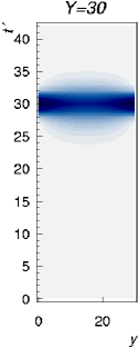
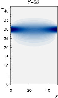
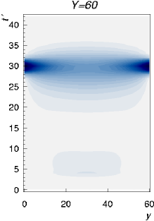
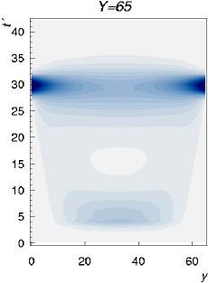
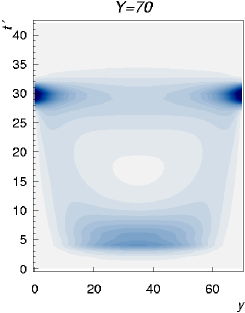
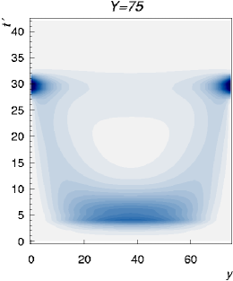
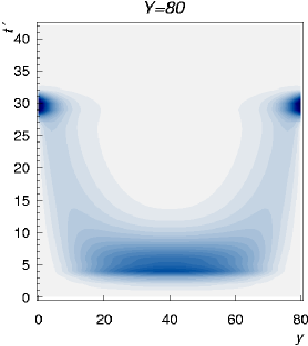
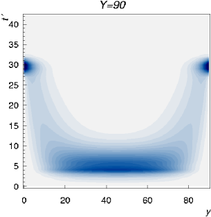
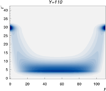
Figure 3: Contour plots for ${\bar{f}}(Y,y,t,t^{\prime})$, illustrating different stages of the evolution: $Y=30$ and $50$ illustrates standard ‘cigar’ type plots, $Y=60$–$70$ show the point where tunneling begins to play a role (BFKL ‘aliens’), while for $Y\gtrsim 80$ tunneling has become the dominant contribution (BFKL ‘bowls’). MPEG animations of the transition are available from http://www.lpthe.jussieu.fr/~​​​​salam/tunneling/ which includes additionally results for other combinations of $t$ and ${\bar{t}}$.

Contour plots of ${\bar{f}}(Y,y,t,t^{\prime})$ as a function of $y$ and $t^{\prime}$ are shown in figure 3 for various values of $Y$. We have chosen a value for $t$ that is physically unrealistic, $t=30$. The reason for this choice is that it enhances the separation between the perturbative and non-perturbative regions, allowing us to illustrate more clearly the transition that takes place. The coupling is regularised in the infrared, eq. (3), by a cutoff at ${\bar{t}}=4$.

At the lowest value of $Y$ in figure 3 the shape of the cigar is largely determined by the smearing of the initial condition, eq. (27). At $Y=50$ one can see a significant amount of diffusion at central values of $y$, as well as a slight asymmetry favouring lower $t^{\prime}$ values, caused by the running of the coupling.

At $Y=60$ the tunneling transition starts to take place: at low values of $t^{\prime}\simeq t$, an enhanced region appears which is disconnected from the main region of the cigar — it has not appeared through diffusion, but through tunneling. As $Y$ increases the perturbative region of $t^{\prime}\simeq t$ becomes progressively less important, eventually being completely supplanted by the non-perturbative region $t^{\prime}\simeq{\bar{t}}$. In this transition stage we take the liberty of referring to the contour plots as ‘BFKL aliens’.

Beyond $Y=75$, the evolution takes place entirely in the non-perturbative region, except in the wings, $y\simeq 0$ and $y\simeq Y$, which connect the initial conditions at $t$ to the infrared region. We refer to these contour plots as ‘bowls’.

We note that the position in $Y$ of the tunneling transition is quite consistent with the arguments of section 2. For our particular non-perturbative conditions, the non-perturbative power is $\omega_{\mathrm{I\!P}}\simeq 0.32$; substituting this into eq. (LABEL:eq:YTunnelExact) gives $Y_{\mathrm{tunnel}}\simeq 68$.

3.2 Ducks

 

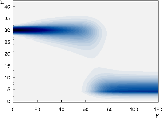
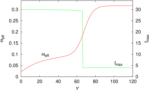
Figure 4: The upper figure is a contour plot of ${\bar{f}}(Y,Y/2,t,t^{\prime})$, corresponding to a cross section at $Y/2$ of ‘cigar’-type plots in fig. 3, as a function of $Y$. We refer to the resulting figure as a ‘duck’. The lower plot shows the effective exponent, $\omega_{\mathrm{eff}}$, and the position of the maximum of ${\bar{f}}$, $t_{\mathrm{max}}$, as a function of $Y$.

A convenient way of visualising the tunneling transition within a single plot is to consider ${\bar{f}}(Y,Y/2,t,t^{\prime})$ as a function of $Y$ and $t^{\prime}$, i.e. a contour plot built up of cross sections through the centres of the plots of figure 3, for a range of $Y$ values. This is shown in the upper plot of figure 4. At low $Y$ we see just the width of the initial condition, which gradually diffuses out while remaining centred at $t^{\prime}\simeq t$. At $Y\simeq 60$ a second region appears ‘out of nowhere’ at $t^{\prime}\simeq{\bar{t}}$ and the original cigar region disappears completely just beyond. This, once again, is the tunneling transition. We refer to the resulting figure as a ‘BFKL duck’.

In the lower plot of figure 4 we show two quantities as a function of $Y$ (on the same $Y$ scale as the upper plot): the effective exponent $\omega_{\mathrm{eff}}$, defined as

$$\omega_{\mathrm{eff}}=\frac{d}{dY}\ln\int dt_{0}\,dt_{1}\,e^{-(t_{0}-t)^{2}/2-(t_{1}-t)^{2}/2}\,G(Y,t_{0},t_{1})\,,$$ (28)

and the position of the maximum in $t^{\prime}$ of ${\bar{f}}(Y,Y/2,t,t^{\prime})$, which we refer to as $t_{\mathrm{max}}$. At the point where the tunneling transition occurs there is a jump in the value of $t_{\mathrm{\max}}$ as it switches from the perturbative to the non-perturbative region. Simultaneously there is a rapid change in $\omega_{\mathrm{eff}}$ as it goes from the perturbative exponent $\simeq\omega_{\mathrm{s}}$ to the non-perturbative one $\omega_{\mathrm{I\!P}}$.

We can use the point where the position of the maximum goes from being above to below $t^{\prime}=\frac{1}{2}(t+{\bar{t}})$ as the definition of where tunneling occurs, $Y_{\mathrm{tunnel}}$ (in what follows, since we will no longer be faced with the problem of visualising an initial $\delta$-function, we will actually consider $f(Y,Y/2,t,t^{\prime})$ rather than ${\bar{f}}$, though the difference in practice is minimal). Alternatively one can define the tunneling transition as occurring when the integrals of $f(Y,Y/2,t,t^{\prime})$ above and below $\frac{1}{2}(t+{\bar{t}})$ are equal,

$$\int^{(t+{\bar{t}})/2}_{-\infty}dt^{\prime}f(Y,Y/2,t,t^{\prime})=\int_{(t+{\bar{t}})/2}^{\infty}dt^{\prime}f(Y,Y/2,t,t^{\prime})\,.$$ (29)

These two definitions for $Y_{\mathrm{tunnel}}$ have been used to deduce, from our numerical solutions, the points with errors bars in fig. 5 (the lower error bar corresponds to the first definition, while the upper error bar corresponds to the second one), where we plot $Y_{\mathrm{tunnel}}$ as a function of $t$, for two values of ${\bar{t}}$. They are to be compared to the smooth lines, which correspond to the analytical predictions both in ${\bar{\alpha}}_{\mathrm{s}}(t)$ and ${\bar{\alpha}}_{\mathrm{s}}(\ln q^{2})$ cases. We have tried the direct evaluation of the $G_{\mathrm{I\!P}}$ from Eqs.(7), (9) by numerically calculating the $\gamma$-representation integrals (solid lines) and the analytical approximation based on the Airy model Eq. (LABEL:eq:YTunnelExact) (dashed lines).

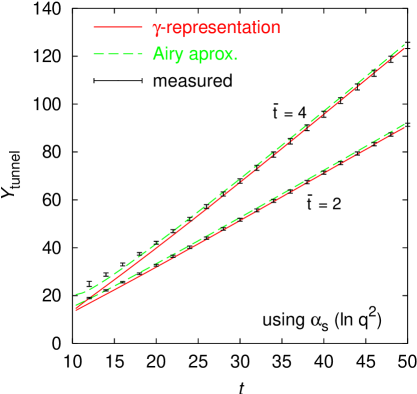
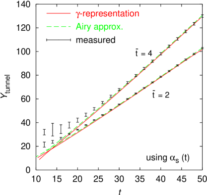
Figure 5: The position in $Y$ of the tunneling transition, $Y_{\mathrm{tunnel}}$ as a function of $t$ for two different non-perturbative cutoffs ${\bar{t}}$ (points). The points represent the numerical ‘measurements’ of $Y_{\mathrm{tunnel}}$ based on the criteria discussed in the text. They are compared to the prediction of Eq. (LABEL:eq:YTunnelExact), dashed lines and the calculation which involves the direct numerical evaluation of the $\gamma$-representation in the normalisation integrals Eq. (14), solid lines. Left-hand plot: the calculation for ${\bar{\alpha}}_{\mathrm{s}}(\ln q^{2})$ scale choice, right-hand plot: ${\bar{\alpha}}_{\mathrm{s}}(\ln k^{2})$.

One sees a remarkable agreement between the ‘numerically measured’ and analytical results, which would seem to be strong confirmation of even the fine details of our picture. We note in particular the roughly linear dependence of $Y_{\mathrm{tunnel}}$ on $t$ and the fact that its slope increases for larger ${\bar{t}}$ as a consequence of the smaller $\omega_{\mathrm{I\!P}}$ and hence smaller denominator in eq. (6).

4 Conclusions

In this paper we have presented a detailed investigation of the abrupt tunneling transition from the perturbative regime to the non-perturbative ‘Pomeron’ regime for the case of leading-log BFKL evolution with a running coupling.

The tunneling transition takes place when $\omega_{\mathrm{s}}Y\simeq{\bar{t}}$, with $\exp({\bar{t}})$ the effective non-perturbative scale of the problem (in units of $\Lambda^{2}_{QCD}$). This is parametrically much earlier than estimates of the maximum perturbatively accessible $Y$ value that are based on diffusion arguments. Furthermore, in contrast to expectations from diffusion arguments, the transition does not involve evolution at scales intermediate between those of the hard probe and the non-perturbative region, as shown in figs. 3 and 4.

Since the purpose of this paper has been to give an illustration of the effect of tunneling, we have restricted ourselves to leading-logarithmic evolution and considered only very extreme scales for the hard-probe, where the effect is more dramatic because of the large ratio $\omega_{\mathrm{I\!P}}/\omega_{\mathrm{s}}(t)$, or equivalently $t/{\bar{t}}$.

In a more phenomenologically relevant context there remain a number of other important issues: the separation between tunneling and diffusion may be less distinct, both because the accessible range of $t$ is smaller, and because for a given ratio of $t/{\bar{t}}$ higher-order corrections tend to reduce $\omega_{\mathrm{I\!P}}/\omega_{\mathrm{s}}(t)$. Furthermore unitarity and saturation corrections may actually cause the effective value of $\omega_{\mathrm{I\!P}}$ to be smaller than $\omega_{\mathrm{s}}$ which could eliminate tunneling altogether. Developing a better understanding of these and related questions remains one of the main challenges of small-$x$ physics.

Appendix A: Pomeron weight with $\boldsymbol{{\bar{\alpha}}_{\mathrm{s}}(\ln q^{2})}$

Taking ${\bar{\alpha}}_{\mathrm{s}}(\ln q^{2})$ instead of ${\bar{\alpha}}_{\mathrm{s}}(t)$, as in Eq.(1) means adding a term $-\frac{b}{2}(\chi^{\prime}_{0}+\chi_{0}^{2})$ to the NL kernel which emerges due to the evolution from scale $t$ to scale $q^{2}$. Correspondingly, in the $\omega$ - expansion formulation [8, 9] the effective characteristic function becomes

$$\chi_{\omega}=\chi_{0}(\gamma)+\omega\frac{1}{\chi_{0}}\left[-\frac{b}{2}(\chi^{\prime}_{0}+\chi_{0}^{2})\right]=\chi_{0}(\gamma)\left(1-\frac{b\omega}{2}\right)-\frac{b\omega}{2}\frac{\chi^{\prime}_{0}}{\chi_{0}}\;,$$ (30)

so that

$$X_{\omega}(\gamma)=\left(1-\frac{b\omega}{2}\right)\left[\log\left(\frac{\Gamma(1-\gamma)}{\Gamma(1+\gamma)}\gamma\right)+2\psi(1)\left(\gamma-\frac{1}{2}\right)\right]-\frac{b\omega}{2}\log\frac{\chi_{0}(\gamma)}{\chi_{0}(\frac{1}{2})}\;.$$ (31)

As a consequence, the large $t$-anomalous dimension stays the same

$$b\omega t=\chi_{\omega}(\bar{\gamma})\simeq\frac{1}{\bar{\gamma}}\;.$$ (32)

but the saddle point exponent $\log(\frac{G_{\mathrm{I\!P}}^{(q)}}{N(\omega_{\mathrm{I\!P}},{\bar{t}};t)})$ in (2.2) changes

$$-t+\frac{2}{b\omega_{\mathrm{I\!P}}}-\frac{2}{b\omega_{\mathrm{I\!P}}}\left\{\left[\log\left(\bar{\gamma}\frac{\Gamma(1-\bar{\gamma})}{\Gamma(1+\gamma)}\right)+2\psi(1)(\bar{\gamma}-\frac{1}{2})\right]\left(1-\frac{b\omega_{\mathrm{I\!P}}}{2}\right)-\frac{b\omega_{\mathrm{I\!P}}}{2}\log\frac{\chi_{m}(\bar{\gamma})}{\chi_{m}}\right\}\\ \simeq-t+\frac{2}{b\omega_{\mathrm{I\!P}}}\left[1+\psi(1)+\log b\omega_{\mathrm{I\!P}}t-\frac{b\omega_{\mathrm{I\!P}}}{2}\log\chi_{m}+{\cal O}\left(\frac{1}{(b\omega_{\mathrm{I\!P}}t)^{2}}\right)\right]\;.$$ (33)

It implies that approximately the eigenfunctions ${\cal F}_{\omega_{\mathrm{I\!P}}}^{(q)}(t)$ get rescaled by the additional constant normalisation factor so that $\sqrt{\chi_{m}}{\cal F}_{\omega_{\mathrm{I\!P}}}^{(q)}\simeq{\cal F}_{\omega_{\mathrm{I\!P}}}^{(k)}$.

References

-
[1]
L. N. Lipatov, Sov. J. Nucl. Phys.
23 (1976) 338;
E. A. Kuraev, L. N. Lipatov, V. S. Fadin, Sov. Phys. JETP 45 (1977) 199;
I. I. Balitsky, L. N. Lipatov, Sov. J. Nucl. Phys. 28 (1978) 338. - [2] J. Kwieciński, Z. Phys. C29 (1985) 561.
- [3] J.C. Collins, J. Kwieciński Nucl. Phys. B316 (1989) 307.
- [4] J. Kwiecinski, A. D. Martin and J. J. Outhwaite, Eur. Phys. J. C 9 (1999) 611.
- [5] B. Andersson, G. Gustafson and H. Kharraziha, Phys. Rev. D 57 (1998) 5543.
-
[6]
V. S. Fadin, M. I. Kotsky, R. Fiore,
Phys. Lett. B 359, (1995) 181;
V. S. Fadin, M. I. Kotsky, L. N. Lipatov, BUDKERINP-96-92, hep-ph/9704267;
V. S. Fadin, R. Fiore, A. Flachi, M. I. Kotsky, Phys. Lett. B 422, (1998) 287;
V. S. Fadin, L. N. Lipatov, Phys. Lett. B 429, (1998) 127;
G. Camici, M. Ciafaloni, Phys. Lett. B 386, (1996)341; Phys. Lett. B 412, (1997) 396 [Erratum-ibid. B 417, (1997)390 ]; Phys. Lett. B 430, (1998) 349. - [7] G. P. Salam, JHEP 9807 (1998) 019.
- [8] M. Ciafaloni, D. Colferai, Phys. Lett. B 452 (1999) 372.
- [9] M. Ciafaloni, D. Colferai and G. P. Salam, Phys. Rev. D 60 (1999) 114036.
- [10] G. Altarelli, R. D. Ball and S. Forte, Nucl. Phys. B 621 (2002) 359; G. Altarelli, R. D. Ball and S. Forte, Nucl. Phys. B 599 (2001) 383; G. Altarelli, R. D. Ball and S. Forte, Nucl. Phys. B 575 (2000) 313.
- [11] J. R. Forshaw, D. A. Ross and A. Sabio Vera, Phys. Lett. B 455 (1999) 273.
- [12] S. J. Brodsky, V. S. Fadin, V. T. Kim, L. N. Lipatov and G. B. Pivovarov, JETP Lett. 70 (1999) 155; V. S. Fadin, Nucl. Phys. A 666 (2000) 155.
- [13] C. R. Schmidt, Phys. Rev. D 60 (1999) 074003.
- [14] M. Ciafaloni, D. Colferai, G. P. Salam and A. M. Staśto, in preparation.
- [15] E. M. Levin, G. Marchesini, M. G. Ryskin and B. R. Webber, Nucl. Phys. B 357 (1991) 167.
- [16] J. Bartels and H. Lotter, Phys. Lett. B 309 (1993) 400.
- [17] A. H. Mueller, Phys. Lett. B 396 (1997) 251.
- [18] E. Levin, Nucl. Phys. B 453 (1995) 303;Nucl. Phys. B545 (1999) 481.
- [19] Y. V. Kovchegov and A. H. Mueller, Phys. Lett. B 439 (1998) 428.
- [20] N. Armesto, J. Bartels, M.A. Braun, Phys. Lett. B442 (1998) 459.
- [21] M. Ciafaloni, A. H. Mueller and M. Taiuti, Nucl. Phys. B 616 (2001) 349.
- [22] M. Ciafaloni, D. Colferai, G. P. Salam and A. M. Staśto, hep-ph/0204282.
- [23] M. Ciafaloni, D. Colferai and G. P. Salam, JHEP 9910 (1999) 017.
- [24] G. Camici, M. Ciafaloni, Phys. Lett. B395 (1997) 118.
- [25] I. S. Gradshtein, I. M. Ryzhik, Table of Integrals.
- [26] A. Donnachie, P.V. Landshoff, Phys. Lett. B296 (1992) 227.