Spontaneous chiral symmetry breaking in the linked cluster expansion

Abstract

We investigate dynamical chiral symmetry breaking in the Coulomb gauge Hamiltonian QCD. Within the framework of the linked cluster expansion we extend the BCS ansatz for the vacuum and include correlation beyond the quark-antiquark paring. In particular we study the effects of the three-body correlations involving quark-antiquark and transverse gluons. The high momentum behavior of the resulting gap equation is discussed and numerical computation of the chiral symmetry breaking is presented.

I Introduction

Chiral symmetry plays a major role in constraining the spectrum of low energy QCD. At zero density it is spontaneously broken and the associated Goldstone bosons dominate the low energy, soft hadronic interactions. The quark-gluon interactions which in vacuum break chiral symmetry may in dense matter, e.g. in the interior of neutron stars, lead to other, novel phases of the quark gluon plasma cf1 . The chiral properties of the QCD vacuum at zero temperature and density have been extensively studied in various approaches to soft QCD chsd ; chha ; Lis ; Cotan ; AA . In principle one could investigate it using lattice gauge methods. However, extrapolations of lattice simulations to small quark masses $m_{u,d}<<50-100\mbox{ MeV}$ (chiral extrapolation) still present a major challenge. In approaches bases on a Dyson-Schwinger formulation of QCD, dynamical chiral symmetry breaking can be studied by analyzing the behavior of the quark propagator. Even though no systematic truncation scheme of the Dyson series in QCD exists, and in a majority of studies model interactions are introduced, the approach gives a good description of the low energy phenomenology. In particular it enables to correctly predict many of the static properties of the low lying mesons and baryons, i.e. masses and charge moments, and simultaneously account for the dynamical chiral symmetry breaking as measured by the vacuum expectation value of the scalar quark density, $\langle{\bar{\psi}}\psi\rangle\sim-(250\mbox{ MeV})^{3}$ Maris . This value follows from PCAC, Goldstone theorem and the current algebra which result in the Gell-Mann-Oakes-Renner (or Thouless theorem) relation, $-2m_{q}\langle{\bar{\psi}}\psi\rangle=f_{\pi}^{2}m_{\pi}^{2}.$ Here, $m_{q}\sim 5-10\mbox{ MeV}$ is the current light quark mass, renormalized at the hadronic scale, $f_{\pi}=93\mbox{ MeV}$ is the pion decay constant and $m_{\pi}$ is the pion mass. Without explicit chiral symmetry breaking $m_{q}=0$, the above relation cannot be used to determine $\langle{\bar{\psi}}\psi\rangle$. However, as $m_{q}\to 0$ no phase transition to a chirally symmetric state is expected, and therefore the $~{}-(200-250\mbox{ MeV})^{3}$ should still be a good estimate of the condensate in the chiral limit.

Spontaneous chiral symmetry breaking enables to put the constituent quark representation of hadrons in a firm theoretical ground. The bare quark states defined with respect to the perturbative vacuum are replaced by quasiparticle excitations of the chirally noninvariant ground state. Residual interactions correlate the quasiparticles to form composite hadrons in which each valence quasiparticle contributes kinetic energy of the order of a few hundred MeV. This is analogous to the constituent quark model representation of hadrons and therefore it might be possible to further constraint the quark model phenomenology from a first principle, QCD based analysis of dynamical chiral symmetry breaking. Since the quark model picture calls for a Fock space representation it is most natural to consider a canonical, time-independent formulation of QCD. Coulomb gauge QCD offers such a framework cl1 ; ss3 ; cl3 . In the Coulomb gauge the single particle spectrum contains only physical degrees of freedom, i.e. two transverse gluon polarizations. As long as the gauge fields are restricted to the fundamental modular region, with no Gribov copies, the Hamiltonian is positively defined, it leads to a continuous time evolution, and it is amenable to a variational treatment. Finally the Coulomb gauge formulation leads to a natural realization of confinement. This arises because elimination of the non-physical degrees of freedom through the gauge choice, ${\nabla\cdot{\bf A}}=0$ results in an effective, long ranged instantaneous interaction between color charges. This interaction is the analog of the Coulomb potential in QED. In QCD however, the colored Coulomb gluons can couple to transverse gluons leading to a Coulomb kernel which also depends on the dynamical gluon degrees of freedom. As shown in Ref. ss7 summation of the dominant IR contributions to the vacuum expectation value of the Coulomb operator results in a potential between color charges which grows linearly at large distances in agreement with lattice calculations latt1 . In a self-consistent treatment the same potential modifies the single gluon spectral properties and leads to an effective mass for quasi-gluon excitations $~{}O(500-800\mbox{ GeV})$, which is also in agreement with recent lattice calculations. The appearance of the gluon mass gap can be used to justify the implicit assumption of the quark model that mixing between valence quarks and Fock space sectors with explicit gluonic excitations is small. We will return to this point in Section III.

The Coulomb gauge formulation provides a very natural starting point for building the constituent representation in accord with confinement and dynamical chiral symmetry breaking. However, as it was noticed some time ago in the Coulomb gauge the simple BCS treatment of the vacuum is not sufficient to generate the right amount of chiral symmetry breaking. In particular if a pure linear potential is used, $V(r)=br$ with $b\sim 0.2-0.25\mbox{ GeV}^{2}$ as determined by lattice calculations one typically obtains $|\langle{\bar{\psi}}\psi\rangle|^{1/3}\sim 100\mbox{ MeV}$ i.e. too small by a factor of two AA ; chha ; Cotan . The short range part of the Coulomb potential requires proper handling of UV divergences and renormalization and in most recent studies has been ignored. As will be shown later, it does significantly enhance the condensate and we will argue that the missing contribution can be accounted for by three-particle correlations on top of the BCS-like, particle-hole vacuum.

The paper is organized as follows. In Section II we briefly discuss the canonical Coulomb gauge formalism and the linked cluster expansion which enables to include multi-particle correlations into the many-body ground state. We will derive the resulting contributions to the mass gap including up to three-body correlations. The formalism is suitable for handling both zero and finite density system and in this paper we will focus on the former. In Section III we discuss the approximations, numerical results and possible sources of UV divergence and their renormalization. Our conclusions and outlook are given in Section IV.

II Coulomb gauge Hamiltonian and the linked cluster expansion

QCD canonically quantized in a physical gauge, e.g. Coulomb gauge, results in a Hamiltonian that can be represented in a complete Fock space defined by a set of single particle orbitals. One possibility is to choose the single particle basis as eigenstates of the kinetic (noninteracting) part of the full Hamiltonian,

$$H_{0} = H(g=0)=\int d{\bf x}\psi^{{\dagger}}({\bf x})\left[-i\bbox{\alpha}\cdot\nabla+\beta m\right]\psi({\bf x})$$ (1)

$$+\int d{\bf x}\left[\mbox{Tr }\bbox{\Pi}({\bf x})^{2}+\mbox{Tr }\left({\bf\nabla}\times{\bf A}({\bf x})\right)^{2}\right].$$

The vacuum, $|0\rangle$, of $H_{0}$ is shown schematically in Fig. 1a. The singe-particle excitations at zero density correspond to adding gluons to the positive energy, parton-like levels and quark-antiquark paris by creating a particle-hole excitation around the zero-energy Fermi surface. These excitations have energies given by, $\epsilon^{0}_{q}({\bf k})=\epsilon^{0}_{\bar{q}}({\bf k})=\sqrt{m^{2}+{\bf k}^{2}}$, $\epsilon^{0}_{g}({\bf k})=|{\bf k}|$ for quarks, antiquarks and gluons, respectively. The quark fields in Eq. (1) satisfy the canonical anticommutation relations and the gluons fields are given by $\bbox{\Pi}\equiv\bbox{\Pi}^{a}T^{a}$ and ${\bf A}\equiv{\bf A}^{a}T^{a}$ and satisfy the canonical commutation relations for transverse fields, i.e.

$$\left[\bbox{\Pi}^{a}({\bf x}),{\bf A}^{b}({\bf y})\right]=-i\delta^{ab}\bbox{\delta}_{T}(\nabla)\delta^{3}({\bf x}-{\bf y}),$$ (2)

where $\bbox{\delta}_{T}(\nabla)=I-\bbox{\nabla}\otimes\bbox{\nabla}/\bbox{\nabla}^{2}$. In terms of the single particle creation and annihilation operators, the color triplet of quark fields ($i=1,2,3$) is given by,

$$\psi_{i}({\bf x})=\sum_{\lambda=\pm 1/2}\int{{d{\bf k}}\over{(2\pi)^{3}}} \left[u({\bf k},\lambda)b({\bf k},\lambda,i)\right.$$

$$\left.+v(-{\bf k},\lambda)d^{{\dagger}}(-{\bf k},\lambda,i)\right]e^{i{\bf k}\cdot{\bf x}},$$

where $u$ and $v$ are solution of the free Dirac equation for a fermion with mass $m$. In the following we will restrict our discussion to chirally symmetric case i.e. from now on we will set $m=0$. The gluon field is given by,

$${\bf A}^{a}({\bf x})=\sum_{\lambda=\pm 1}\int{{d{\bf k}}\over{(2\pi)^{3}}} {1\over\sqrt{2\omega^{0}({\bf k})}}\left[a({\bf k},\lambda,a)\bbox{\epsilon}({\bf k},\lambda)\right.$$

$$\left.+a^{{\dagger}}(-{\bf k},\lambda,a)\bbox{\epsilon}^{*}(-{\bf k},\lambda)\right]e^{i{\bf k}\cdot{\bf x}},$$

with $\omega^{0}({\bf k})=\epsilon^{0}_{g}(|{\bf k}|)$. The unrenormalized Coulomb operator is given by,

$$H_{C}={g^{2}\over 2}\int d{\bf x}d{\bf y}\rho^{a}({\bf x})K_{ab}({\bf x},{\bf y},{\bf A})\rho^{b}({\bf y}),$$ (5)

where $\rho^{a}({\bf x})=\psi^{{\dagger}}({\bf x})T^{a}\psi({\bf x})+f^{abc}\bbox{\Pi}^{b}({\bf x})\cdot{\bf A}^{c}({\bf x})$ is the color charge density and the kernel $K$ is given by,

$$K_{ab}({\bf x},{\bf y},A)=\langle{\bf x},a|{1\over{\bbox{\nabla}\cdot{\bf D}}}(-\bbox{\nabla}^{2}){1\over{\bbox{\nabla}\cdot{\bf D}}}|{\bf y},b\rangle,$$ (6)

where ${\bf D}$ is the covariant derivative in the adjoint representation, and the $\langle{\bf x},a|\cdots|{\bf y},b\rangle$ matrix element is given by $\langle{\bf x},a|{\bf D}|{\bf y},b\rangle=\left[\delta^{ab}\bbox{\nabla}_{{\bf x}}+gf^{acb}{\bf A}^{c}({\bf x})\right]\delta^{3}({\bf x}-{\bf y})$, and $\langle{\bf x},a|1/\bbox{\nabla}^{2}|{\bf y},b\rangle=-1/4\pi|{\bf x}-{\bf y}|$. When $H_{C}$ is normal ordered with respect to the perturbative vacuum, $|0\rangle$ one might expect that the mean field, Hartee-Fock corrections to the single particle energies could already generate an effective mass. This is not the case. The vacuum is a color singlet and thus the direct contribution from $H_{C}$ to a single fermion energy vanishes. Furthermore, chiral symmetry of the Hamiltonian and of the perturbative, $|0\rangle$ vacuum protects the exchange term from mass generation. The effective mass can only be obtained if quark-antiquark correlations are introduced into the ground state as shown schematically in Fig. 1b.

Figure 1: Schematic representation of the particle, $n^{+}\equiv\langle b^{{\dagger}}b\rangle$ (solid) and hole $n^{-}\equiv 1-\langle d^{{\dagger}}d\rangle$ (dashed) occupations in partonic (left) and BCS (right) ground state

The full, unrenormalized Coulomb gauge Hamiltonian has the following structure cl3 ; ss7 ; CL ; swif ,

$$H=H_{0}+H_{C}+V_{qg}+V_{3g}+V_{4g}+H_{corr}.$$ (7)

Here $V_{qg}$ is the quark-transverse gluon interaction,

$$V_{qg}=g\int d{\bf x}\psi^{{\dagger}}({\bf x})\bbox{\alpha}\cdot{\bf A}\psi({\bf x}),$$ (8)

and $V_{3g}$ and $V_{4g}$ represent 3– and 4– transverse gluon couplings arising from the nonabelian part of the magnetic field, ${\bf B}^{a}=\nabla\times{\bf A}^{a}+gf^{abc}{\bf A}^{b}({\bf x})\times{\bf A}^{c}({\bf x})$. Finally $H_{corr}$ contains terms which come from a commutator of the determinant of the Faddeev-Popov operator, ${\cal J}=Det({\bbox{\nabla}\cdot{\bf D}})$ and the gluon canonical momentum $\bbox{\Pi}$. The detailed analysis of this Hamiltonian, emergence of confinement and issues related to renormalization in the gluon sector were discussed in Ref. ss7 .

II.1 Linked cluster expansion

Since the Fock space basis generated by the set of single particle creation operators, $b^{{\dagger}}$, $d^{{\dagger}}$, $a^{{\dagger}}$ is complete, the true ground state, $|\Omega\rangle$ of $H$ can be written as,

$$|\Omega\rangle=\left[1+\sum_{12}F^{(q{\bar{q}})}_{12}b^{{\dagger}}_{1}d^{{\dagger}}_{2}+\sum_{12}F^{(gg)}_{12}a^{{\dagger}}_{1}a^{{\dagger}}_{2}+\sum_{123}F^{(q{\bar{q}}g)}_{123}b^{{\dagger}}_{1}d^{{\dagger}}_{2}a^{{\dagger}}_{3}+\sum_{1234}F^{(q{\bar{q}}q{\bar{q}})}_{1234}b^{{\dagger}}_{1}d^{{\dagger}}_{2}b^{{\dagger}}_{3}d^{{\dagger}}_{4}+\cdots\right]|0\rangle.$$ (9)

Here $F^{(n)}_{12\cdots n}$ represent wave functions of n-body clusters in the vacuum, and $1,2\cdots$ collectively denote quantum numbers of single particle orbitals. This expansion is however impractical since it does not differentiate between connected (linked) and disconnected contributions. For example, at the 2-quark-2-antiquark level there are disconnected contributions of the type, $F^{(q{\bar{q}}q{\bar{q}})}_{1234}=F^{(q{\bar{q}})}_{12}F^{(q{\bar{q}})}_{34}$, i.e. part of the $n$-particle cluster contribution originates from products of smaller, $m<n$, $m$-particle clusters.

The essence of the linked cluster expansion is based on the observation that all multi-particle correlation in the ground state, including the disconnected ones can be accounted for by proper resummation of the linked clusters only. This is achieved by writing the full ground state as exps

$$|\Omega\rangle=e^{-S}|0\rangle,$$ (10)

with $S$ having the expansion

$$S=\sum_{n}S^{(n)}=\sum_{12}S^{(q{\bar{q}})}_{12}b^{{\dagger}}_{1}d^{{\dagger}}_{2}+\sum_{12}S^{(gg)}_{12}a^{{\dagger}}_{1}a^{{\dagger}}_{2}+\sum_{123}S^{(q{\bar{q}}g)}_{123}b^{{\dagger}}_{1}d^{{\dagger}}_{2}a^{{\dagger}}_{3}+\sum_{1234}S^{(q{\bar{q}}q{\bar{q}})}_{1234}b^{{\dagger}}_{1}d^{{\dagger}}_{2}b^{{\dagger}}_{3}d^{{\dagger}}_{4}+\cdots,$$ (11)

with the operators $S$ including connected pieces only. Comparing Eq. (9) and Eq. (11) we find for example that,

$$F^{(q{\bar{q}})}_{12}=S^{(q{\bar{q}})}_{12},\;\;F^{(q{\bar{q}}g)}_{123}=S^{(q{\bar{q}}g)}_{123},\;\;$$

$$F^{(q{\bar{q}}q{\bar{q}})}_{1234}=S^{(q{\bar{q}}q{\bar{q}})}_{1234}+{1\over 2}S^{(q{\bar{q}})}_{12}S^{(q{\bar{q}})}_{34},\cdots$$ (12)

i.e. the general expansion of Eq. (9) is obtained with all disconnected contributions constrained by the connected ones. The expansion coefficients, $S^{(n)}_{12\cdots n}$ can be determined from the eigenvalue equation for $|\Omega\rangle$,

$$e^{S}He^{-S}|0\rangle=E_{\Omega}|0\rangle.$$ (13)

This equation projected onto the partonic Fock space basis leads to a set of equations for the amplitudes $S^{(n)}_{12\cdots n}$ and the ground state energy, $E_{\Omega}$,

$$\langle 0|e^{S}He^{-S}|0\rangle=E_{\Omega},\;\;\langle q_{1},q_{2},\cdots q_{n_{q}};{\bar{q}}_{1^{\prime}},{\bar{q}}_{2^{\prime}},\cdots{\bar{q}}_{n_{\bar{q}}};g_{1^{\prime\prime}},g_{2^{\prime\prime}},\cdots g_{n_{g}}|e^{S}He^{-S}|0\rangle=0,n_{q},n_{\bar{q}},n_{g}=1,2,\cdots.$$ (14)

In a nonrelativistic many-body system the Hamiltonian is typically a polynomial in the field operators. Since each $S^{(n)}$ contains only particle creation operators, the matrix elements of $e^{S}He^{-S}$ between an $n$-particle state and the free vacuum will involve only a finite number of terms arising from the expansion of the exponentials. For example in a typical case when $H=H_{0}+V$ with $H_{0}$ being a one body (e.g. kinetic) operator and $V$ a two-body potential one has,

$$e^{S}He^{-S}=H+[S,H]+\cdots+{1\over{4!}}[S,[S,[S,[S,H]]]].$$ (15)

In this case an approximation to Eq. (14), is fully specified by a number of clusters retained in $S$. This is, however, not the case for the relativistic system discussed here. The expansion of the Coulomb kernel leads to an infinite series of operators to all orders in the transverse gluon field. Thus an approximation to Eq. (14) consists of specifying which clusters are kept in the definition of $S$ and of a truncation scheme in evaluation of matrix elements of $e^{S}He^{-S}$.

The truncation of $S$ limits the number of quark-antiquark-gluon correlations build into the ansatz for the ground state. At first one might think that such a truncation would be hard to justify since any hadronic state, including the vacuum should have a large (infinite) number of partons. However, the first two terms in $S$, $S^{(q{\bar{q}})}$ and $S^{(gg)}$ change the single particle excitation spectrum and effectively replace the partonic basis by that of massive quasiparticles. This is known as the Thouless reparameterization BR and is equivalent to the BCS ansatz for the vacuum which contains two-body, quark-antiquark and gluon-gluon correlations. The BCS ansatz leads to the chiral gap, constituent mass for the quarks as well as effective mass for the transverse gluons. Iterative contributions of multiparticle states which determine the wave functions of larger clusters, $S^{(n)}$, $n>2$ are therefore suppressed by the quasiparticle energy gap. This gap is $O(400-600\mbox{ MeV})$ for quark-antiquark excitations and $O(500\mbox{ MeV}-800\mbox{ GeV})$ for a gluonic excitation. The former follows from the typical constituent quark mass and the later from the gluon spectrum in a presence of static color sources as calculated on the lattice latt1 and are consistent with explicit calculation using the BCS gluonic ansatz for the Hamiltonian ss7 . The transformation form the partonic to the quasiparticle basis, generated by $S^{(2)}$, proceeds as follows. The (unnormalized) quasiparticle, BCS vacuum $|\Omega_{BCS}\rangle$ is defined as,

$$|\Omega_{BCS}\rangle\equiv e^{-S^{(2)}}|0\rangle,$$ (16)

with,

$$S^{(2)}=S^{(q{\bar{q}})}+S^{(gg)}= \sum_{12}S^{(q{\bar{q}})}_{12}b^{{\dagger}}_{1}d^{{\dagger}}_{2}$$ (17)

$$+\sum_{12}S^{(gg)}_{12}a^{{\dagger}}_{1}a^{{\dagger}}_{2},$$

so that

$$|\Omega\rangle=e^{-\sum_{n>2}S^{(n)}}|\Omega_{BCS}\rangle.$$ (18)

A canonical transformation which maps the set of free particle operators $b,b^{{\dagger}},d,d^{{\dagger}},a,a^{{\dagger}}$ onto a set of quasiparticle operators $B,B^{{\dagger}},D,D^{{\dagger}},\alpha,\alpha^{{\dagger}}$ is defined by

$$B_{1}={1\over{\sqrt{1+|S^{(q{\bar{q}})}|^{2}}}}b_{1}+\sum_{2}{{S^{(q{\bar{q}})}_{12}}\over{\sqrt{1+|S^{(q{\bar{q}})}|^{2}}}}d^{{\dagger}}_{2},$$

$$D_{1}={1\over{\sqrt{1+|S^{(q{\bar{q}})}|^{2}}}}d_{1}-\sum_{2}b^{{\dagger}}_{2}{{S^{(q{\bar{q}})}_{21}}\over{\sqrt{1+|S^{(q{\bar{q}})}|^{2}}}},$$

$$\alpha_{1}={1\over{\sqrt{1-|S^{(gg)}|^{2}}}}a_{1}+\sum_{2}{{S^{(gg)}_{12}}\over{\sqrt{1-|S^{(gg)}|^{2}}}}a^{{\dagger}}_{2},$$ (19)

where $|S^{(q{\bar{q}})}|^{2}\delta_{12}\equiv\left[S^{(q{\bar{q}})}{S^{(q{\bar{q}})}}^{{\dagger}}\right]_{12}$ and similarly for $|S^{(gg)}|$. These quasiparticle operators satisfy the canonical (anti)commutation relations, they annihilate the BCS ground state,

$$B_{1}|\Omega_{BCS}\rangle=D_{1}|\Omega_{BCS}\rangle=\alpha_{1}|\Omega_{BCS}\rangle=0,$$ (20)

and generate a complete Fock space. The eigenvalue conditions for the vacuum, Eq (14) can therefore be rewritten in the quasiparticle basis,

$${{\langle\Omega_{BCS}|e^{S}He^{-S}|\Omega_{BCS}\rangle}\over{\langle\Omega_{BCS}|\Omega_{BCS}\rangle}}=E_{\Omega},\;\;\langle Q_{1},Q_{2},\cdots Q_{n_{Q}};{\bar{Q}}_{1^{\prime}},{\bar{Q}}_{2^{\prime}},\cdots{\bar{Q}}_{n_{\bar{Q}}};G_{1^{\prime\prime}},G_{2^{\prime\prime}}, \cdots G_{n_{G}}|e^{S}He^{-S}|\Omega_{BCS}\rangle=0,$$ (21)

$$n_{Q},n_{\bar{Q}},n_{G}=1,2,\cdots.$$

Here the operator $S$ contains contributions from 3-quasiparticle cluster and higher,

$$S=\sum_{123}{\tilde{S}}^{(Q{\bar{Q}}G)}_{123}B^{{\dagger}}_{1}D^{{\dagger}}_{2}\alpha^{{\dagger}}_{3}+\cdots.$$ (22)

The matrix elements ${\tilde{S}}^{(n)}_{12\cdots n}$ can be related to $S^{(n)}_{12\cdots n}$ by replacing the free particle operators by the quasiparticle operators. From the structure of Eq. (19) it follows that for given $n$ the operators ${\tilde{S}}^{(n)}$ are a linear combination of $S^{(i)}$ including $i\leq n$. Since Eq. (19) defines a canonical transformation the two sets of equations, Eq (14) and Eq. (21) are equivalent and one can simply use the later i.e. work directly in the quasiparticle basis without referring to the partonic basis. As suggested by the quark model it is preferred to represent low energy QCD eigenstates in terms of quasiparticle, quark and gluon excitations. From now on we will work the matrix elements of ${\tilde{S}}$ in the quasiparticle basis and for simplicity rename them as ${\tilde{S}}^{(n)}\to S^{(n)}$.

As mentioned earlier, in QCD, with $S=\sum_{n}S^{(n)}$ truncated at some maximal $n$, Eq. (21) still contain an infinite number of terms arising from the expansion of $e^{S}He^{-S}$. Since this (infinite) series is related to the multi-gluon structure of the Coulomb operator, $K({\bf x},{\bf y},{\bf A})$, it can be organized according to how each of the terms renormalizes the 0-th order Coulomb potential, $K_{ab}({\bf x},{\bf y},0)=\delta_{ab}/4\pi|{\bf x}-{\bf y}|$. To illustrate this consider truncating $S$ at $n=2$. The lhs. of the first equation in  (21) reduces to the expectation value of $H$ in the BCS vacuum,

$$\langle\Omega_{BCS}|e^{S}He^{-S}|\Omega_{BCS}\rangle=\langle\Omega_{BCS}|H|\Omega_{BCS}\rangle.$$ (23)

The lowest order (in the loop expansion) diagrams are shown on the left side of Fig. 2. The matrix element $\langle\Omega_{BCS}|H|\Omega_{BCS}\rangle$ defines an effective potential $V_{eff}({\bf x}-{\bf y})$, by

$$V_{eff}({\bf x}-{\bf y})\equiv g^{2}{{\delta_{ab}}\over{N_{c}^{2}-1}}\langle\Omega_{BCS}|K_{ab}({\bf x},{\bf y},{\bf A})|\Omega_{BCS}\rangle.$$ (24)

It is straightforward to identify diagrams which give the dominant contribution to $V_{eff}$ in both, the IR ($|{\bf x}-{\bf y}|>>1/\Lambda_{QCD}$) and the UV ($|{\bf x}-{\bf y}|<<1/\Lambda_{QCD}$). In the IR region these are given by diagrams which, at a given loop order contain the maximum number of soft potential, $K({\bf x},{\bf y},0)$ lines; the UV region is dominated by loops with the smallest number of vertices. The series of ring and rainbow diagrams, shown in Fig. 2, accounts for the leading IR and UV contributions to $V_{eff}$, respectively. The approximation can be systematically improved by taking into account the subleading contributions e.g. vertex renormalization ss7 ; swif

Figure 2: A few lowest order contributions to $V_{eff}$. The two right most diagrams represent diagrams in the ring and rainbow series. The dashed line stands for the 0-th order Coulomb potential $g^{2}K_{0}=g^{2}/4\pi|{\bf x}-{\bf y}|$.

If larger clusters in $S$ are retained, the expansion of $e^{S}He^{-S}$ generates operators that have nonvanishing matrix elements between the vacuum and states with an arbitrary large number of particles. This is because as long as $S^{(n)}$ contains a gluon operator an infinite number of commutators, $[S^{(n)},[S^{(n)},[\cdots[S^{(n)},H]\cdots]]]$ are nonvanishing. Their contribution arise from contracting gluons from each $S^{(n)}$ with gluons from the Coulomb operator. For example a term in $S$ which contains pure glue operators (no quark or antiquark) will contribute to any matrix element in Eq. (21) with any number of particles (gluons). This is illustrated in Fig. 3 for $S^{(3g)}$. It is clear, however, that this type of corrections have the effect of simply renormalizing $V_{eff}$, beyond the BCS-like contributions shown in Fig. 2. Since the operators $S^{(n)}$ commute with each other one possibility is to consider the effects of the pure gluon operators first, generate the new effective interaction and then introduce clusters which contain quark and antiquark operators. Since $H$ is a finite order polynomial in the quark operators, each term in $S$ containing only quark and antiquark operators will lead to a finite number of terms in a matrix element between the BCS vacuum and a multiparticle state with a fixed, $n=n_{Q}+n_{\bar{Q}}+n_{G}$.

Figure 3: Example of contributions to $[S^{(n)},[S^{(n)},[\cdots[S^{(n)},H]\cdots]]]$, for $S=S^{ggg}$ and $H=H_{C}$. The two diagrams contribute to a matrix element with $n_{G}=2$ and $n_{G}=4$ respectively. Here the dashed line represents the Coulomb potential dressed by the BCS corrections, Eq. (24), e.g. through resummation of the ring-rainbow series shown in Fig. 2.

To summarize, the linked cluster expansion of the QCD ground state is much more complicated that in a typical nonrelativistic many-body problem. Nevertheless it can be used to systematically improve the BCS approximation. It is important to notice, however, that even the BCS ground state already probes the nonabelian multi-gluon dynamics via $\langle\Omega_{BCS}|K({\bf x},{\bf y},{\bf A})|\Omega_{BCS}\rangle$. In BCS this leads to and effective interaction which is very close to the potential between color sources and when treated selfconsistently leads to a quasiparticle (constituent) representations.

II.2 $Q{\bar{Q}}G$ contribution to the quark mass gap

In the following we will concentrate on the dynamical chiral symmetry breaking and therefore consider vacuum properties in quark sector.

Figure 4: Operators from Eq. 27 which contribute to matrix elements $\langle n_{Q},n_{\bar{Q}},n_{G}|\cdots|\Omega_{BCS}\rangle$ for $n_{Q}\leq 1$, $n_{\bar{Q}}\leq 1$ and $n_{G}\leq 2$ As in Fig. 3, the potential (dashed) line is the $V_{eff}$ of Eq. (24). The matrix element, $\SS$ corresponds to the rightmost vertices.

As mentioned earlier the BCS mechanism of quark-antiquark pairing seems to be insufficient to account for the full dynamical symmetry breaking. We will discuss this point quantitatively in the following section. Our interest here is in extending the BCS approximation by including the effects of the next to leading (beyond BCS) order in the cluster expansion i.e. the 3–particle cluster contribution to the vacuum. We will therefore study,

$$S\to\SS=\sum_{123}\SS_{123}B^{{\dagger}}_{1}D^{{\dagger}}_{2}\alpha^{{\dagger}}_{3}.$$ (25)

The quark gap equation follows from,

$$\langle Q_{1}{\bar{Q}}_{2}|e^{\SS}He^{-\SS}|\Omega_{BCS}\rangle=0.$$ (26)

This equation determines single particle orbitals and therefore it also gives the quasiparticle spectrum via, $\epsilon_{1}\delta_{12}=\langle Q_{1}|H|Q_{2}\rangle$. There is a finite number of terms contributing to, Eq. (26)

$$0=\langle Q_{1}{\bar{Q}}_{2}|H+[\SS,H]+{1\over{2!}}[\SS,[\SS,H]]+{1\over{3!}}[\SS,[\SS,[\SS,H]]|\Omega_{BCS}\rangle.$$ (27)

The series is finite because starting at $O(\left[{\SS}\right]^{4}\sim\left[B^{{\dagger}}D^{{\dagger}}\right]^{4})$ commutators will produce operators which have at least 2-quark and 2-antiquark creation operators and these vanish between $\langle Q{\bar{Q}}|$ and $|\Omega_{BCS}\rangle$. Some of the contributions to Eqs. (27) and  (28) are shown in Fig. 4. In order to solve Eq. (27) and determine the single particle basis, it is necessary to first solve for the amplitude $\SS$. This amplitude can be obtained by projecting $e^{\SS}He^{-\SS}$ onto the three particle cluster,

$$\langle Q_{1}{\bar{Q}}_{2}G_{3}|H+[\SS,H]+{1\over{2!}}[\SS,[\SS,H]]+{1\over{3!}}[\SS,[\SS,[\SS,H]]]|\Omega_{BCS}\rangle=0,$$ (28)

which also contains a finite number of terms. The two equations Eq. (27) and Eq. (28) form a set of coupled nonlinear, integral equations for the amplitude $\SS$ and the single particle orbitals (or the BCS angle, Eq. (19)). In this paper we will simplify these equations by linearizing them with respect to $\SS$, Eq.( 28) then yields,

$$\SS|\Omega_{BCS}\rangle=\sum_{n}|n\rangle{1\over{E_{n}-E_{\Omega_{BCS}}}}\langle n|H|\Omega_{BCS}\rangle$$ (29)

Here $|n\rangle$ is the set of eigenstates of $H$ in the three particle $Q{\bar{Q}}G$ subspace,

$$H|n\rangle=(E_{n}-E_{\Omega_{BCS}})|n\rangle.$$ (30)

The contribution from $\SS$ to the quark gap in Eq. (27) is then given by,

$$\delta_{12,\Omega}\delta m_{g} \equiv \langle Q_{1}{\bar{Q}}_{2}|[\SS,H]|\Omega_{BCS}\rangle$$

$$= -\sum_{n}\langle Q_{1}{\bar{Q}}_{2}|H|n\rangle{1\over{E_{n}-E_{\Omega_{BCS}}}}\langle n|H|\Omega_{BCS}\rangle.$$

Here, $\delta_{12,\Omega}$ symbolizes the product of all $\delta$-functions which restrict the quantum numbers of $|Q_{1}{\bar{Q}}_{2}\rangle$ to be same as of the vacuum. With inclusion of $\delta m_{g}$ the gap equation can be written as,

$$0=\delta m_{0}+\delta m_{C}+\delta m_{g},$$ (32)

where the BCS part given by

$$\delta_{12,\Omega}\left[\delta m_{0}+\delta m_{C}\right] = \langle Q_{1}{\bar{Q}}_{2}|H|\Omega_{BCS}\rangle$$ (33)

$$= \langle Q_{1}{\bar{Q}}_{2}|H_{0}+H_{C}|\Omega_{BCS}\rangle.$$

The three contributions to the gap equation are illustrated in Fig. 5.

Figure 5: The three contributions to Eq. (32). $\delta m_{0}$ is determined by the kinetic term, $\delta m_{C}$ by $V_{eff}$ and $\delta m_{g}$ is the contribution of the $Q{\bar{Q}}G$ cluster.

In the next section we will write down the explicit form of the gap equation and discuss the numerical solution.

III Quark mass gap

From translational, rotational and global color invariance of the vacuum it follows that for each quark flavor,

$$\sum_{12}S^{(q{\bar{q}})}_{12}b^{{\dagger}}_{1}d^{{\dagger}}_{2}=\sum_{\lambda_{q}\lambda_{\bar{q}},i_{q}i_{\bar{q}}}\int{{d{\bf k}}\over{(2\pi)^{3}}}S^{(q{\bar{q}})}(|{\bf k}|)b^{{\dagger}}({\bf k},\lambda_{q},i_{q})\left[\bbox{\sigma}\cdot{\hat{\bf k}}\right]_{\lambda_{q},\lambda_{\bar{q}}}\delta_{i_{q},i_{\bar{q}}}d^{{\dagger}}(-{\bf k},\lambda_{\bar{q}},i_{\bar{q}}),$$ (34)

The chiral angle is given by (cf. Eqs. (19)),

$$\tan_{\bf k}\equiv\tan\phi_{q}(|{\bf k}|)={{2S^{(q{\bar{q}})}}\over{1-|S^{q{\bar{q}}}|^{2}}}={{2S^{qq}(|{\bf k}|)}\over{1-(S^{qq}(|{\bf k}|))^{2}}}.$$ (35)

To evaluate the matrix elements in Eq. (21) the Hamiltonian needs to be expressed in terms of the quasiparticle operators. This can simply be done by noticing that in the quasiparticle basis the field operators become,

$$\psi_{i}({\bf x})=\sum_{\lambda=\pm 1/2}\int{{d{\bf k}}\over{(2\pi)^{3}}} \left[U({\bf k},\lambda)B({\bf k},\lambda,i)\right.$$

$$\left.+V(-{\bf k},\lambda)D^{{\dagger}}(-{\bf k},\lambda,i)\right]e^{i{\bf k}\cdot{\bf x}},$$

where the quasiparticle spinors $U$ and $V$ are given by

$$U({\bf k},\lambda)={1\over\sqrt{2E(E+M)}}\left(\begin{array}[]{c}(E+M)\chi(\lambda)\\ A\bbox{\sigma}\cdot\hat{{\bf k}}\chi(\lambda)\end{array}\right),$$ (39)

$$V(-{\bf k},\lambda)={1\over\sqrt{2E(E+M)}}\left(\begin{array}[]{c}-A\bbox{\sigma}\cdot\hat{{\bf k}}\chi(\lambda)\\ (E+M)\chi(\lambda)\end{array}\right)$$ (42)

with $E=E(|{\bf k}|)$, $M=M(|{\bf k}|)=E\sin_{\bf k}$, $A=A(|{\bf k}|)=E\cos_{\bf k}$. Here we have introduced an arbitrary function $E({\bf k})$ to make the expression for the single quasiparticle wave functions analogous to those of free particles, but it is clear that $U$ and $V$ do not depend on $E$ but only on the chiral angle.

Similarly for the gluon fields we have,

$$\sum_{12}S^{(gg)}_{12}a^{{\dagger}}_{1}a^{{\dagger}}_{2}=$$

$$\sum_{\lambda,a}\int{{d{\bf k}}\over{(2\pi)^{3}}}S^{(gg)}(|{\bf k}|)a^{{\dagger}}({\bf k},\lambda,a)a^{{\dagger}}(-{\bf k},\lambda,a).$$ (43)

and in terms of the quasi-gluon operators the fields are given by,

$${\bf A}^{a}({\bf x}) = \sum_{\lambda=\pm 1}\int{{d{\bf k}}\over{(2\pi)^{3}}}{1\over\sqrt{2\omega(|{\bf k}|)}}\left[a({\bf k},\lambda,a)\bbox{\epsilon}({\bf k},\lambda)\right.$$ (44)

$$\left.+a^{{\dagger}}(-{\bf k},\lambda,a)\bbox{\epsilon}^{*}(-{\bf k},\lambda)\right]e^{i{\bf k}\cdot{\bf x}},$$

with

$$\omega(|{\bf k}|)=|{\bf k}|(\cosh_{\bf k}+\sinh_{\bf k}),$$ (45)

and

$$\tanh_{\bf k}=\tanh\phi_{g}(|{\bf k}|)={{2S^{(gg)}}\over{1+|S^{gg}|^{2}}}={{2S^{gg}(|{\bf k}|)}\over{1+(S^{gg}(|{\bf k}|)^{2}}}.$$ (46)

Truncating $S$ at the ${\bar{Q}}QG$ level leads to uncoupled gluon and quark gap equations. The gluon gap equation was studied in Ref. ss7 . The gluon gap function $\omega(|{\bf k}|)$ was determined by the matrix element of the Coulomb operator in the BCS vacuum, which in turn was selfconsistently determined by the gluon mass gap. It was found that a good analytical approximation to, $V_{eff}({\bf x}-{\bf y})$ (c.f. Eq. (24) ) is, in momentum space, given by,

$$V_{eff}({\bf k})={{f({\bf k})d^{2}({\bf k})}\over{\bf k}^{2}},$$ (47)

where $d({\bf k})$ is the expectation value of the Faddeev-Popov operator and it is approximately given by,

$$d({\bf k})=\left\{\begin{array}[]{cc}3.5\left({m_{g}\over|{\bf k}|}\right)^{0.48}&\mbox{for }|{\bf k}|<m_{g}\\ 3.5\left({{\log(2.41)}\over{\log(1.41+|{\bf k}|^{2}/m_{g}^{2})}}\right)^{0.4}&\mbox{for }|{\bf k}|>m_{g}\end{array}\right.,$$ (48)

and

$$f(|{\bf k}|)=\left\{\begin{array}[]{cc}\left({m_{g}\over|{\bf k}|}\right)^{0.97}&\mbox{for }|{\bf k}|<m_{g}\\ \left({{\log(1.82)}\over{\log(0.82+|{\bf k}|^{2}/m_{g}^{2})}}\right)^{0.62}&\mbox{for }|{\bf k}|>m_{g}\end{array}\right.,$$ (49)

originates from renormalizing the composite Coulomb kernel. The gluon mass, $m_{g}$ arises from dimensional transmutation and can be fixed by the string tension. The result of the fit to lattice data, yields $m_{g}\sim 1.6/r_{0}\sim 600\mbox{ MeV}$ and is show in Fig. 6. The gluon gap function $\omega(|{\bf k}|)$ is well approximated by,

$$\omega(|{\bf k}|)=\left\{\begin{array}[]{cc}m_{g}&\mbox{ for }|{\bf k}|<m_{g}\\ |{\bf k}|&\mbox{ for }|{\bf k}|>m_{g}\end{array}\right..$$ (50)

The first two terms in Eq. (32) are then given by

$$\delta m_{0}=\delta m_{0}(|{\bf q}|)=|{\bf q}|\sin_{\bf q},$$ (51)

and

$$\delta m_{C}=\delta m_{C}(|{\bf q}|)=-{C_{F}\over 2}\int{{d{\bf k}}\over{(2\pi)^{3}}}V_{eff}(|{\bf k}-{\bf q}|)\left[\sin_{\bf k}\cos_{\bf q}-{\hat{\bf k}}\cdot{\hat{\bf q}}\sin_{\bf q}\cos_{\bf k}\right].$$ (52)

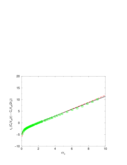
Figure 6: Comparison of the lattice results for the ground state potential between two static ${\bf 3}$ and ${\bf\bar{3}}$ sources and the fit to $V_{eff}$ given by Eq. (47) (solid line), and Eq. (73) (dashed line). Lattice data (boxes) come from Ref. latt1

The new contribution to the gap arising from the $Q{\bar{Q}}G$ cluster contains matrix elements of $H$ evaluated between the BCS vacuum and a tree particle, $Q{\bar{Q}}G$ state or between $Q{\bar{Q}}G$ and $Q{\bar{Q}}$ states. Only $V_{qg}$ and $H_{C}$ contribute to those and they are of order $O(g\sim\langle d(|{\bf k}|)\rangle)$ and $O(g^{3}\sim\langle d^{3}(|{\bf k}|)\rangle)$ respectively. As discussed in Ref. ss7 the later is of a type of a vertex correction and is expected to be a small $O(10-20\%)$ correction to an $O(g)$ contribution from $V_{qg}$. Therefore we will not further included it here (this is also consistent with the ring-rainbow approximation to $V_{eff}$). The final expression for $\delta m_{g}$ also requires $Q{\bar{Q}}G$ wave functions i.e the eigenstates of $H_{0}+H_{C}$ projected onto the $Q{\bar{Q}}G$ states. In this work we do not attempt to solve this eigenvalue problem instead we will approximate the sum over 3-particle intermediate states by,

$$\sum_{n}|n\rangle{1\over{E_{n}-E_{\Omega_{BCS}}}}\langle n|\longrightarrow|\Psi\rangle{1\over{E_{\Psi}-E_{\Omega_{BCS}}}}\langle\Psi|+\sum_{Q{\bar{Q}}G,(E_{Q{\bar{Q}}G}-E_{\Omega_{BCS}})>\Lambda_{F}}|Q{\bar{Q}}G\rangle{1\over{E_{Q{\bar{Q}}G}-E_{\Omega_{BCS}}}}\langle Q{\bar{Q}}G|,$$ (53)

i.e. we approximate the sum over the complete set of eigenstates by a single state with energy smaller then some factorization scale, $\Lambda_{F}$, $E_{\Psi}-E_{\Omega_{BCS}}<\Lambda_{F}$, and a perturbative continuum of states with energy grater then $\Lambda_{F}$. The scale $\Lambda_{F}$ should roughly equal the energy where, due to string breaking the linear confining potential saturates. For the first excited hybrid potential $\Lambda_{F}\mathrel{\hbox to0.0pt{\lower 4.0pt\hbox{\hskip 1.0pt$\sim$}\hss}\raise 1.0pt\hbox{$>$}}1.5\mbox{GeV}$ which corresponds to the distance between color sources, $r=1.15\mbox{ fm}$ Bali . Thus we expect that the size of the momentum space wave function, $\langle Q{\bar{Q}}G|\Psi\rangle$ should be of the order $\beta\sim 1/r=0.2\mbox{GeV}$. As for the spin-orbital momentum dependence of the $Q{\bar{Q}}G$ wave function we shall assume that it corresponds to low values of the orbital angular momenta which are consistent with those of the low lying gluonic excitations in the presence of $Q{\bar{Q}}$ sources. Lattice computation of the $Q{\bar{Q}}$ adiabatic potentials arising from excited gluon configurations indicate that the so called $\Pi_{u}$ potential has lower energy then the $\Pi_{g}$ potential latt1 . These two correspond to gluon configuration with $J^{PC}=1^{+-}$ and $1^{--}$ respectively which is also consistent with the bag model representation of gluonic excitations bag . The $Q{\bar{Q}}G$ wave function coupled with the $J^{PC}=1^{+-}$ gluon quantum numbers would also have the $Q{\bar{Q}}$ pair with the same $J^{PC}=1^{+-}$ quantum numbers (to give the overall $J^{PC}=0^{++}$ of the vacuum) and would be given by

$$\left[Q{\bar{Q}}G\right]^{0} = \left[\left[(L_{Q\bar{Q}}=1)\times(S_{Q\bar{Q}}=0)\right]^{1}\right.$$ (54)

$$\times \left.\left[(L_{G}=1)\times(S_{G}=1)\right]^{1}\right]^{0}.$$

It is easy to check, however, that since $V_{qg}$ is spin dependent this wave function has vanishing overlap with the $V_{qg}|\Omega\rangle$ state. The other possibility is to take $J^{PC}=1^{--}$ configurations for both the glue and the quark-antiquark which give,

$$\left[Q{\bar{Q}}G\right]^{0} = \left[\left[(L_{Q\bar{Q}}=0)\times(S_{Q\bar{Q}}=1)\right]^{1}\right.$$ (55)

$$\times \left.\left[(L_{G}=0)\times(S_{G}=1)\right]^{1}\right]^{0}.$$

and take the spin-orbit wave function in the form of,

$$\langle Q({\bf k}_{Q},\lambda_{Q},i_{Q}),{\bar{Q}}({\bf k}_{\bar{Q}},\lambda_{\bar{Q}},i_{\bar{Q}}),G({\bf k}_{G},\lambda_{G},a)|\Psi\rangle=(2\pi)^{3}\delta({\bf k}_{Q}+{\bf k}_{\bar{Q}}+{\bf k}_{G})U^{{\dagger}}({\bf k}_{Q},\lambda_{Q})\bbox{\alpha}\cdot\bbox{\epsilon}({\bf k}_{G},\lambda_{G})V({\bf k}_{\bar{Q}},\lambda_{\bar{Q}})\Psi({\bf k}_{Q},{\bf k}_{\bar{Q}},{\bf k}_{G}).$$ (56)

The color part of the wave function is given by $T^{a}_{i_{Q},i_{\bar{Q}}}$, and for the orbital wave function we will take a gaussian ansatz,

$$\Psi({\bf k}_{Q},{\bf k}_{\bar{Q}},{\bf k}_{G})=exp(-({\bf k}^{2}_{Q}+{\bf k}^{2}_{\bar{Q}}+{\bf k}^{2}_{G})/\beta^{2}).$$ (57)

The expression for $\delta m_{g}$ is then given by,

$$\delta m_{g}=\delta m_{g}(|{\bf q}|)=\delta m_{g,soft}+\delta m_{g,hard},$$ (58)

with

$$\delta m_{g,soft}=- {{C_{F}}\over{E_{\Psi}-E_{\Omega}}}\int{{d{\bf k}}\over{(2\pi)^{3}}}{{d(|{\bf k}-{\bf q}|)\Psi({\bf k},{\bf q},{\bf k}-{\bf q})/|\Psi|}\over{\sqrt{\omega(|{\bf q}-{\bf k}|)}}}\left[s_{\bf k}c_{\bf q}-I({\bf k},{\bf q})c_{\bf k}s_{\bf q}\right]$$ (59)

$$\times\int{{d{\bf p}}\over{(2\pi)^{3}}}{{d{\bf l}}\over{(2\pi)^{3}}}{{d(|{\bf l}-{\bf p}|)\Psi^{*}({\bf p},{\bf l},{\bf l}-{\bf p})/|\Psi|}\over{\sqrt{\omega(|{\bf l}-{\bf p}|)}}}\left[1+s_{\bf p}s_{\bf l}+I({\bf p},{\bf l})c_{\bf p}c_{\bf l}\right],$$

$$\delta m_{g,hard}=-C_{F}\int{{d{\bf k}}\over{(2\pi)^{3}}}{{d^{2}(|{\bf k}-{\bf q}|)}\over{|{\bf q}-{\bf k}|}}{{\left(1-\Psi_{\Lambda_{F}}({\bf k},{\bf q},{\bf k}-{\bf q})\right)}\over{|{\bf k}|+|{\bf q}|+|{\bf k}-{\bf q}|}}\left[s_{\bf k}c_{\bf q}-I({\bf k},{\bf q})c_{\bf k}s_{\bf q}\right].$$ (60)

Here

$$I({\bf k},{\bf q})\equiv{{(|{\bf k}|^{2}+|{\bf q}|^{2}){\hat{\bf k}}\cdot{\hat{\bf q}}-|{\bf k}||{\bf q}|(1+({\hat{\bf k}}\cdot{\hat{\bf q}})^{2})}\over{({\bf k}-{\bf q})^{2}}},$$ (61)

$$|\Psi|^{2}=\int{{d{\bf p}}\over{(2\pi)^{3}}}{{d{\bf l}}\over{(2\pi)^{3}}}|\Psi({\bf p},{\bf l},{\bf l}-{\bf p})|^{2}\left[1+s_{\bf p}s_{\bf l}+I({\bf p},{\bf l})c_{\bf p}c_{\bf l}\right],$$ (62)

and $\Psi_{\Lambda_{F}}$ given by Eq. (57) with $\beta\to\Lambda_{F}$ so that $1-\Psi_{\Lambda_{F}}$ cuts off hard $Q{\bar{Q}}G$ contribution for energies below $\Lambda_{F}$.

III.1 UV behavior and renormalization

Before analyzing the full gap equation and in particular the effects of $\delta m_{g}$, we shall first discuss the IR and UV behavior in the BCS approximations. The BCS approximation to the chiral gap has been studied earlier for various model approximations to $V_{eff}$. Most of them use an effective potential which is regular at at the origin, e.g a pure linear potential $V_{eff}(r)=br$ chha ; Cotan or a harmonic oscillator, $V_{eff}(r)=kr^{2}$ Lis . For such potentials the gap equation is finite in the high momentum limit and no renormalization is required. This is not the case if potential has the Coulomb component with $V_{eff}(r\to 0)\sim\alpha/r$ and $\alpha$ being either a constant or a running coupling $\alpha\to\alpha(r)\sim 1/\ln(1/r)$. The BCS quark gap for potentials with the Coulomb tail was studied in Ref. AA ; swif and Ref. ss3 . The gap equation used in Ref. AA would be identical to one used here, if $\delta m_{g}$ was set to zero (e.g. the BCS approximation). Instead, in Ref. AA an energy-independent interaction motivated by a transverse gluon exchange was added. In Ref. AA it was argued that, in the chiral limit, the resulting gap equation, could be renormalized by introducing a single counterterm representing the wave function renormalization. Starting from the Coulomb gauge Hamiltonian this would arise if the free quark kinetic energy term was replaced by a renormalized one,

$$\int d{\bf x}{\bar{\psi}}({\bf x})\left[-i\bbox{\alpha}\cdot\bbox{\nabla}\psi({\bf x})\right]$$

$$\to Z(\Lambda)\int d{\bf x}{\bar{\psi}}({\bf x})\left[-i\bbox{\alpha}\cdot\bbox{\nabla}\psi({\bf x})\right]_{\Lambda}$$ (63)

The explicit, UV cutoff-$\Lambda$ dependence regularizing the kinetic operator can be introduced, for example by field smearing, however, the regularization procedure becomes irrelevant once the resulting gap equation is renormalized. The unrenormalized BCS, gap equation (without effects from transverse gluons) is then given by,

$$Z(\Lambda)m(|{\bf q}|)={C_{F}\over 2}\int^{\Lambda}{{d{\bf k}}\over{(2\pi)^{3}}}V_{eff}({\bf k}-{\bf q}){{m({\bf k})}\over{\sqrt{{\bf k}^{2}+m^{2}({\bf k})}}}-{C_{F}\over 2}\int^{\Lambda}{{d{\bf k}}\over{(2\pi)^{3}}}V_{eff}({\bf k}-{\bf q}){\hat{\bf k}}\cdot{\hat{\bf q}}{{|{\bf k}|}\over{|{\bf q}|}}{{m({\bf q})}\over{\sqrt{{\bf k}^{2}+m^{2}({\bf k})}}},$$ (64)

where we have defined the constituent mass, $m(|{\bf k}|)$ by $m(|{\bf k}|)\equiv|{\bf k}|\sin_{\bf k}$. The renormalized equation is obtained by a single subtraction i.e. by fixing the $\Lambda$-independent solution, $m(|{\bf k}|)$ at a specific value of $|{\bf q}|=|{\bf q}_{0}|$. This leads to a ($\Lambda$ and ${\bf q}_{0}$-independent), renormalized gap equation,

$$m(|{\bf q}|)\lim_{\Lambda\to\infty}\left[I_{m}(|{\bf q}_{0}|,\Lambda)-I_{Z}(|{\bf q}_{0}|,\Lambda)\right]=m({\bf q}_{0})\lim_{\Lambda\to\infty}\left[I_{m}(|{\bf q}|,\Lambda)-I_{Z}(|{\bf q}|,\Lambda)\right],$$ (65)

$$I_{m}(|{\bf q}|,\Lambda)\equiv{C_{F}\over 2}\int^{\Lambda}{{d{\bf k}}\over{(2\pi)^{3}}}V_{eff}({\bf k}-{\bf q}){{m({\bf k})}\over{\sqrt{{\bf k}^{2}+m^{2}({\bf k})}}},\;\;I_{Z}(|{\bf q}|,\Lambda)\equiv{C_{F}\over 2}\int^{\Lambda}{{d{\bf k}}\over{(2\pi)^{3}}}V_{eff}({\bf k}-{\bf q}){\hat{\bf k}}\cdot{\hat{\bf q}}{{|{\bf k}|}\over{|{\bf q}|}}{{m(|{\bf q}|)}\over{\sqrt{{\bf k}^{2}+m^{2}({\bf k})}}},$$ (66)

Whenever possible we will also use the notation $I(|{\bf q}|)\equiv I(|{\bf q}|,\infty)$. We will now show that, this equation does not have a well behaved, nontrivial solution vanishing asymptotically in the large momentum limit, as it was assumed, for example in Ref. AA . Before we do that first we need to take care of the possible IR divergences which appear in the integrals when ${\bf k}\to{\bf q}$. In this limit $V_{eff}({\bf k}-{\bf q})$ is highly divergent, reflecting the long range nature of the confining interaction, e.g. $V_{eff}({\bf k}-{\bf q})\propto 1/({\bf k}-{\bf q})^{4}$ for the linear potential. The gap equation, however, is finite due to cancellation of the numerators between $I_{m}$ and $I_{Z}$. To make individual integrals well behaved we can split the IU and UV parts of $V_{eff}$ defining,

$$V^{IR}({\bf k},M)\equiv\theta(M-|{\bf k}|)V_{eff}(|{\bf k}|),$$

$$V^{UV}({\bf k},M)\equiv\theta(|{\bf k}|-M)V_{eff}(|{\bf k}|),$$ (67)

since $V^{IR}({\bf k},M)+V^{UV}({\bf k},M)=V_{eff}({\bf k})$ and gap equation is independent on the parameter $M$ and we will not write it explicitly. The gap equation becomes,

$$m(|{\bf q}|)={1\over{A+B(|{\bf q}|)}}\left[I^{IR}_{m}(|{\bf q}|)-I^{IR}_{Z}(|{\bf q}|)+I^{UV}_{m}(|{\bf q}|)\right],$$ (68)

where

$$A=A(|{\bf q}_{0}|)={{\left[I^{IR}_{m}(|{\bf q}_{0}|)-I^{IR}_{Z}(|{\bf q}_{0}|)+I^{UV}_{m}(|{\bf q}_{0}|)\right]}\over{m(|{\bf q}_{0}|)}},$$ (69)

and

$$B(|{\bf q}|)=B(|{\bf q}|,|{\bf q}_{0}|)={{I_{Z}^{UV}(|{\bf q}|)}\over{m(|{\bf q}|)}}-{{I_{Z}^{UV}(|{\bf q}_{0}|)}\over{m(|{\bf q}_{o}|)}}.$$ (70)

For given ${\bf q}_{0}$, $A$ is a constant and $B$ is a function of ${\bf q}$, and both, $A$ and $B$ are well defined. In $A$ the IR divergences cancel between $I^{IR}_{m}(|{\bf q}_{0}|)$ and $I^{IR}_{Z}(|{\bf q}_{0}|)$, and $I^{UV}_{m}$ is finite if $m(|{\bf q}|)\to 0$ as ${\bf q}\to\infty$. In $B$ each term is IR finite and the UV divergences cancel between the two terms in Eq. (70). It is easy to show that for $|{\bf q}|>>M,|{\bf q}_{0}|$ the function $B(|{\bf q}|)$ , behaves as,

$$B(|{\bf q}|)\to-C_{F}{\alpha\over{3\pi}}\log{\bf q}^{2}$$ (71)

for $V_{eff}(|{\bf k}|)\to 4\pi\alpha/|{\bf k}|^{2}$ as $|{\bf k}|\to\infty$. If $\alpha$ is replaced by a running coupling then $|B(|{\bf q}|)|$ grows with $|{\bf q}|$ like $\log\log{\bf q}^{2}$. From Eq. (68) it thus follows that for some $|{\bf q}|/|{\bf q}_{0}|>>1$, $A+B(|{\bf q}|)$ changes sign and therefore the equation is undefined. This also remains true if an additional transverse potential is added as done in  AA . In this case the the argument of the integrals defining function the $B(|{\bf q}|)$ becomes,

$${\hat{\bf k}}\cdot{\hat{\bf q}}{{|{\bf k}|}\over{|{\bf q}|}}V^{UV}({\bf k}-{\bf q})\to{{|{\bf k}|}\over{|{\bf q}|}} \left[V^{UV}({\bf k}-{\bf q}){\hat{\bf k}}\cdot{\hat{\bf q}}\right.$$

$$\left.+2I({\bf k},{\bf q})V^{UV}_{T}({\bf k}-{\bf q})\right]$$

For $V_{T}({\bf k})=4\pi\alpha/({\bf k}^{2}+const)$ (as used in Ref. AA ) the additional transverse potential does not contribute to the $\log{\bf q}^{2}$ (or $\log\log{\bf q}^{2}$) behavior of $B(|{\bf q}|)$. In our case there would be a similar contribution arising from the hard part of the gluon exchange given by $\delta m_{g,hard}$. At large $|{\bf q}|$ it adds, a positive , $+C_{F}{\alpha\over{12\pi}}\log{\bf q}^{2}$ contribution to $B(|{\bf q}|)$ and therefore does not cause problems on its own but at the same time does not eliminate the singularity from the Coulomb potential since the net effect is such that $B(|{\bf q}|)\to-\infty$ as $|{\bf q}|\to\infty$.

The problems with the renormalized gap equation for the Coulomb potential is illustrated in Figs. 7 and 8. In this test case we simply take

$$V_{eff}({\bf k}) = V^{IR}({\bf k})+V^{UV}({\bf k})$$ (73)

$$= {1\over C_{F}}{{8\pi b}\over{{\bf k}^{4}}}+{{4\pi\alpha}\over{{\bf k}^{2}\log({\bf k}^{2}/m_{g}^{2}+2)^{n}}}$$

For the string tension, $b=0.24\mbox{ GeV}^{2}$, $\alpha=0.1$, and $n=0$ this gives a good fit to the lattice data as shown in Fig. 6.

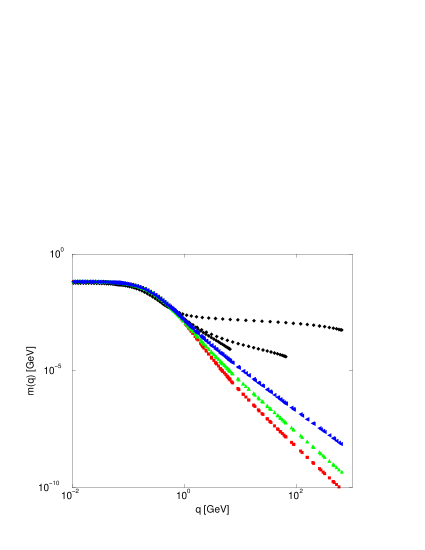
Figure 7: Solution of the gap equation for a potential given by Eq. (73), with $\alpha=1$, and $n=0,1,1/2,3/2$. The three upper lines correspond to $n=0$, the next three to $n=1$, $n=1/2$ and $n=3/2$ respectively

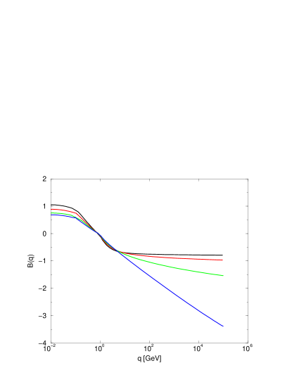
Figure 8: Function $B(|{\bf q}|)$ calculated for the potential as in Fig. 7. The lines (from top to bottom at high $|{\bf q}|$) correspond to $n=3/2$, $n=1/2$, $n=1$ and $n=0$ respectively

In Fig.8 we show the function $B(q)$ calculated from a numerical solution to the gap equation, Eq. (68). Since $V_{eff}$ is already given by a sum of two terms, one dominating in the IR and the other in the UV the components $V^{IR}$ and $V^{UV}$ can be defined as the linear and the Coulomb piece respectively. If $n>1$ there is no renormalization required and the gap equation is given by Eq. (64) with $Z=1$. The $n=3/2$ case corresponds to an approximate analytical solution for $V_{eff}$ discussed in ss7 and is also close to the exact, numerical solution given by Eqs. (47). The solution of the gap equation, $m(q)$ for $n=3/2$ is shown in Fig. 7 by the lowest line (boxes). The function $B(|{\bf q}|)$ corresponding to this case is shown in Fig. 8 by the upper solid line (at large $|{\bf q}|$), which asymptotically approaches $B(|{\bf q}|)\to const-2C_{F}\alpha/(3\pi\log({\bf q}^{2}))$ as $|{\bf q}|\to\infty$. We then take this solution to set the value of $m(|{\bf q}_{0}|=m_{g}=600\mbox{ MeV})$ and solve the renormalized gap equation, Eq. (68) for $n=1$, $n=1/2$ and $n=0$. The asymptotic behavior at large $|{\bf q}|$ of $B(|{\bf q}|)$ for these three cases is given by,

$$B(|{\bf q}|)\to\left\{\begin{array}[]{cc}-C_{F}{\alpha\over{3\pi}}\log\log(|{\bf q}|^{2}),&n=1\\ -2C_{F}{\alpha\over{3\pi}}\log^{1/2}(|{\bf q}|),&n=1/2\\ -C_{F}{\alpha\over{3\pi}}\log(|{\bf q}|),&n=0\end{array}\right.$$ (74)

The corresponding solutions to the gap equation are shown by the five upper lines in Fig. 7. The highest three correspond to $n=0$ case and their splitting indicates that the numerical procedure has not converged into a unique solution. These three solutions correspond to three different cut-offs on the maximum momentum, $|{\bf q}|_{max}=10m_{g},100m_{g}$ and $1000m_{g}$. The other two lines correspond to solutions for $n=1/2$ and $n=1$ respectively. In these two cases the same three values for the momentum cutoffs were used and apparently in both cases a cutoff independent solution has emerged. This is because for $n=1/2$ and $n=1$ $|B(q)|$ grows very slowly and in practice the zero of the denominator in Eq. (68) is not crossed. This test calculation was performed with unphysically large $\alpha=1$. For $\alpha\mathrel{\hbox to0.0pt{\lower 4.0pt\hbox{\hskip 1.0pt$\sim$}\hss}\raise 1.0pt\hbox{$<$}}0.5$ numeral computations, which always have a build in a finite upper momentum cutoff converge for $|{\bf q}|_{max}$ as large as $10^{6}m_{g}$.

It is clear that the problematic UV contributions originate from need for wave function renormalization. This problem has been resolved in Ref. ss3 using an effective Hamiltonian with perturbative $O(g^{2})$ contributions calculated via a similarity transformation Glazek . In that approach, in addition to the Coulomb and transverse gluon contributions to the gap equation, $\delta m_{C}$ and $\delta m_{g,hard}$, there was also a modification of the single particle kinetic. The additional contribution to the gap equation via $\delta m_{0}$ cancels the $\log|{\bf q}|$ term from $B(|{\bf q}|)$ and results in a well defined equation. The disadvantage of that approach however, is that it is restricted to the free rather then BCS basis and so far it has not being generalized beyond perturbation theory.

The resummation of the leading UV contribution to the Faddeev-Popov operator and the Coulomb kernel has the effect of softening the UV behavior (c.f. Eqs. (48), (49)) and at the BCS level leads to a finite gap equation without need for any additional, e.g. wave function renormalization counter-terms. Furthermore the $e^{-S}$ method enables to include effects of transverse gluons with a well defined energy dependence. The large momentum contribution from the $Q{\bar{Q}}G$ cluster, $\delta m_{g,hard}$ still requires renormalization through the wave function counterterm. As discussed above since it leads to $B(|{\bf q}|)$ which is positive at large $|{\bf q}|$ the renormalized gap equation is well behaved.

III.2 Numerical results

We will now discuss the numerical results. These are summarized Fig. 9.

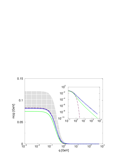
Figure 9: Solution to gap equation. The dashed line is a solution with the IR part of the potential (linear potential) only. The lowest solid line comes from a solution using the full static potential, $\delta m_{C}$. The next higher solid line includes the static potential and the hard gluon, $\delta m_{g,hard}$, contribution from the $Q{\bar{Q}}G$ sector calculated for $\Lambda_{F}=1.5\mbox{ GeV}$. The shaded region corresponds to the full solution with $0.1\mbox{ GeV}\leq\beta\leq 0.4\mbox{ GeV}$, and $1\mbox{ GeV}\leq\Lambda_{F}\leq 2\mbox{ GeV}$

The BCS, potential contribution to the gap equation, $\delta m_{C}$ is split into an IR and UV parts by setting $f({\bf k})=0=d({\bf k})=0$ for $|{\bf k}|>m_{g}$ and $|{\bf k}|<m_{g}$ respectively. For the pure IR potential (dashed line in Fig. 9) the gap function, $m(q)$ is below $100\mbox{ MeV}$ for low $|{\bf q}|<m_{g}$ and it vanishes rapidly (as $1/|{\bf q}|^{4}$) at high $q$. The addition of the UV component of the potential, i.e. the Coulomb tail with the $1/\log(q)^{n},n>1$ UV suppression, does not change much the low momentum behavior of $m(|{\bf q}|)$. It actually decreases $m(0)$ to about $75\mbox{ MeV}$, by it increases the high momentum tail, overall leading to no change in the $\langle{\bar{Q}}Q\rangle$ condensate which stays at about $-(111\mbox{ MeV})^{3}$.

The $\delta m_{g}$ contribution depends on, $\beta$ which sets the size of the soft wave function, $\Lambda_{F}$ which divides between the soft and hard one-gluon intermediate states, and $E_{\Psi}-E_{\Omega}$ which determines the energy of the low gluonic excitations. As discussed earlier it is reasonable to set $\beta\sim 0.2\mbox{ GeV}$ and $\Lambda_{F}\sim 1.5\mbox{ GeV}$. As for the energy of the soft $Q{\bar{Q}}G$ state we take, $E_{\Psi}-E_{\Omega}=m_{g}$ which we expect to be close to the lower bound and would therefore give the upper limit on the $Q{\bar{Q}}G$ contribution. The effect of the hard one-gluon-exchange contribution, defined by $\delta m_{g,hard}$, is to increase $m(q)$ yielding $m(0)\sim 80\mbox{ MeV}$ and enhancing the condensate, $\langle{\bar{Q}}Q\rangle=-(150\mbox{ MeV})^{3}$. The solution to the gap equation including $\delta m_{C}$ and $\delta m_{g,hard}$ is shown by the second to lowest solid line in Fig. 9.

As mentioned above, the gap equation with $\delta m_{g,hard}$ requires renormalization and we have simply set $Z=1$ at $\Lambda=|{\bf q}_{max}|$. Using any of the three values of $|{\bf q}_{max}|$ given previously no effect on the solution could be observed. This is analogous to the test case discussed earlier.

The full effect of the $Q{\bar{Q}}G$ sector, including the soft contribution, parametrized by $\delta m_{g,soft}$ with the factorization scale $\beta$ in the range between $0.1\mbox{ GeV}$ and $0.4\mbox{ GeV}$ and $\Lambda_{F}=1-2\mbox{ GeV}$ is shown by the shaded region. The lower limit corresponds to $\beta=0.1\mbox{ GeV}$ and $\Lambda_{F}=2\mbox{ GeV}$ and yields $\langle{\bar{Q}}Q\rangle=-(140\mbox{ MeV})^{3}$; for the upper limit $\beta=0.4\mbox{ GeV}$, $\Lambda_{F}=1\mbox{ GeV}$ and $\langle{\bar{Q}}Q\rangle=-(190\mbox{ MeV})^{3}$. The addition of the soft gluon intermediate state brings both, the constituent quark mass and the condensate significantly closer to phenomenologically acceptable values.

An alternative simple parameterization of the soft gluon contribution would be to replace it by an effective local operator, by expanding $\delta m_{g,soft}$ in powers of $|{\bf k}|/m_{g}$. The lowest dimension operator has the structure

$$\delta V=-{C\over{m^{2}_{g}}}\int d{\bf x}\left[\psi^{{\dagger}}({\bf x})\alpha^{i}\psi({\bf x})\delta_{T,ij}(\bbox{\nabla}_{{\bf x}})\psi^{{\dagger}}({\bf x})\alpha^{j}\psi({\bf x})\right]_{\beta}$$ (75)

with $C$ being a dimensional constant, $1/m_{g}^{2}$ scale arising from the product of $E_{\Psi}-E_{\Omega_{BCS}}$ and $\omega(0)=m_{g}$, and the operator being related by the factorization scale $\Lambda_{F}$. The appearance of these to scales is quite natural. Since the operator arises through elimination of part of the Fock space the overall scale is given by the excitation energy of the eliminated sectors and the momentum cutoff comes from the spatial extend of the excited state wave function. Such a simple, local approximation of the soft $Q{\bar{Q}}G$ exchange was considered previously in Ref. prl where it was shown that such an operator was indeed relevant to chiral symmetry braking effects, e.g. the condensate and the $\pi-\rho$ mass splitting.

IV Summary

Dynamical breaking of chiral symmetry is the fundamental property of QCD which leads to the constituent representation. In the canonical, Hamiltonian based formulation it arises via the BCS-like pairing between light quark and antiquarks mediated by the attractive Coulomb interaction. However, the extent of chiral symmetry breaking generated this way, as measured by the scalar quark density or as compared to the phenomenological constituent quark model is to small. We have shown that the naive inclusion of the short range part of the $Q{\bar{Q}}$ potential leads to instabilities in the quark gap equations which cannot be renormalized away. In contrast a systematical re-summation of the leading IR and UV corrections to to the bare Coulomb kernel leads to an effective interactions which is consistent with the variational treatment and the gap equation. Using the linked cluster expansion we have estimated the role of three-particle, $Q{\bar{Q}}G$ correlations in the vacuum, and shown that they are indeed important, in particular their low momentum components. Even though we have not used the exact solution describing the soft $Q{\bar{Q}}G$ state our result are expected to be close to the upper bound for the non-BCS contribution to the chiral condensate and are consistent with previous studies.

V Acknowledgment

We would like to thank Bogdan Mihaila for discussion of the $exp(S)$ method. This work was supported by the US Department of Energy under contract DE-FG02-87ER40365.

References

• (1) M.G. Alford, K. Rajagopal, F. Wilczek, Nucl. Phys. B537, 443 (1999). T. Schafer, F. Wilczek, Phys. Rev. D60, 074014 (1999).
• (2) For a review of Dyson-Schwinger results see for example, C.D. Roberts, A.G. Williams, Prog. Part. Nucl. Phys. 33, 477 (1994).
• (3) J.R. Finger, J.E. Mandula, Nucl. Phys. B199, 168 (1982); S.L. Adler, A.C. Davis, Nucl. Phys. B244, 469 (1984); A. Le Yaouanc, et al. Phys. Rev. D31, 137 (1985).
• (4) P.J.de A. Bicudo, J.E.F.T. Ribeiro, Phys. Rev. D42, 1611 (1990), ibid. 1625 (1990), 1635 (1990).
• (5) F.J. Llanes-Estrada, S.R. Cotanch, Nucl. Phys. A697, 303 (2002).
• (6) R. Alkofer, P.A. Amundsen, Nucl. Phys. B306, 305 (1988).
• (7) P. Maris, C.D. Roberts, Phys. Rev. C56, 3369 (1997); P. Maris, P.C. Tandy, Phys. Rev. C62, 055204 (2000).
• (8) A.P. Szczepaniak, E.S. Swanson, C.-R. Ji, S.R. Cotanch, Phys. Rev. Lett. 76, 2011 (1996); A.P. Szczepaniak, E.S. Swanson, Phys. Rev. D55, 3987 (1997).
• (9) A.P. Szczepaniak, E.S. Swanson, Phys. Rev. D55, 1578 (1997).
• (10) D. Zwanziger, Nucl. Phys. B518, 237 (1998); A. Cucchieri, D. Zwanziger, Phys. Rev. Lett. 78, 3814 (1997).
• (11) A.P. Szczepaniak, E.S. Swanson, Phys. Rev. D65, 025012 (2002).
• (12) K.J. Juge, J. Kuti, C.J. Morningstar, Nucl. Phys. Proc. Suppl. 63, 326 (1998).
• (13) N.H. Christ, T.D. Lee, Phys. Rev. D22, 939 (1980).
• (14) A.R. Swift, Phys. Rev. D38, 668 (1988).
• (15) H. Kümmel, K.H. Lührmann, J.G. Zabolitzky, Phys. Rep. 36, 1 (1978).
• (16) J.-P. Blaizot, G. Ripka, Quantum Theory of finite Systems, (MIT Press, 1986).
• (17) G.S. Bali e-Print Archive: hep-ph/0010032; G.S. Bali et al. (SESAM Collab.), Phys. Rev. D62, 054503 (2000).
• (18) T. Barnes, F.E. Close, F. de Viron, J. Weyers, Nucl. Phys. B224, 241 (1983); K.J. Juge, J. Kuti, C.J. Morningstar, Nucl. Phys. Proc. Suppl. 63, 543 (1998).
• (19) K.G. Wilson, T.S. Walhout, A. Harindranath, W.-M. Zhang, R.J. Perry, S.D. Glazek, Phys. Rev. D49, 6720 (1994).
• (20) A.P. Szczepaniak, E.S. Swanson, Phys. Rev. Lett., 87, 072001 (2001).