Special relativity constraints on the effective constituent theory of hybrids

Abstract

We consider a simplified constituent model for relativistic strong-interaction decays of hybrid mesons. The model is constructed using rules of renormalization group procedure for effective particles in light-front quantum field theory, which enables us to introduce low-energy phenomenological parameters. Boost covariance is kinematical and special relativity constraints are reduced to the requirements of rotational symmetry. For a hybrid meson decaying into two mesons through dissociation of a constituent gluon into a quark-anti-quark pair, the simplified constituent model leads to a rotationally symmetric decay amplitude if the hybrid meson state is made of a constituent gluon and a quark-anti-quark pair of size several times smaller than the distance between the gluon and the pair, as if the pair originated from one gluon in a gluonium state in the same effective theory.

I Introduction

Hybrid mesons, in particular those with exotic quantum numbers, will play important role in the phenomenology of confinement and studies of low energy gluons. For example, decay patterns of gluonic excitations in hybrid mesons are expected to be quite different from those that characterize ordinary meson resonances. It is predicted that exotic meson decays are dominated by the so-called “S+P” channels that contain pairs of mesons, one with the valence quark-anti-quark pair in the $S$-wave relative motion, and the other with a pair in a $P$-wave, e.g., $\pi b_{1}$, $\pi f_{1}$, or $\pi a_{1}$ isgur . In contrast, non-exotic meson decays are dominated by “S+S” channels, such as $\pi\pi$, $\rho\rho$, $K{\bar{K}}$, etc. These predictions are based on a simple, non-relativistic constituent-quark picture. However, the lightest exotic mesons are expected to be as heavy as $1.6-2$ GeV and their decays will produce mesons that move relativistically. Therefore, this article addresses the issue of constraints that special relativity imposes on the constituent picture of such decays. The other basic requirement satisfied by the relativistic approach developed here is that in principle it is derivable from quantum field theory in agreement with rules of renormalization group for low energy parameters in the constituent Hamiltonians.

In order to analyze data from experiments where photons are absorbed on a hadronic target and produce intermediate hadronic states with masses on the order of 1.5-2.5 GeV, which subsequently decay into mesons $\pi$, $\rho$, or $b$, one must construct a viable picture of strongly interacting bound states. These states, especially $\pi$-mesons, move with velocities comparable to the speed of light, and the whole photo-production and decay process cannot be described using wave functions for hadrons at rest, or in slow motion. At the same time, the principles of quantum field theory have to be obeyed precisely if one demands a clear connection between a phenomenological constituent picture of the process and QCD. Lessons from QED are of great value but QCD interactions are much stronger and pose additional problems with non-perturbative and relativistic effects, which QED is not telling us how to solve beyond Feynman’s perturbation theory.

So far, theoretical insights into the exotic mesons structure are provided by lattice simulations lat1 , and Coulomb-gauge QCD CG , in addition to model studies PP1 ; PP2 . It follows from these studies that the lowest mass and spin exotic mesons are most probably dominated by a constituent gluon coupled to a constituent quark-anti-quark pair. In a more complete picture, one would like the exotic candidate states to be obtainable, at least in principle, from a precisely defined relativistic Hamiltonian for QCD. The decay process should be described by the same Hamiltonian. To satisfy these requirements, one would have to derive the effective constituent particles from quantum field theory. The derivation would have to include description of the constituents’ spin and angular momenta, and how rotating and boosting of bound states to high velocities is accomplished. Such comprehensive relativistic constituent picture is not yet established in QCD and hadronic constituents are far from being understood as well as the non-relativistic constituents of atoms are in QED. However, there exist reasonable theoretical grounds for hope that the required relativistic description of effective quarks and gluons can be found using renormalized light-front (LF) QCD Hamiltonians in $A^{+}=0$ gauge. The reasons for the hope go beyond the pioneering works of Lepage and Brodsky LB and Wilson et al. W6 , and include results that suggest that the effective constituents are derivable in a perturbative renormalization group calculus for the corresponding creation and annihilation operators GQCD . The same calculus is also suggested to be able to produce all generators of the Poincaré algebra in the form ready to use in the effective-particle Fock-space basis SGTM . If these generators were available, the desired construction of hadrons, including exotic hybrid states and fast moving mesons, could be carried out precisely enough to make specific predictions for partial waves branching ratios in decay amplitudes, and the QCD constituent theory of hybrids could be put to definite tests.

The LF approach is a potential alternative to the standard form of Hamiltonian dynamics, where states evolve in usual time. There, rotational symmetry is kinematical, but one needs to worry about boosting the constituent wave functions for the fast moving bound states and their constituents RQM . Nevertheless, much progress has been achieved in building the constituent representation in the usual Coulomb-gauge quantization in the rest frame CG ; CG2 . The connection between bare field quanta and quasi-particles, corresponding to a constituent basis, was obtained and related to spontaneous chiral symmetry breaking. Furthermore, in the gluonic sector, the Coulomb-gauge canonical quantization reproduces the the lattice gauge theory results for the spectrum of the low-lying gluon modes, e.g., glueballs, and the excited heavy-quark adiabatic potential lat1 . Still, the Lorentz boost covariance of observables in the instant formulation in Minkowski space is not yet established, and poses problems analogous to rotational symmetry issue in the boost invariant LF scheme. Both are major theoretical challenges. Here, we will concentrate on the rotational symmetry in the LF description of hadrons in terms of their constituents.

Note, however, that the LF QCD path is not sufficiently developed for immediate identification of all important features of the effective constituent dynamics in hadronic processes. The theory requires initial guidance from phenomenological analysis to begin scanning through and cataloging of the infinite set of potentially relevant operators that are allowed to appear in the effective QCD Hamiltonian. In view of the magnitude of the task, before one dives into the full complexity of LF QCD, one should first find out if rotational symmetry of observables has any chance to be obtained in the boost-invariant picture of hadronic states made of a small number of effective-particle Fock-components. The common belief is that a physically adequate relativistic scheme cannot be achieved using a small number of degrees of freedom. The structural integrity requirement for the effective-particle LF-scheme thus implies that the rotational symmetry condition should be possible to satisfy with some natural easiness, visible already in the most elementary versions of the scheme. Therefore, the question of how hard it is to build a rotationally symmetric model of a hybrid decay amplitude with a minimal number of constituents needs to be answered before a search for approximate solutions to quantum field theory in terms of effective constituents is pursued on a larger scale. Here, we report results of the feasibility test for this scheme, which were obtained with all possible simplifications one could afford preserving only the most basic and universal constraints of special relativity, quantum field theory, and renormalization group for effective particles. All details beyond the core features are removed for transparency of the bottom-line structure.

In principle, the dynamics of hadronic constituents is determined by the effective-particle Hamiltonian. Once such a Hamiltonian is constructed, one can attempt to solve the corresponding Schrödinger equation and calculate the hybrid decay in terms of the effective-particle interactions and states. The basic study reported here is carried out instead by simplifying the initial canonical Hamiltonian theory to the ultimate minimum, deriving the effective theory in a crudest lowest-order approximation, and using model wave functions typical for phenomenology instead of self-consistent solutions of the currently unknown effective theory. Thus, in practice, we calculate a transition amplitude for a hand-made one three-effective-particle bound state to decay into two hand-made two-effective-particle bound states, and we check if the result has any chance to respect rotational symmetry.

This paper is organized as follows. Section II describes the key elements of the constituent scheme used here. It is assumed that the interaction responsible for the hybrid decay comes from an effective Hamiltonian obtained from a local quantum field theory via renormalization group procedure for effective particles. Section III describes details of the model states of hybrids and mesons, and the transition amplitude for the hybrid decay into the two mesons. Wave functions of the incoming and outgoing states are written down on the basis of well-known phenomenology, but without solving the effective Schrödinger equation. Nevertheless, we allow a whole set of free parameters in them in order to cover a large range of possible structures and find out if it is possible (and if so, then for what choices of the parameters) to obtain rotationally symmetric results. Numerical results from our review of the angle dependence of the decay amplitude are discussed in Section IV. Section V draws conclusions that concern phenomenological studies of hybrid production and decay processes and can be directly useful in comparing data from future experiments with a theory of effective particles in QCD.

II Key elements

In order to remove the basic issues of spin, gauge invariance, current conservation, and effective mass of gluons, from the preliminary constituent study, and to focus on general quantum mechanical and relativistic features of the effective particle dynamics, one can assume that gluons are scalars. In order to do better than that at the current level of understanding of the effective gluon dynamics, one would have to clearly answer questions concerning Lorentz transformation properties of massive gluons with spin one and only two, instead of three polarization states. Since the answer is lacking, the issue is avoided by the arbitrary simplification.

With the gluon spin issue removed, the scalar-iso-scalar bare gluon can still be coupled to an iso-doublet of bare quarks like in a Yukawa theory. Thus, the bare “gluon” has only color as in QCD, while the coupling to bare quarks is given by the term

$${\cal H}_{int}=g\bar{\psi}A^{a}t^{a}\psi\quad,$$ (1)

where the gluon field does not have a vector index. In this model, the first order solution of renormalization group equations for the effective gluon coupling to effective quarks produces the term SGMW

$$gf_{\lambda}\bar{\psi}_{\lambda}A^{a}_{\lambda}t^{a}\psi_{\lambda}\quad,$$ (2)

where $\lambda$ denotes the renormalization group parameter. It has dimension of mass. Its scale can be intuitively associated with the transverse size of the effective particles and $f_{\lambda}$ denotes the vertex form factor. The width of the form factor in momentum space is given by $\lambda$. The effective particles that can be considered appropriate for the lowest Fock-sector picture of hadrons are expected to emerge when $\lambda$ is lowered by solving similarity renormalization group equations for Hamiltonians down to the scale of hadronic masses, possibly to the values on the order of 1 to several GeV, when one aims at description of a hybrid meson in terms of a quark-anti-quark pair and a gluon.

The factor $g$ stands for the vertex strength function $v_{\lambda}$ that at some value of the momentum transfer defines a running coupling constant in the Hamiltonian GQCD , denoted by $g_{\lambda}$. In the first order solution of renormalization group equations, $v_{\lambda}$ equals $g$. In higher orders, this coupling would be replaced by $g_{\lambda}$ and the latter could be quite large in QCD when $\lambda$ is of the order of hadronic masses. However, the large coupling is not sufficient to make the effective interaction strong enough to wash out the constituent picture of the individual hadrons, as it would happen in a local canonical theory with equally large coupling constants. The reason is that the vertex form factor cuts off interactions with momentum transfers larger than $\lambda$, and they are effectively much weaker, like in nuclear physics. Therefore, the bound state picture with a small number of massive constituents may be still valid when $\lambda$ is small. Eq.(2) provides also a potentially valid structure for at least a part of the interaction responsible for the decay of a model constituent “gluon” into the effective quark and anti-quark pair. The “gluon” decay factor in the model hybrid decay amplitude can thus be assumed to be given by the product of the form

$$gf_{\lambda}(12)\bar{u}_{1}v_{2}\quad,$$ (3)

times the corresponding color factor $\chi^{\dagger}_{c1}t^{a}\chi_{c2}$. One may simplify the constituent picture even farther for the purpose of this study, and replace fermionic quarks by scalars, too. The required interaction, analogous to (1), would be

$$H_{int}=g\xi^{\dagger}A^{a}t^{a}\xi\quad,$$ (4)

where $\xi$ is the colored scalar quark field, and the interaction factor in the decay, analogous to (3), would reduce to

$$gf_{\lambda}(12)\quad,$$ (5)

the color factor being the same as for fermions. Both cases of spin-1/2 and spin-0 constituents are described in this paper to show that the features they display are general and independent of spin. This is one of the reasons why one can expect them to occur also in the future QCD calculations.

Even a modest attempt at a self-consistent dynamical solution of a relativistic field-theoretic model with coupled three-body and two-body bound states is a large project. Our goal here is not to carry out such project but to find out if the proposed scheme has a chance to produce rotationally symmetric decay amplitude. Moreover, even if a constituent picture may satisfy the special relativity constraints, the correct effective QCD theory is not known yet. In order to see how strong the relativity constraints are, the simplest thing to do is to assume that the outgoing mesons and decaying hybrid are both scalars and iso-scalars, and to write down candidates for their wave functions in the effective constituent basis with a priori unknown parameters that are constrained only by reasonable guesses about their natural sizes. If the rotational symmetry constraints cannot be satisfied within this class of models, it is unlikely that a simple constituent model can ever be built in more complex cases with additional dynamical constraints. Thus, for example, we assume here only that a meson has a Gaussian momentum-space relative-motion wave function with width $\beta$. Its spatial radius is of the order of $1/\beta$ (if $\beta$ is not too large in comparison to the constituent masses and the meson mass since relativistic effects may change connection between $\beta$ and the radius making it less constraining KS ). Thus, in the first approximation, a meson of size 0.5 fm is expected to have $\beta\sim 0.4$ GeV. In the theory of scalar effective constituents, no further considerations are required for constructing plausible test candidates for the relative-motion wave functions, and none is incorporated here.

In the more complex case of fermions, one has to decide in addition how to combine spins in the wave functions for effective constituents. Solutions of effective fermion theory are also not known, and one is currently in the similar position here as in trying to guess hadronic wave functions in phenomenological studies in the nonrelativistic quark model Isgur1 . The simplest standard phenomenological procedure is to assume that the spin wave functions for the lowest effective Fock components are the same as for multiplets of Poincaré group representations for free particles, i.e., products of free Dirac spinors in the case of fermions. For scalar (colorless) hadrons made of $q\bar{q}$ pairs, one would use spin factors of the form $\bar{u}_{1}v_{2}$ (the color factor would be $\chi^{\dagger}_{c1}\chi_{c2}$). The spin amplitudes would be multiplied by the relative momentum-dependent factors that would be of similar form as in the scalar case.

The relative-motion scalar wave-function factors represent binding and allow for shifting the total free energy of the intermediate constituent particles away from that of the energy shell value for the hybrid itself and the outgoing meson products. This shift in energy is associated with conservation of the total three-momentum of all particles. In the LF Hamiltonian dynamics, however, the conserved momenta are not the same as in the dynamics developed in Minkowski’s time. Instead, the conserved momentum components (in conventional notation) are $p^{+}=p^{0}+p^{3}$ and $p^{\perp}$, where $\perp=$ 1, or 2. The role of energy is played by $p^{-}$, which for a free particle of mass $m$ would be $p^{-}=(p^{\perp\,2}+m^{2})/p^{+}$.

The key Lorentz invariance test, associated with the complicated dynamics of rotations in the LF coordinates, is reduced to the question if the off-shell energy shift in the direction of $p^{-}$ does, or does not introduce significant artificial angular asymmetries in the model hybrid decay amplitude. For example, can one avoid a sizable dependence of the amplitude on the angles at which the scalar mesons fly away from the scalar hybrid decay event in the hybrid center of mass system of reference? If such angle dependence would unavoidably develop in the simplest scalar or fermion model to intolerable degree, one would have to doubt that the simple constituent picture could suddenly become valid in QCD. If rotational symmetry can be approximately obtained, one could hope that proceeding along the line outlined in Refs. SGTM and SGMW , corrections can be refined and eventually a precise theory obtained.

It was mentioned earlier in Section I that when seeking Hamiltonian dynamics for effective particles in the instant (or usual time) form, one would have to make tests of boost invariance. One could then say that the deviations from rotational symmetry one may observe in a LF approach provide a measure of how large deviations from boost covariance can be expected in models based on the standard form of field-theoretic constituent dynamics, even if they respect rotational symmetry in some frame of reference exactly.

III The model

The $q{\bar{q}}$-meson and $q{\bar{q}}g$-hybrid wave functions are constructed by analogy with decomposing a product of representations of the Lorentz group for two and three noninteracting particles into irreducible representations defined by their invariant mass and $J^{PC}$ quantum numbers. The free-particle on-shell invariant mass constraint corresponds to a state with a wave function proportional to a $\delta$-function in the invariant mass. In the model, mesons are constructed by superposing such states in the form of an integral with a Gaussian wave-function factor that depends on the invariant mass Lor , or, equivalently, on the length of the corresponding center-off-mass momenta. Before a theoretically sound, realistic constituent Hamiltonian in QCD is identified, such approach to building models of the non-perturbative hadron structure is quite common, e.g., in the constituent models, or, with some variation, in QCD sum rules.

III.1 $q{\bar{q}}$ Mesons

The two-constituent (or $q{\bar{q}}$) meson state is written as

$$|p\rangle=\sum_{12}\int[12]\,\,p^{+}\tilde{\delta}(1+2-p)\Psi_{J^{PC}}(1,2)\,\,b^{\dagger}_{1}d^{\dagger}_{2}|0\rangle\;,$$ (6)

where $1$ and $2$ collectively represent all quantum numbers of the quark and anti-quark, i.e. the LF 3-momenta, $p^{+}$, $p^{\perp}$, spins, and charges, respectively. The (free) Lorentz-invariant integration measure, denoted in Eq. (6) and similarly later by $[12]$, is given by

$${dk^{+}_{1}d^{2}k^{\perp}_{1}\over 16\pi^{3}k^{+}_{1}}{dk^{+}_{2}d^{2}k^{\perp}_{2}\over 16\pi^{3}k^{+}_{2}}={dx_{12}d^{2}k^{\perp}_{12}\over 16\pi^{3}x_{12}(1-x_{12})}{dP^{+}_{12}dP_{12}^{\perp}\over 16\pi^{3}P^{+}_{12}}\,,$$ (7)

where for all three components of the 3-momenta, $P_{12}=k_{1}+k_{2}$, $k_{12}=(1-x_{12})k_{1}-x_{12}k_{2}$, and $x_{12}=k^{+}_{1}/P^{+}_{12}$. Also, $\tilde{\delta}(1+2-p)=16\pi^{3}\delta(P^{+}_{12}-p^{+})\delta^{2}(P^{\perp}_{12}-p^{\perp})$. Due to the kinematical nature of Lorentz boost invariance of the LF scheme, even in the fully interacting theory, the coordinates $P^{+,\perp}_{12}$, $x_{12}$, and $k^{\perp}_{12}$, enable one to separate the relative constituent motion from the bound-state center-of-mass motion. In general, in the $n$-particle case, the relative-motion variables that are independent of the bound-state momentum $p$ are given by ($i=1,\cdots,n$)

$$x_{i}\equiv k^{+}_{i}/p^{+},\;\;k^{\perp}_{i}\equiv k^{\perp}_{i}-x_{i}p^{\perp}\,.$$ (8)

For given quantum numbers $J^{PC}$, the wave function $\Psi_{J^{PC}}(1,2)$ is a product of color, flavor, spin, and orbital parts, and can be written as,

$$\Psi_{J^{PC}}(1,2)=\chi^{\dagger}_{c_{1}}C\chi_{c_{2}}\,\,\chi^{\dagger}_{i_{1}}I\chi_{i_{2}}\,\,\chi^{\dagger}_{s_{1}}S(1,2)\chi_{s_{2}}\,\,\psi_{p}(1,2)\,\,,$$ (9)

with $C=1/\sqrt{3}$ for a color singlet, $I=1/\sqrt{2}$ for an iso-scalar, and $I=\vec{\tau}/\sqrt{2}$ for an iso-vector meson. Since iso-spin is irrelevant for our studies of Lorentz symmetry, further explicit consideration of the model is limited to iso-scalar meson states.

The model spin-wave function $\chi^{{\dagger}}S(1,2)\chi$ originates from the product of free Dirac spinors. In this analysis, however, we do not perform a detailed phenomenological study for all exotic meson decay channels and we are not concerned about particulars of the spin-orbit couplings for the corresponding $q\bar{q}$ states. For example, $J^{PC}=0^{-+}$, $q{\bar{q}}$-meson wave function could involve the product ${\bar{u}}_{1}\gamma_{5}v_{2}$ as the spin factor. However, for the critical check if the rotational symmetry can be obtained at all, we do not need to insist on constructing states with arbitrary $J^{PC}$ quantum numbers for the mesons in question (here, two, or three, non-interacting constituents). Instead, we choose a simplest scalar form ${\bar{u}}_{1}v_{2}$ for all decay products. This ansatz already introduces some spin-orbit structure and we can use it to check the sensitivity of our numerical estimates to the presence of relativistic spin-orbit couplings. Note that in the calculation of decay amplitude the spins of the constituents are summed over and it does not matter what spin basis on chooses. Nevertheless, the natural choice in the LF scheme is to use Melosh spinors,

$$u(k\sigma)=B(k,m_{q})u(0\sigma)\;\;,$$

$$v(k\sigma)=B(k,m_{q})v(0\sigma)\;\;,$$

$$v(k\sigma)=Cu^{*}(k\sigma)=i\gamma^{2}u^{*}(k\sigma)\;\;,$$ (10)

with

$$B(k,m)={1\over\sqrt{k^{+}m}}[\Lambda_{+}k^{+}+\Lambda_{-}(m+k^{\perp}\alpha^{\perp})],$$ (11)

which represents a LF-symmetry boost from rest to momentum $k$ for a free particle of mass $m$, using conventions $\Lambda_{\pm}={1\over 2}\gamma_{0}\gamma^{\pm}$, $u^{T}(0\sigma)=\sqrt{2m_{q}}[\chi^{T}_{\sigma},0]$, $v^{T}(0\sigma)=\sqrt{2m_{q}}[0,\xi^{T}_{-\sigma}]$, and $\xi_{-\sigma}=-i\sigma^{2}\chi_{\sigma}$. Adopting these conventions, one obtains

$$S(1,2)={1\over\sqrt{x_{12}(1-x_{12})}}\left[m_{q}(2x_{12}-1)\sigma^{3}+k_{12}^{\perp}\sigma^{\perp}\right]i\sigma^{2}.$$ (12)

The orbital wave function $\psi_{p}(1,2)\equiv\psi_{p}(\vec{k}_{12})$ is chosen to be Gaussian, i.e.,

$$\psi_{p}(\vec{k}_{12})=N_{p}\,\,\sqrt{{\cal M}_{12}\over 2m_{q}}\,\,\sqrt{1\over 2({\cal M}_{12}^{2}-4m_{q}^{2})}\,\,\exp{\left[{-{\vec{k}}_{12}^{\,2}\over 2\beta_{p}^{2}}\right]}$$ (13)

where the 3-vector $\vec{k}_{12}$ has the $\perp$ components equal to $k_{12}$ and the $z$-component is defined by DN ,

$${\cal M}^{2}_{12}=(k_{1}+k_{2})^{2}={m^{2}_{q}+k_{12}^{\perp\,2}\over x_{12}(1-x_{12})}=4({\vec{k}}^{\,2}_{12}+m^{2}_{q})\;,$$ (14)

so that $k^{3}_{12}=(x_{12}-1/2){\cal M}_{12}$. Note that the subscript $p$ in $\psi_{p}(\vec{k}_{12})$ is not supposed to mean that $\psi_{p}(\vec{k}_{12})$ depends on the bound state momentum $p$, but rather that the wave function corresponds to the meson with quantum numbers collectively denoted by $p$, and the notational simplification should not be a source of confusion when we consider three mesons simultaneously.

In terms of the 3-vector $\vec{k}_{12}$, the integration measure over the relative motion of the two constituents, is given by

$${dx_{12}d^{2}k^{\perp}_{12}\over 16\pi^{3}x_{12}(1-x_{12})}={4d^{3}\vec{k}_{12}\over 16\pi^{3}{\cal M}_{12}}\;.$$ (15)

The normalization condition $\langle p|p^{\prime}\rangle=p^{+}\tilde{\delta}(p-p^{\prime})$, implies,

$${1\over 16\pi^{3}}\int{4d^{3}k_{12}\over{\cal M}_{12}}2({\cal M}_{12}^{2}-4m_{q}^{2})|\psi_{p}(1,2)|^{2}=1\;,$$ (16)

and

$$N_{p}={2\pi^{3/4}\over\beta_{p}}\sqrt{2m_{q}\over\beta_{p}}\;.$$ (17)

When we consider scalar constituents, the spin factor $2({\cal M}_{12}^{2}-4m_{q}^{2})$ is absent and the second square-root factor in Eq. (13) is removed, so that the normalization constant remains the same.

III.2 Hybrid Meson

The construction of the hybrid meson state is analogous.

$$|h\rangle=\sum_{123}\int[123]\,h^{+}\tilde{\delta}(1+2+3-h)\Psi_{J^{PC}}(1,2,3)\,b^{\dagger}_{1}d^{\dagger}_{2}a^{\dagger}_{3}|0\rangle,$$ (18)

where the color, flavor, spin, and orbital wave-function factors are given by

$$\Psi_{J^{PC}}(1,2,3) = \,\,\chi^{\dagger}_{c_{1}}C_{h}^{c_{3}}\chi_{c_{2}}\,\,\chi^{\dagger}_{i_{1}}I_{h}\chi_{i_{2}}\,\,\chi^{\dagger}_{s_{1}}S_{h}(1,2)\chi_{s_{2}}$$ (19)

$$\times \psi_{h}(1,2,3)\;,$$

with $C^{c_{3}}_{h}=t^{c_{3}}/2$, $I_{h}=1/\sqrt{2}$, and the quark-anti-quark spin wave function is again of the from ${\bar{u}}_{1}v_{2}$, so that

$$S_{h}(1,2)={1-x_{3}\over\sqrt{x_{1}x_{2}}}\left[m_{q}{x_{1}-x_{2}\over 1-x_{3}}\sigma^{3}+k_{q}^{\perp}\sigma^{\perp}\right]i\sigma^{2}.$$ (20)

The kinematical momentum variables satisfy Eq. (8) with $p^{+},p^{\perp}$ replaced with the hybrid LF-3-momentum, $h$. Similarly, the 3-particle integration measure is given by,

$$\prod_{i=1}^{3}{{dk^{+}_{i}d^{2}k^{\perp}_{i}}\over{16\pi^{3}k^{+}_{i}}}={4d^{3}k_{q}\over 16\pi^{3}{\cal M}_{q}}{d^{3}k_{g}{\cal M}_{qg}\over 16\pi^{3}\sqrt{m_{g}^{2}+k_{g}^{2}}\,\sqrt{{\cal M}_{q}^{2}+k_{g}^{2}}}\;,$$ (21)

where the relative momentum 3-vectors ${\vec{k}}_{q}=(k^{\perp}_{q},k^{3}_{q})$ and ${\vec{k}}_{g}=(k^{\perp}_{g},k^{3}_{g})$, are defined by

$$k^{\perp}_{q}=(x_{2}k_{\perp 1}-x_{1}k_{\perp 2})/(1-x_{3})\;,$$

$$k^{3}_{q}=\left({x_{1}\over 1-x_{3}}-{1\over 2}\right){\cal M}_{q}\;,$$ (22)

and

$$k^{\perp}_{g}=(1-x_{3})k^{\perp}_{3}-x_{3}(k^{\perp}_{1}+k^{\perp}_{2})\;,$$

$$k^{3}_{g}={x_{3}^{2}({\cal M}^{2}_{q}+k^{\perp\,2}_{g})-(1-x_{3})^{2}(m^{2}_{g}+k^{\perp\,2}_{g})\over 2x_{3}(1-x_{3}){\cal M}_{qg}}\;.$$ (23)

${\cal M}_{q}$ and ${\cal M}_{qg}$ are the quark-anti-quark and quark-anti-quark-gluon invariant masses,

$${\cal M}^{2}_{q}=(k_{1}+k_{2})^{2}=(1-x_{3})^{2}{m^{2}_{q}+k_{q}^{\perp\,2}\over x_{1}x_{2}}\;,$$ (24)

$${\cal M}^{2}_{qg} = (k_{1}+k_{2}+k_{3})^{2}$$ (25)

$$= {m_{q}^{2}+k_{1}^{\perp\,2}\over x_{1}}+{m_{q}^{2}+k_{2}^{\perp\,2}\over x_{2}}+{m_{g}^{2}+k_{3}^{\perp\,2}\over x_{3}}-h^{\perp\,2}$$

$$= {{\cal M}_{q}^{2}+k_{g}^{\perp\,2}\over 1-x_{3}}+{m_{g}^{2}+k_{g}^{\perp\,2}\over x_{3}}\;.$$

In terms of the relative momenta, the 3-particle orbital wave function $\psi_{h}(1,2,3)\equiv\psi_{h}(\vec{k}_{q},\vec{k}_{g})$ is assumed to be

$$\psi_{h}(\vec{k}_{q},\vec{k}_{g}) = N_{h}\,\,\sqrt{{\cal M}_{q}\over 2m_{q}}\,\,\sqrt{2m_{q}+m_{g}\over{\cal M}_{qg}}$$ (26)

$$\times \,\,\sqrt{\sqrt{m_{g}^{2}+{\vec{k}}^{\,2}_{g}}\over m_{g}}\,\,\sqrt{\sqrt{{\cal M}_{q}^{2}+{\vec{k}}^{\,2}_{g}}\over 2m_{q}}\,\,{1\over\sqrt{8{\vec{k}}_{q}^{\,2}}}$$

$$\times \,\,\exp{\left[{-{\vec{k}}_{q}^{\,2}\over 2\beta_{hq}^{2}}\right]}\,\,\exp{\left[{-{\vec{k}}_{g}^{\,2}\over 2\beta_{hg}^{2}}\right]}\;.$$

Its structure follows from the requirement that it is a product of two Gaussian functions of the momenta $\vec{k}_{q}$ and $\vec{k}_{g}$, with additional factors chosen so that the wave function normalization condition has a nonrelativistic appearance of a six-dimensional integral over the momenta. In the normalization condition $\langle h|h^{\prime}\rangle=h^{+}\tilde{\delta}(h-h^{\prime})$, fermion spinors introduce a factor, which is compensated by the factor $(8{\vec{k}}_{q}^{\,2})^{-1/2}$ in the wave function. This factor is dropped when we consider scalar constituents. So, in both cases of the fermion and scalar constituents the normalization constant is the same and equals

$$N_{h}={2\pi^{3/4}\over\beta_{hq}}\sqrt{2m_{q}\over\beta_{hq}}\,\,{2\pi^{3/4}\over\beta_{hg}}\sqrt{{8m_{q}m_{g}\over 2m_{q}+m_{g}}\,{1\over\beta_{hg}}}\;.$$ (27)

III.3 Decay

The constituent-gluon decay into a constituent quark-anti-quark pair is assumed to be driven by the Hamiltonian interaction term obtained from first-order solution to the renormalization group equations for effective particle Hamiltonians in quantum field theory. In QCD, the decay amplitude of a hybrid meson into two mesons, calculated in first order in this interaction term, has the form

$$\langle pb|H_{I\,QCD\,\lambda}|h\rangle=\tilde{\delta}(p+b-h)\,\,{\cal A}(p,b,h)\quad,$$ (28)

where the interaction term is given by GQCD

$$H_{I\,QCD\,\lambda}=\sum_{123}\int[123]\,\,\tilde{\delta}(1+2-3)\,\,g\,\,f_{\lambda}(1,2,3)$$

$$\,\,\chi^{\dagger}_{c_{1}}t^{c_{3}}\chi_{c_{2}}\,\,\chi^{\dagger}_{i_{1}}\chi_{i_{2}}\,\,\chi^{\dagger}_{s_{1}}S_{QCD}(1,2,3)\chi_{s_{2}}\,\,b_{1}^{\dagger}d_{2}^{\dagger}a_{3},$$ (29)

The spin-factor $\chi^{\dagger}_{s_{1}}S_{QCD}(1,2,3)\chi_{s_{2}}$ equals $\bar{u}_{1}\not\!\varepsilon_{3}v_{2}$ and $\varepsilon_{3}$ denotes the constituent-gluon polarization four-vector. The form factor $f_{\lambda}$ is given by

$$f_{\lambda}(1,2,3)=f_{\lambda}({\cal M}^{2}_{q}-m^{2}_{g0})=\exp{\left[-{\cal M}^{4}_{q}/\lambda^{4}\right]}\;,$$ (30)

since the effective gluon mass $m_{g0}$ is zero in the first-order $H_{QCD\,\lambda}$.

In our elementary study of the Poincaré symmetry constraints on the constituent picture, the spin factor $\chi^{\dagger}_{s_{1}}S_{QCD}(1,2,3)\chi_{s_{2}}$ is replaced by $\bar{u}_{1}v_{2}$, which one would obtain in the same scheme in Yukawa theory SGMW , and, using $\kappa^{\perp}_{12}=x_{2}k^{\perp}_{1}-x_{1}k^{\perp}_{2}$, $S_{QCD}(1,2,3)$ is set equal to

$$S(1,2)={1\over\sqrt{x_{1}x_{2}}}\left[m_{q}(x_{1}-x_{2})\sigma^{3}+\kappa^{\perp}_{12})\sigma^{\perp}\right]i\sigma^{2}\quad\;,$$ (31)

i.e., we remove the gluon spin effects by assuming it is a spin-0 particle instead.

For convenience of normalization of the coupling constant in the test calculation, $g$ is written as $g=g_{\lambda}v_{\lambda}$ and $v_{\lambda}=\exp{\left[16m_{q}^{4}/\lambda^{4}\right]}$, so that for a pair produced at the threshold given by the constituent quark masses, $gf_{\lambda}=g_{\lambda}$, which is kept the same in all cases, corresponding to $\alpha_{\lambda}=g^{2}_{\lambda}/(4\pi)=1$.

In the decay, both meson states, $|p\rangle$ and $|b\rangle$ in the product $|pb\rangle=|p\rangle|b\rangle$, are constructed in the same way and may differ only trough the meson mass parameter, $m_{p}$ or $m_{b}$, and the width of the orbital wave-function $\psi$, $\beta_{p}$ or $\beta_{b}$. Thus, the decay amplitude is a sum of two terms,

$${\cal A}(p,b,h)=A(p,b,h)+B(p,b,h)\;,$$ (32)

that are schematically shown in Fig. 1.

Figure 1: Hybrid meson decay amplitude into two non-exotic mesons $p$ (such as $\pi$-meson) and $b$ (such as $b_{1}$-meson).

The result of summing over all quantum numbers except momenta can be written in the term $A(p,b,h)$ as

$$\sum_{c_{3}}Tr\left[C^{\dagger}_{p}C^{c_{3}}_{h}C_{b}^{\dagger}t^{c_{3}}\right]Tr\left[I^{\dagger}_{p}I_{h}I_{b}^{\dagger}\right]$$

$$Tr\left[S^{\dagger}_{p}(1,4)S_{h}(1,2)S^{\dagger}_{b}(5,2)S_{QCD}(5,4)\right]\;,$$ (33)

and in $B(p,b,h)$ as

$$\sum_{c_{3}}Tr\left[C^{\dagger}_{p}t^{c_{3}}C_{b}^{\dagger}C^{c_{3}}_{h}\right]Tr\left[I^{\dagger}_{p}I_{b}^{\dagger}I_{h}\right]$$

$$Tr\left[S^{\dagger}_{p}(1,4)S_{QCD}(1,2)S^{\dagger}_{b}(5,2)S_{h}(5,4)\right]\;.$$ (34)

The full expression for the amplitude including the momentum integrals, is given in the Appendix.

IV Numerical results

This Section describes how the decay amplitude $\cal A$ depends on the angle $\theta$ between the direction of flight of one of the mesons (the meson $p$) and the arbitrarily chosen $z$-axis, in the hybrid rest frame of reference, and how this dependence changes when the parameters of the model are varied. A true solution of QCD would not have this much freedom of varying parameters. However, if the model were found unable to satisfy the requirement of rotational symmetry with reasonable accuracy for any choice of the parameters introduced here, our effective LF constituent picture with only lowest Fock sectors could be dismissed as a good approximation to start with.

Since the decaying hybrid and the outgoing mesons are constructed to be scalars, one should obtain an amplitude that does not depend on $\theta$ (the LF approach respects rotational symmetry around the $z$-axis and all amplitudes we consider are automatically constant as functions of the azimuthal angle $\phi$). No dependence on $\theta$ is always obtained when the sum of masses of the outgoing mesons is smaller by only a few MeV than the mass of the hybrid. In this case, both outgoing mesons move with speeds that are small in comparison to the speed of light. When at least one of the mesons becomes light and the available mass defect forces it to move fast, the amplitude begins to deviate from a constant. This is illustrated in Fig. 2. In Fig. 2a, we illustrate what happens in the model with scalar constituents representing quarks, and Fig. 2b shows what happens in the version with quarks represented by fermions. The same convention of two versions, a) for scalar and b) for fermion constituents, is kept in all graphs that follow.

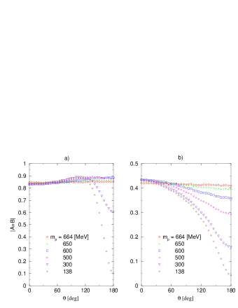
Figure 2: Angle dependence of the model hybrid decay amplitude $\cal A$ for various choices of the light meson mass, given in MeV as indicated. The smaller is the meson mass, the more important become relativistic effects and the larger is the violation of rotational symmetry. The left plot a) is for scalar constituents, and the right plot b) for fermion quarks. All points correspond to the same standard set of parameters from the first column of Table 1, labeled 2a,b, and $m_{p}$ is varied from 664 MeV down to 138 MeV. See the text for details.

Fig. 2 shows that in the case of one of the decay products being light, such as the $\pi$-meson, the decay amplitude develops practically 100 % deviation from rotational symmetry. This is clearly not acceptable and invalidates the initial picture based on a conventional choice of the model parameters, given in the first column of Table 1, labeled 2a,b. The reason is that when the light meson moves against the $z$-axis direction, its longitudinal momentum,

$$p^{+}\;=\;\sqrt{m_{p}^{2}+|\vec{p}\,|^{2}\,}\;+\;p^{3}\;,$$ (35)

becomes small. As a result of the $+$-momentum conservation, the quarks that make up this light meson must carry small fractions of the parent, hybrid momentum $h^{+}$. This configuration is suppressed if one employs parameters that would be naively considered as valid in a nonrelativistic model. In that case, the gluon decay vertex is taken directly from quantum field theory without the renormalization group form factor $f_{\lambda}$.

However, varying parameters of the model one can observe that the drastic violation of rotational symmetry is not always present. Since the number of mass parameters is 10, and varying all of them produces a huge number of combinations to investigate, one is faced with a problem of how to do a systematic test. The condition of obtaining an amplitude that does not depend on the angle $\theta$ (an infinite number of conditions) is so strong that it may easily be impossible to achieve a constant amplitude with a small set of parameters. It turns out, however, that one can obtain small variation with angle for selected sets of the parameters that are discussed below.

The results are based on a systematic computer-added manual review of about 6000 cases and subsequent numerical minimization of the amplitude variation with respect to $\theta$. Since the six dimensional integrals were carried out using Monte Carlo integration (using the procedure vegas vegas ), the accuracy of the result of integration (standard deviation output from vegas) varied from a typical 0.1 - 0.3 % to 2 % in the worst cases, and the minimization of angle dependence (Powell’s procedure Powell ) had to be carried out with a somewhat worse accuracy. Therefore, variations of the parameters that caused smaller variations of the amplitude $\cal A$ with $\theta$ than 1% could not be kept under precise control. Thus, in the obtained sets of parameters, displayed in Table 1 with three significant digits, the first is stable, while the second is highly probable and the third can be considered a result of statistical fluctuation. Figs. 3 and 4 describe the two dominant effects that we found scanning the space of parameters, and Fig. 5 shows results of the final searches for the local minima in the angle dependence. The error bars indicate the size of three standard deviations obtained in the Monte Carlo routine.

Since the decay of a hybrid into one meson as heavy as $b_{1}$ and another as light as $\pi$ is of key interest, the mass parameters $m_{h}=1.9$ GeV, $m_{b}=1.235$ GeV and $m_{p}=0.1375$ GeV are kept constant. The other seven parameters were first chosen to be (all in units of GeV, which will be omitted in the discussion) $m_{q}=0.3$, $m_{g}=0.8$, $\beta_{p}=\beta_{b}=\beta_{hg}=\beta_{hq}=0.4$ and $\lambda=4.0$. Then a code calculated $3^{7}$ cases (each for 35 different values of $\theta$) with each of the 7 parameters changing through 3 values obtained by multiplying the initial values by 0.5, 1.0, and 2.0. The resulting cases were reviewed manually and additional calculations were performed to verify trends visible in the samples. This way the two generic features illustrated on examples in Figs. 3 and 4 were identified.

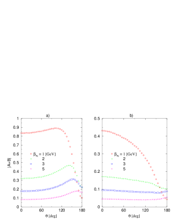
Figure 3: Angle dependence of the decay amplitude $\cal A$ with $m_{p}=0.1375$ MeV (corresponding to the lowest curves in Fig. 2) for various choices of the quark-anti-quark subsystem size in the hybrid state. The size is indicated in terms of the momentum space wave function width $\beta_{hq}$ in units of GeV, as indicated (other parameters are constant and equal to the displayed in the second column of Table 1, labeled 3a,b). The spatially smaller is the pair sub-system the larger is the relative magnitude of the relativistic decay amplitude at large angles, where Fig. 2 displayed a deficiency. See the text for details. The left graph a) is for scalar constituents and the right graph b) for fermion quarks.

Fig. 3 shows two cases, a) for scalar, and b) for fermion quarks, of what happens with the decay amplitude when one makes the quark-anti-quark pair in the hybrid smaller and smaller in size in position space ($\beta_{hq}$ grows from 1 to 5 GeV). The amplitudes are lowered at small angles while they remain more or less stable around $\theta=180^{\circ}$. This effect results from the fact that the larger domain of momenta of quarks in the hybrid is sampled by the same momentum-space wave functions of mesons, and they see less of the total probability of finding the quark-anti-quark pair in the hybrid, while the large relative momentum-tail is sampled in a similar way. Thus, the deficiency observed in Fig. 2 at large angles can disappear if the quark-anti-quark pair in the hybrid is made small in its spatial size. This is understandable since quarks are allowed to move with momenta so large that they can easily have small longitudinal fractions $x$ required in the light meson, $p$, when it flies out against $z$-axis. However, in both cases a) and b) the amplitude overshoots for large $\theta$ and a flat case is not achieved. This is easier to see in Fig. 4, which concerns the case of the lowest curves of $\beta_{hq}=5.0$ GeV from Fig. 3. Note that the remaining variation with angle is about thrice smaller in the case of fermions than in the scalar model, where it is still at the 100 % level.

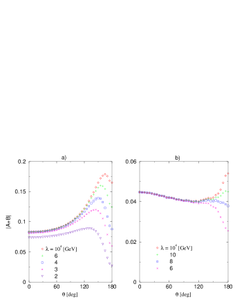
Figure 4: The result of lowering the renormalization group form factor width parameter, $\lambda$, given in GeV as indicated, in the cases with $m_{p}=0.1375$ MeV and $\beta_{hq}=5$ GeV (lowest curves in Fig. 3). The smaller is $\lambda$ the more reduced is the amplitude at large angles. The effect confirms that lowering $\lambda$ may remove the large-angle increase in the amplitude due to large $\beta_{hq}$ independently of the constituent quark spin. These results suggest that the small size of the quark-anti-quark pair in the hybrid (large $\beta_{hq}$) may be correlated with the form factor width $\lambda$ in a relativistic LF-theory through rotational symmetry. The left graph a) is for scalar constituents and the right graph b) for fermion quarks.

Fig. 4 shows another tendency in the parameter space that is related to a reduction of the overshooting due to large $\beta_{hq}$ visible in Fig. 3. Namely, the pair of quarks that originate from the hybrid decay via gluon dissociation, have their relative momentum limited by the renormalization group form factor $f_{\lambda}$. In a bare quantum field theory, $\lambda=\infty$ and no such suppression is present. However, when one lowers $\lambda$, the gluon cannot be turned into a pair of very fast moving quarks through the effective interaction, and the amplitude is suppressed again. The interplay of $\beta_{hq}$ and $\lambda$ turns out to be the key ingredient of the model that at the end allows it to produce small deviations from a constant in the amplitude $\cal A$ as a function of $\theta$.

Detailed minimization of the $\theta$-dependence leads to the four cases shown in Fig. 5. The deviation from constant was measured using the sum of squares of deviations from the average value, or maximum of the modulus of deviations from the average. The values of masses, wave function widths, and form factor parameters that produce the minimal angle variations, are given in Table 1 in the last four columns. The remarkable feature is that the required $q\bar{q}$-wave function in the hybrid has roughly the same width as the form factor in the effective vertex and this width is systematically much larger than other width parameters (see Table 1).

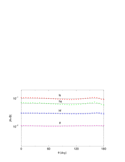
Figure 5: Four cases of decay amplitudes $\cal A$ obtained by fitting wave-function parameters and $\lambda$ so that an amplitude has the least possible variation as a function of the angle (see columns 5hs, 5ls, 5hf, 5lf in Table 1). The two upper curves are obtained in the scalar model, and the two lower curves are obtained in the fermion model. In both models, the curves differ by the optimal choice of the quark mass, which is on the order of 160-170 MeV in the cases labeled as light, and 365-375 MeV in the cases labeled as heavy. In all cases, $\beta_{hq}\sim\lambda\sim 4-5$ GeV, which suggests that the size of quark-anti-quark pair is related to the form-factor width as if the pair in the hybrid state were produced through splitting of one of two gluons in a gluonium state of the same effective theory. See details in the text.

Table 1: Parameters in Figs. 2-5 (in GeV). # a is associated with scalar particles, and b with fermions. ^† hs=heavy scalars, ls=light scalars, hf=heavy fermions, lf=light fermions. ^∗ The parameter is the same as in the left neighboring column. ^∗∗ The parameter is varying from curve to curve in the figure.

Fig. #	2a,b	3a,b	4a,b	5hs†	5ls	5hf	5lf
$m_{h}$	1.9	$s^{*}$	$s$	$s$	$s$	$s$	$s$
$m_{b}$	1.235	$s$	$s$	$s$	$s$	$s$	$s$
$m_{p}$	$v^{**}$	0.1375	$s$	$s$	$s$	$s$	$s$
$m_{q}$	0.3	$s$	$s$	.365	.175	.375	.161
$m_{g}$	0.8	$s$	$s$	1.63	2.46	.867	.845
$\beta_{p}$	0.4	$s$	$s$	.375	.363	.180	.142
$\beta_{b}$	0.4	$s$	$s$	1.01	.719	.812	.501
$\beta_{hg}$	1.0	$s$	$s$	.310	.600	.783	.854
$\beta_{hq}$	1.0	$v$	5.0	4.37	4.61	4.50	4.93
$\lambda$	10000	$s$	$v$	4.44	4.49	4.50	4.50

These results can be interpreted as that the requirement of rotational symmetry in our relativistic LF-constituent picture, forces the hybrid’s constituents to form a system made of a small-size quark-anti-quark-pair and a gluon, and the pair is about 5 to 10 times smaller than the distance between the gluon and the pair. In principle, this picture resembles a gluonium made of two gluons AP , but with one of the gluons replaced by a $q\bar{q}$-pair. The observed correlation between $\beta_{hq}$ and $\lambda$, suggests that the $q\bar{q}$-pair can be seen to originate dynamically from a decay of one gluon in a gluonium, a picture perhaps derivable from a well-defined $H_{QCD\,\lambda}$.

The amplitudes still depend on the other parameters than $\beta_{hq}$ and $\lambda$, and those can be varied in a considerable ranges causing residual changes in the angle dependence. The most pronounced effect is that flattest amplitudes are systematically arrived at when quark masses take only one of two values, about 160-170 MeV or about 370 MeV. Since in quantum field theory such as QCD one can associate the large renormalization group scale $\lambda$ with the smaller rather than the larger quark masses, it appears to be a remarkably consistent feature of the effective constituent approach that the lighter quark mass cases lead to amplitudes that vary less in $\theta$ than for the heavier quarks.

V Conclusion

The numerical study described in this work shows that constraints imposed by requirements of rotational symmetry on parameters of a crude LF constituent model of a relativistic decay of a hybrid can be satisfied even if the model assumes that only lowest effective-particle Fock-space components are included in the wave functions of the participating hadrons. Since the boost symmetry is kinematical in the LF quantum field theory, and the model is built to be compatible with the rules of renormalized LF Hamiltonian dynamics for effective particles, it is interesting that a self-consistent picture of the hybrid state in such a simple class of models emerges without major obstacles as soon as one introduces the right width $\lambda$ of the effective vertex form factor. The key renormalization group aspect of the constituent model is that the special-relativity symmetry constraints are satisfied only approximately. The accuracy is expected to improve when the renormalization group equations for effective constituent theory are solved including higher order terms than the first considered here, and when the resulting constituent dynamics is solved precisely, which together would be analogous to restoring rotational symmetry in lattice gauge theory.

The physical picture of a hybrid meson that one can now attempt to uncover by performing the detailed calculations in QCD, has the following spatial structure. A quark-anti-quark-pair of small size and a gluon move around a common center, and this system of two objects is not far from a gluonium. In the latter case, one has a second gluon, instead of the small quark-anti-quark pair. Solution of the QCD Hamiltonian eigenvalue problem has a chance to be approximated this way only in terms of renormalized effective particles, for which the similarity renormalization group width parameter is comparable to the size of the wave-function parameters. The key difficulty of the calculation will be to properly include the constituent-gluon spin.

*

Appendix A

In the model without gluon spin, one substitutes

$$S_{QCD}(i,j)=S_{p}(i,j)=S_{b}(i,j)=S_{h}(i,j)=S(i,j)\;,$$ (36)

and obtains

$${\cal A}(p,b,h)=(-1){2\over 3}{1\over\sqrt{2}}{g_{\lambda}\over(16\pi^{3})^{2}}\int{dx_{14}d^{2}\kappa^{\perp}_{14}\over x_{14}(1-x_{14})}\int{dx_{52}d^{2}\kappa^{\perp}_{52}\over x_{52}(1-x_{52})}{1\over x_{3}}$$

$$\times N_{p}N_{b}N_{h}\psi^{*}_{p}(1,4)\psi^{*}_{b}(5,2)T(1,2,4,5)\left[A(1,2,4,5)+B(1,2,4,5)\right]$$

$$=-{16\over 3}{g_{\lambda}\over(16\pi^{3})^{2}}\int{d^{3}k_{b}\over{\cal M}_{b}}\int{d^{3}k_{p}\over{\cal M}_{p}}{1\over x_{3}}N_{p}N_{b}N_{h}\psi^{*}_{p}(\vec{k}_{14})\psi^{*}_{b}(\vec{k}_{52})T(1,2,4,5)\left[A(1,2,4,5)+B(1,2,4,5)\right]\;,$$ (37)

where

$$A(1,2,4,5)=\psi_{h}(1,2,3)f_{\lambda}({\cal M}^{2}_{45})\;,$$ (38)

$$B(1,2,4,5)=\psi_{h}(5,4,3)f_{\lambda}({\cal M}^{2}_{12})\;,$$ (39)

and

$$T(1,2,4,5)=Tr\left[S^{\dagger}(1,4)S(1,2)S^{\dagger}(5,2)S(5,4)\right]\;,$$ (40)

with $S(i,j)=\bar{u}_{i}v_{j}$, or

$$S(i,j)={\left[m_{q}(x_{i}-x_{j})\sigma^{3}+(x_{j}k_{i}^{\perp}-x_{i}k_{j}^{\perp})\sigma^{\perp}\right]i\sigma^{2}\over\sqrt{x_{i}x_{j}}}\;,$$ (41)

which give $T(1,2,4,5)$ equal to

$$2\,{(\vec{y}_{1}\vec{y}_{2})(\vec{y}_{3}\vec{y}_{4})-(\vec{y}_{1}\vec{y}_{3})(\vec{y}_{2}\vec{y}_{4})+(\vec{y}_{1}\vec{y}_{4})(\vec{y}_{2}\vec{y}_{3})\over x_{1}x_{2}x_{3}x_{4}}\;,$$ (42)

where

$$\vec{y}_{1} = \left[m_{q}(x_{1}-x_{4}),x_{4}k_{1}^{\perp}-x_{1}k_{4}^{\perp}\right]\;,$$

$$\vec{y}_{2} = \left[m_{q}(x_{1}-x_{2}),x_{2}k_{1}^{\perp}-x_{1}k_{2}^{\perp}\right]\;,$$

$$\vec{y}_{3} = \left[m_{q}(x_{5}-x_{2}),x_{2}k_{5}^{\perp}-x_{5}k_{2}^{\perp}\right]\;,$$

$$\vec{y}_{4} = \left[m_{q}(x_{5}-x_{4}),x_{4}k_{5}^{\perp}-x_{5}k_{4}^{\perp}\right]\;.$$ (43)

An alternative expression is

$$T(1,2,4,5) = ({\cal M}^{2}_{14}-4m_{q}^{2})({\cal M}^{2}_{52}-4m_{q}^{2})$$ (44)

$$- ({\cal M}^{2}_{15}-4m_{q}^{2})({\cal M}^{2}_{42}-4m_{q}^{2})$$

$$+ ({\cal M}^{2}_{12}-4m_{q}^{2})({\cal M}^{2}_{45}-4m_{q}^{2})\;.$$

In both parts of the amplitude, $A$ and $B$, one has $x_{p}=p^{+}/h^{+}$, $x_{b}=b^{+}/h^{+}=1-x_{p}$. In meson $p$, one has $\vec{k}_{14}\equiv\vec{k}_{p}$, so that ${\cal M}_{14}={\cal M}_{p}=2\sqrt{m_{q}^{2}+\vec{k}_{p}^{\,2}}$, and the following relations hold: $x_{14}=(\sqrt{m_{q}^{2}+\vec{k}^{\,2}_{p}}+k_{p}^{3})/{\cal M}_{p}$, $k_{1}^{+}=x_{14}p^{+}$, $x_{1}=x_{14}x_{p}$, $k_{4}^{+}=(1-x_{14})p^{+}$, $x_{4}=(1-x_{14})x_{p}$, $k_{1}^{\perp}=x_{14}p^{\perp}+k_{p}^{\perp}$, $k_{4}^{\perp}=(1-x_{14})p^{\perp}-k_{p}^{\perp}$. In meson $b$, one has $\vec{k}_{52}\equiv\vec{k}_{b}$, so that ${\cal M}_{b}=2\sqrt{m_{q}^{2}+\vec{k}_{b}^{\,2}}={\cal M}_{52}$, and the analogous relations are: $x_{52}=(\sqrt{m_{q}^{2}+\vec{k}^{\,2}_{b}}+k_{b}^{3})/{\cal M}_{b}$, $k_{5}^{+}=x_{52}b^{+}$, $x_{5}=x_{52}x_{b}$, $k_{2}^{+}=(1-x_{52})b^{+}$, $x_{2}=(1-x_{52})x_{b}$, $k_{5}^{\perp}=x_{52}b^{\perp}+k_{b}^{\perp}$, $k_{2}^{\perp}=(1-x_{52})b^{\perp}-k_{b}^{\perp}$. Evaluating the quarks’ invariant masses in the hybrid and decay vertex, one then obtains

$${\cal M}^{2}_{12} = (x_{1}+x_{2})\left[{k_{1}^{\perp\,2}+m^{2}_{q}\over x_{1}}+{k_{2}^{\perp\,2}+m^{2}_{q}\over x_{2}}\right]$$ (45)

$$- (k_{1}^{\perp}+k_{2}^{\perp})^{2},$$

and

$${\cal M}^{2}_{54} = (x_{5}+x_{4})\left[{k_{5}^{\perp\,2}+m^{2}_{q}\over x_{5}}+{k_{4}^{\perp\,2}+m^{2}_{q}\over x_{4}}\right]$$ (46)

$$- (k_{5}^{\perp}+k_{4}^{\perp})^{2}.$$

In the part $A$ of the decay amplitude, one has

$$\vec{k}^{\,2}_{q}={\cal M}^{2}_{12}/4-m_{q}^{2}\;,$$ (47)

and

$$\vec{k}^{\,2}_{g}={\left[{\cal M}^{2}_{123}-\left({\cal M}_{12}+m_{g}\right)^{2}\right]\left[{\cal M}^{2}_{123}-\left({\cal M}_{12}-m_{g}\right)^{2}\right]\over 4{\cal M}^{2}_{123}}\;,$$ (48)

where

$${\cal M}^{2}_{123} = {k_{1}^{\perp\,2}+m^{2}_{q}\over x_{1}}+{k_{2}^{\perp\,2}+m^{2}_{q}\over x_{2}}$$

$$+ {(k_{1}+k_{2})^{\perp\,2}+m^{2}_{g}\over 1-x_{1}-x_{2}}-(k_{1}+k_{2}+k_{3})^{\perp\,2}\;.$$

Similarly, in the part $B$, one has

$$\vec{k}^{\,2}_{q}={\cal M}^{2}_{54}/4-m_{q}^{2}\;,$$ (50)

and

$$\vec{k}^{\,2}_{g}={\left[{\cal M}^{2}_{543}-\left({\cal M}_{54}+m_{g}\right)^{2}\right]\left[{\cal M}^{2}_{543}-\left({\cal M}_{54}-m_{g}\right)^{2}\right]\over 4{\cal M}^{2}_{543}}\;,$$ (51)

where

$${\cal M}^{2}_{543} = {k_{5}^{\perp\,2}+m^{2}_{q}\over x_{5}}+{k_{4}^{\perp\,2}+m^{2}_{q}\over x_{4}}$$

$$+ {(k_{5}+k_{4})^{\perp\,2}+m^{2}_{g}\over 1-x_{5}-x_{4}}-(k_{5}+k_{4}+k_{3})^{\perp\,2}\;.$$

References

- (1) N. Isgur, R. Kokoski, J. Paton, Phys. Rev. Lett. 54 869 (1985); F. Iddir, A. Le Yaouanc, L. Oliver, O. Pene, J.C. Raynal, Phys. Lett. B207, 325 (1988); P. R. Page, Phys. Lett. B402, 183 (1997).
- (2) K. J. Juge, J. Kuti, C. J. Morningstar, Nucl. Phys. Proc. Suppl. 63, 326 (1998); K. J. Juge, J. Kuti, C. J. Morningstar, Phys. Rev. Lett. 82, 4400 (1999).
- (3) A. P. Szczepaniak, E. S. Swanson, Phys. Rev. D55, 3987 (1997); E. S. Swanson, A. P. Szczepaniak, Phys. Rev. D59, 014035 (1999); A. P. Szczepaniak, E. S. Swanson, Phys. Rev. D65, 025012 (2002).
- (4) T. Barnes, F. E. Close, F. de Viron, J. Weyers, Nucl. Phys. B224, 241 (1983); M. S. Chanowitz, S. R. Sharpe, Nucl. Phys. B222, 211 (1983); P. Hasenfratz, R. R. Horgan, J. Kuti, J. M. Richard, Phys. Lett. B95, 299 (1980); D. Horn, J. Mandula, Phys. Rev. D17, 898 (1978); N. Isgur, J. Paton, Phys. Rev. D31, 2910 (1985); A. W. Thomas, A. P. Szczepaniak, Phys. Lett. B526, 72 (2002).
- (5) A. Le Yaouanc, L. Oliver, O. Pene, J. C. Raynal, S. Ono, Z. Phys. C28, 309 (1985); R. Kokoski, N. Isgur, Phys. Rev. D35, 907 (1987); F. E. Close, P. R. Page, Nucl. Phys. B443, 233 (1995); E. S. Swanson, A. P. Szczepaniak, Phys. Rev. D56, 5692 (1997); P. R. Page, E. S. Swanson, A. P. Szczepaniak, Phys. Rev. D59, 034016 (1999).
- (6) G. P. Lepage, S. J. Brodsky, Phys. Rev. D22, 2157 (1980).
- (7) K. G. Wilson et al., Phys. Rev. D49, 6720 (1994); and references therein.
- (8) St. D. Głazek, Phys. Rev. D63, 116006 (2001); and references therein.
- (9) St. D. Głazek, T. Masłowski, Phys. Rev. D65, 065011 (2002).
- (10) See e.g. St. D. Głazek, M. Wiȩckowski, hep-th/0204171.
- (11) A. P. Szczepaniak, C. R. Ji, S. R. Cotanch, Phys. Rev. D52, 5284 (1995); ibid. Phys. Rev. C52, 2738 (1995).
- (12) J. R. Finger, J. E. Mandula, Nucl. Phys. B199, 168 (1982); S. L. Adler, A. C. Davis, Nucl. Phys. B244, 469 (1984); A. Le Yaouanc, et al., Phys. Rev. D31, 137 (1985); R. Alkofer, P. A. Amundsen, Nucl. Phys. B306, 305 (1988). A. P. Szczepaniak, E. S. Swanson, Phys. Rev. D55, 1578 (1997)
- (13) See e.g. J. Kogut, L. Susskind, Phys. Rep. C8, 75 (1973).
- (14) S. Godfrey, N. Isgur, Phys. Rev. D32, 189 (1985); S. Capstick, N. Isgur, Phys. Rev. D34, 2809 (1986).
- (15) B. L. G. Bakker, L. A. Kondratyuk, M. V. Terent’ev, Nucl. Phys. B158 (1979) 497; L. A. Kondratyuk, M. V. Terentev, Sov. J. Nucl. Phys. 31, 561 (1980). F. Coester, W. N. Polyzou, Phys. Rev. D26, 1348 (1982).
- (16) See e.g. P. Danielewicz, J. M. Namysłowski, Phys. Lett. B81, 110 (1979).
- (17) G. P. Lepage, Vegas: An adaptive multidimensional integration program, CLNS-80/447, March 1980.
- (18) W. H. Press, B. P. Flannery, S. A. Teukolsky, and W. T. Vettering, Numerical Recipes, The Art of Scientific Computing (Cambridge University Press, New York, 1986).
- (19) B. H. Allen, R. J. Perry, Phys. Rev. D62, 025005 (2000).