Charmless Three-body Baryonic $B$ Decays

Abstract

Motivated by recent data on $B\to p\bar{p}K$ decay, we study various charmless three-body baryonic $B$ decay modes, including $\Lambda\bar{p}\pi$, $\Sigma^{0}\bar{p}\pi$, $p\bar{p}\pi$, $p\bar{p}\overline{K}{}^{0}$, in a factorization approach. These modes have rates of order $10^{-6}$. There are two mechanisms for the production of baryon pairs: current-produced and transition. The behavior of decay spectra from these baryon production mechanisms can be understood by using QCD counting rules. Predictions on rates and decay spectra can be checked in the near future.

I Introduction

The Belle collaboration recently reported the observation of $B^{-}\to p\bar{p}K^{-}$ decay, the first ever charmless baryonic $B$ decay mode, giving ${\mathcal{B}}=(4.3^{+1.1}_{-0.9}\pm 0.5)\times 10^{-6}$ Abe:2002ds . Three-body baryonic decay in $b\to c$ transitions have been observed Anderson:2000tz previously, following a suggestion by Dunietz Dunietz:1998uz . It is interesting to compare the charmless case to the charmful one and also to charmless two-body modes such as $B^{0}\to p\bar{p}$, which has ${\mathcal{B}}<1.2\times 10^{-6}$ Abe:2002er .

It has been pointed out that reduced energy release (e.g. by a fast recoiling meson) would favor the generation of baryon pair and thus three-body baryonic modes could be enhanced over two-body rates Hou:2000bz . One of the signatures would be (baryon pair) threshold enhancement in the three-body baryonic modes. In our previous study of $B^{0}\to D^{*-}p\bar{n}$ Chua:2001vh , we assumed factorization and obtained up to 60% of experimental rate from the vector current contribution. The decay spectrum exhibits threshold enhancement. The same threshold enhancement effect was predicted for the charmless $\rho p\bar{n}$ mode, giving ${\mathcal{B}}\sim 10^{-6}$ Chua:2001xn . It is interesting that the newly observed $p\bar{p}K$ mode shows such a threshold enhancement Abe:2002ds . With this encouragement we extend our study to charmless modes such as $\Lambda\bar{p}\pi$, $\Sigma\bar{p}\pi$, $p\bar{p}\pi^{-}$, $p\bar{p}K^{-}$ and $p\bar{p}\overline{K}{}^{0}$. These modes are interesting not just by their (possibly) large rates, but also by their accessibility. Some of these modes are studied in a recent work Cheng:2001tr that utilizes a factorization and pole model approach.

In Sec. II, we extend the factorization approach to the charmless case, where one now has two mechanisms for baryon pair production. In Sec. III, we discuss baryonic form factors and their associated Quantum Chromo-Dynamics (QCD) counting rules Brodsky:1974vy . In Sec. IV, the formulation is applied to the above mentioned charmless modes. The threshold enhancement phenomenon is found to be closely related to the QCD counting rules. Discussion and conclusion are given in Sec. V, while some useful formulas are collected in an appendix.

Figure 1: (a) The current-produced (${\mathcal{J}}$) and (b) transition (${\mathcal{T}}$) diagrams for $B^{-}\to p\bar{p}K^{-}$ decay.

II Factorization

In this section we extend the factorization approach used in Refs. Chua:2001vh ; Chua:2001xn to charmless decay modes. Under the factorization assumption, the three-body baryonic $B$ decay matrix element is separated into either a current-produced baryon pair ($\mathcal{J}$) part together with a $B$ to recoil meson transition part, or a $B$ to baryon pair transition ($\mathcal{T}$) part together with a current-produced recoil meson part. As an example, the current-produced and transition diagrams for $B^{-}\to p\bar{p}K^{-}$ decay are depicted in Fig. 1.

Table 1: The coefficients $a_{i}$ for $b\to s~{}[b\to d\,]$ from Cheng:1999xj . Values for $a_{3}-a_{9}$ are in units of $10^{-4}$.

	$N_{c}=2$	$N_{c}=3$	$N_{c}=\infty$
$a_{1}$	0.99 [0.99]	1.05 [1.05]	1.17 [1.17]
$a_{2}$	0.22 [0.22]	0.02 [0.02]	$-0.37~{}[-0.37]$
$a_{3}$	$-4.5-23\,i~{}[-2-20\,i]$	$72.7-0.3\,i~{}[73+0.3\,i]$	$227+45\,i~{}[223+41\,i]$
$a_{4}$	$-349.5-113.5\,i~{}[-338.5-101.5\,i]$	$-387.3-121\,i~{}[-375.7-108.3\,i]$	$-463-136\,i~{}[-450-122\,i]$
$a_{5}$	$-166-23\,i~{}[-164-20\,i]$	$-66-0.3\,i~{}[-66+0.3\,i]$	$134+45\,i~{}[130+41\,i]$
$a_{6}$	$-533-113.5\,i~{}[-523-101.5\,i]$	$-555.3-121\,i~{}[-544.7-108.3\,i]$	$-600-136\,i~{}[-588-122\,i]$
$a_{9}$	$-86.8-2.7\,i~{}[-86.6-2.5\,i]$	$-92.6-2.7\,i~{}[-92.4-2.5\,i]$	$-104.3-2.7\,i~{}[-104.1-2.5\,i]$

In charmless decay modes, we need to use the effective Hamiltonian consisting of operators and Wilson coefficients, which is standard and can be found, for example, in Refs. Cheng:1999xj ; Ali:1998eb . In this work, we concentrate on the dominant terms. The factorization formula for the decay process $B\to X\,Y$, where $(X,Y)=(h,{\rm\bf B}\overline{\rm\bf B}^{\prime})$ with $h$ being a light meson and ${\rm\bf B}\overline{\rm\bf B}^{\prime}$ a baryon pair or vice versa is given by

$${\cal M}\left(B\to X\,Y\right) = \frac{G_{F}}{\sqrt{2}}\bigg{\{}V_{ub}V_{uq}^{*}[a_{1}(\bar{q}u)_{V-A}\otimes(\bar{u}b)_{V-A}+a_{2}(\bar{u}u)_{V-A}\otimes(\bar{q}b)_{V-A}]$$ (1)

$$-V_{tb}V_{tq}^{*}\Big{[}a_{3}\sum_{q^{\prime}}(\bar{q}^{\prime}q^{\prime})_{V-A}\otimes(\bar{q}b)_{V-A}+a_{4}\sum_{q^{\prime}}(\bar{q}q^{\prime})_{V-A}\otimes(\bar{q}^{\prime}b)_{V-A}$$

$$\qquad+a_{5}\sum_{q^{\prime}}(\bar{q}^{\prime}q^{\prime})_{V+A}\otimes(\bar{q}b)_{V-A}-2a_{6}\sum_{q^{\prime}}(\bar{q}q^{\prime})_{S+P}\otimes(\bar{q}^{\prime}b)_{S-P}$$

$$\qquad+\frac{3}{2}a_{9}\sum_{q^{\prime}}e_{q^{\prime}}(\bar{q}^{\prime}q^{\prime})_{V-A}\otimes(\bar{q}b)_{V-A}+\dots\Big{]}\bigg{\}}\,,$$

where ${\cal O}_{1}\otimes{\cal O}_{2}$ stands for $\langle X|{\cal O}_{1}|0\rangle\langle Y|{\cal O}_{2}|B\rangle$. The coefficients $a_{i}$ are defined in terms of the effective Wilson coefficients $c^{\rm eff}_{i}$ as $a_{i={\rm odd}}\equiv c^{\rm eff}_{i}+c^{\rm eff}_{i+1}/N_{c}$ and $a_{i={\rm even}}\equiv c^{\rm eff}_{i}+c^{\rm eff}_{i-1}/N_{c}$. We stress that $c^{\rm eff}_{i}$ are renormalization scale and scheme independent, as vertex and penguin corrections are included Cheng:1999xj . Their values are given in Table 1. In this work we use the $N_{c}=3$ case, while the $N_{c}=2,\infty$ cases are shown to indicate non-factorizable effects.

III Form Factors and QCD Counting Rules

In this section, we first discuss the meson form factors used in this work. We then turn to discuss baryonic form factors, especially the implication of QCD counting rules.

III.1 Meson Form Factors

The decay constant $f_{h}$ of the pseudoscalar meson $h$ is defined as

$$\langle h(p_{h})|\bar{q}\gamma^{\mu}(1-\gamma_{5})\,q^{\prime}|0\rangle=i\,f_{h}\,p^{\mu}_{h}\,.$$ (2)

These parameters and quark masses are taken from Ref. Ali:1998eb .

We also need $0^{-}\to 0^{-}$ form factors defined as follows:

$$\langle h\,(p_{h})\left|\bar{q}\gamma^{\mu}(1-\gamma_{5})\,b\right|B(p_{B})\rangle = \biggl{[}(p_{B}+p_{h})^{\mu}-\frac{m_{B}^{2}-m_{h}^{2}}{(p_{B}-p_{h})^{2}}\,(p_{B}-p_{h})^{\mu}\biggr{]}\,F^{B\to h}_{1}(t)$$ (3)

$$\qquad\qquad\qquad+\frac{m_{B}^{2}-m_{h}^{2}}{(p_{B}-p_{h})^{2}}\,(p_{B}-p_{h})^{\mu}\,F^{B\to h}_{0}(t)\,.$$

We use the so-called MS form factors, which take the following form Melikhov:2000yu :

$$F^{B\to h}_{1}(t) = \frac{F^{B\to h}_{1}(0)}{(1-t/M_{V}^{2})[1-\sigma_{1}\,t/M_{V}^{2}+\sigma_{2}\,t^{2}/M_{V}^{4}]}\,,$$ (4)

$$F^{B\to h}_{0}(t) = \frac{F^{B\to h}_{0}(0)}{1-\sigma_{1}\,t/M_{V}^{2}+\sigma_{2}\,t^{2}/M_{V}^{4}}\,,$$ (5)

where $M_{V}=5.42\ (5.32)$ GeV for $h=K(\pi)$. Other parameters are given in Table 2.

Table 2: Relevant parameters for the $B\to K,\pi$ transition form factors of Eqs. (4) and (5).

	$F^{B\to K}_{1}$	$F^{B\to K}_{0}$	$F^{B\to\pi}_{1}$	$F^{B\to\pi}_{0}$
$F_{1,0}^{B\to h}(0)$	0.36	0.36	0.29	0.29
$\sigma_{1}$	0.43	0.70	0.48	0.76
$\sigma_{2}$	—	0.27	—	0.28

III.2 Baryon Form Factors

Factorization introduces two types of matrix elements containing the baryon pair: $\langle{\rm\bf B}\overline{\rm\bf B}^{\prime}|V(A)|0\rangle$ involving vector ($V$) or axial vector ($A$) current-produced baryon pair, and $\langle{\rm\bf B}\overline{\rm\bf B}^{\prime}|V(A)|B\rangle$ involving the $B\to{\rm\bf B}\overline{\rm\bf B}^{\prime}$ transition.

For the current-produced matrix elements, we have

$$\langle{\rm\bf B}\overline{\rm\bf B}^{\prime}|V_{\mu}|0\rangle = \bar{u}(p_{\rm\bf B})\left\{F_{1}(t)\gamma_{\mu}+i\frac{\,F_{2}(t)}{m_{\rm\bf B}+m_{\overline{\rm\bf B}^{\prime}}}\sigma_{\mu\nu}\left(p_{\rm\bf B}+p_{\overline{\rm\bf B}^{\prime}}\right)^{\nu}\right\}v(p_{\overline{\rm\bf B}^{\prime}})$$ (6)

$$= \bar{u}(p_{\rm\bf B})\left\{(F_{1}+F_{2})\gamma_{\mu}+\frac{\,F_{2}(t)}{m_{\rm\bf B}+m_{\overline{\rm\bf B}^{\prime}}}\left(p_{\overline{\rm\bf B}^{\prime}}-p_{\rm\bf B}\right)^{\mu}\right\}v(p_{\overline{\rm\bf B}^{\prime}})\,,$$

$$\langle{\rm\bf B}\overline{\rm\bf B}^{\prime}|A_{\mu}|0\rangle = \bar{u}(p_{\rm\bf B})\left\{g_{A}\left(t\right)\gamma_{\mu}+\frac{h_{A}\left(t\right)}{m_{\rm\bf B}+m_{\overline{\rm\bf B}^{\prime}}}\,\left(p_{\rm\bf B}+p_{\overline{\rm\bf B}^{\prime}}\right)_{\mu}\right\}\gamma_{5}\,v(p_{\overline{\rm\bf B}^{\prime}})\,,$$ (7)

where $F_{1,2}$ are the induced vector form factors, $g_{A}$ the axial form factor, and $h_{A}$ the induced pseudoscalar form factor. We have used Gordon decomposition to obtain the second line of Eq. (6). Note that $t\equiv(p_{\rm\bf B}+p_{\overline{\rm\bf B}^{\prime}})^{2}\equiv m^{2}_{{\mathbf{B}}\overline{\mathbf{B}}^{\prime}}$ is nothing but the ${\mathbf{B}}\overline{\mathbf{B}}^{\prime}$ pair mass.

According to QCD counting rules Brodsky:1974vy , both the vector form factor $F_{1}$ and the axial form factor $g_{A}$, supplemented with the leading logs, behave as $1/t^{2}$ in the $t\to\infty$ limit, since we need two hard gluons to distribute large momentum transfer. $F_{2}$ and $h_{A}$ behave as $1/t^{3}$, acquiring an extra $1/t$ due to helicity flip. In the electromagnetic current case, the asymptotic form has been confirmed by many experimental measurements of the nucleon magnetic (Sachs) form factor $G_{M}=F_{1}+F_{2}$, over a wide range of momentum transfers in the space-like region. The asymptotic behavior for $G^{p}_{M}$ also seems to hold in the time-like region, as reported by the Fermilab E760 experiment Armstrong93 for $8.9$ GeV${}^{2}<t<13$ GeV². Another Fermilab experiment, E835, has recently reported Ambrogiani:1999bh $G^{p}_{M}$ for momentum transfers up to $\sim 14.4$ GeV². An empirical fit of $\left|G^{p}_{M}\right|=Ct^{-2}[\ln({t}/{Q_{0}^{2}})]^{2}$, is in agreement with the QCD counting rule prediction.

Table 3: Relations of baryon form factors $F_{1}+F_{2}$ and $g_{A}$ with the nucleon magnetic form factors $G_{M}^{p,n}$.

${\mathbf{B}}\overline{\mathbf{B}}^{\prime}$	$V,\,A$	SU(3)	$F_{1}+F_{2}$	$g_{A}(t\to\infty)$
$p\bar{n}$	$(\bar{u}d)_{V,A}$	$(F+D)_{V,A}$	$G^{p}_{M}-G^{n}_{M}$	$\frac{5}{3}\,G^{p}_{M}+G^{n}_{M}$
$\Lambda\bar{p}$	$(\bar{s}u)_{V,A}$	$\left(-\sqrt{\frac{3}{2}}\,F-\sqrt{\frac{1}{6}}\,D\right)_{V,A}$	$-\sqrt{\frac{3}{2}}\,G^{p}_{M}$	$-\sqrt{\frac{3}{2}}\,G^{p}_{M}$
$\Sigma^{0}\bar{p}$	$(\bar{s}u)_{V,A}$	$\frac{1}{\sqrt{2}}\,\left(D-F\right)_{V,A}$	$\frac{-1}{\sqrt{2}}\left(G_{M}^{p}+2\,G_{M}^{n}\right)$	$\frac{1}{3\,\sqrt{2}}(G_{M}^{p}+6\,G_{M}^{n})$
$p\bar{p}$	$(\bar{u}u)_{V,A}$	$(F+D+S)_{V,A}$	$G^{p}_{M}-G^{n}_{M}+S_{V}$	$\frac{4}{3}\,G^{p}_{M}-G^{n}_{M}$
$p\bar{p}$	$(\bar{d}d)_{V,A}$	$S_{V,A}$	$S_{V}$	$-\frac{1}{3}\,G^{p}_{M}-2G^{n}_{M}$
$p\bar{p}$	$(\bar{s}s)_{V,A}$	$(D-F+S)_{V,A}$	$-G^{p}_{M}-2G^{n}_{M}+S_{V}$	0
$p\bar{p}$	$(\bar{u}u+\bar{d}d+\bar{s}s)_{V,A}$	$(2\,D+3\,S)_{V,A}$	$3\,(-G^{n}_{M}+S_{V})$	$G^{p}_{M}-3\,G^{n}_{M}$
$p\bar{p}$	$(e_{u}\,\bar{u}u+e_{d}\,\bar{d}d+e_{S}\,\bar{s}s)_{V,A}$	$(F+D/3)_{V,A}$	$G^{p}_{M}$	$G^{p}_{M}$

The current induced form factors $F_{1}+F_{2}$ and $g_{A}$ can be related by means of the SU(3) decomposition form factors $F_{V,A}$, $D_{V,A}$ and $S_{V,A}$ (with $S_{V,A}$ appearing only in the non-traceless current case), as shown in Table 3. It is well known that $F_{V}$ and $D_{V}$ can be expressed by the nucleon magnetic form factors $G_{M}^{p,n}$,

$$F_{V}=G_{M}^{p}+\frac{1}{2}\,G_{M}^{n}\,,\ \ \ \ \ D_{V}=-\frac{3}{2}\,G_{M}^{n}.$$ (8)

As the first term $F_{1}+F_{2}$ in Eq. (6) can be related to nucleon magnetic Sachs form factor $G_{M}$, similarly the second term $F_{2}$ can be related to $(G_{E}-G_{M})/[t/(m_{\bf B}+m_{\bf B^{\prime}})^{2}-1]$, where $G_{E}$ is the nucleon electric Sachs form factor. Since we do not have enough data on time-like nucleon $G_{E}$, we concentrate on the $F_{1}+F_{2}$ term as we did in Ref. Chua:2001vh . We may in fact gain information on $G_{E}$ by reversing our present analysis on these three-body baryonic $B$ decays in the future when more data become available.

The nucleon magnetic form factors are fitted to available data in Ref. Chua:2001vh by

$$G_{M}^{p}(t)=\sum^{5}_{i=1}\frac{x_{i}}{t^{i+1}}\left[\ln\left(\frac{t}{\Lambda_{0}^{2}}\right)\right]^{-\gamma} G_{M}^{n}(t)=-\sum^{2}_{i=1}\frac{y_{i}}{t^{i+1}}\left[\ln\left(\frac{t}{\Lambda_{0}^{2}}\right)\right]^{-\gamma}\,,$$ , (9)

where $\gamma=2.148$, $x_{1}=420.96$ GeV⁴, $x_{2}=-10485.50$ GeV⁶, $x_{3}=106390.97$ GeV⁸, $x_{4}=-433916.61$ GeV¹⁰, $x_{5}=613780.15$ GeV¹², $y_{1}=236.69$ GeV⁴, $y_{2}=-579.51$ GeV⁶, and $\Lambda_{0}=0.3$ GeV. They satisfy QCD counting rules and describe time-like electromagnetic data such as $e^{+}e^{-}\to N\overline{N}$ suitably well. We have real and positive (negative) time-like $G^{p(n)}_{M}$ Hammer:1996kx ; Baldini:1999qn . It is interesting to note the alternating signs of the $x_{i}$ and $y_{i}$ parameters, and that only two terms are needed to describe the neutron magnetic form factor Chua:2001vh .

The time-like form factors related to $S_{V}$, $F_{A}$, $D_{A}$, $S_{A}$ are not yet measured. It is noted in Ref. Cheng:2001tr that the asymptotic behavior of baryon form factors studied in the 80s may be useful. Their asymptotic behavior as $t\to\infty$ can be described by two form factors depending on the reacting quark having parallel or anti-parallel spin with respect to baryon spin Brodsky:1980sx . By expressing these two form factors in terms of $G_{M}^{p,n}$ as $t\to\infty$, one has

$$S_{V} \to G_{M}^{p}+2\,G_{M}^{n},$$

$$F_{A} \to \frac{2}{3}\,G_{M}^{p}-\frac{1}{2}\,G_{M}^{n},$$

$$D_{A} \to G_{M}^{p}+\frac{3}{2}\,G_{M}^{n},$$

$$S_{A} \to -\frac{1}{3}\,G_{M}^{p}-2\,G_{M}^{n}.$$ (10)

Since these relations only hold for large $t$, it implies relations on the leading terms of these form factors. In general more terms may be needed. In analogy to the neutron magnetic form case, we express these form factors up to the second term

$$S_{V}(t) \equiv \left(\frac{s_{1}}{t^{2}}+\frac{s_{2}}{t^{3}}\right)\left[\ln\left(\frac{t}{\Lambda_{0}^{2}}\right)\right]^{-\gamma},$$

$$F_{A}(t) \equiv \left(\frac{\tilde{f}_{1}}{t^{2}}+\frac{\tilde{f}_{2}}{t^{3}}\right)\left[\ln\left(\frac{t}{\Lambda_{0}^{2}}\right)\right]^{-\gamma},$$

$$D_{A}(t) \equiv \left(\frac{\tilde{d}_{1}}{t^{2}}+\frac{\tilde{d}_{2}}{t^{3}}\right)\left[\ln\left(\frac{t}{\Lambda_{0}^{2}}\right)\right]^{-\gamma},$$

$$S_{A}(t) \equiv \left(\frac{\tilde{s}_{1}}{t^{2}}+\frac{\tilde{s}_{2}}{t^{3}}\right)\left[\ln\left(\frac{t}{\Lambda_{0}^{2}}\right)\right]^{-\gamma}.$$ (11)

The asymptotic relations of Eq. (10) imply $s_{1}=x_{1}-2y_{1}$, $\tilde{f}_{1}=2\,x_{1}/3+y_{1}/2$, $\tilde{d}_{1}=x_{1}-3\,y_{1}/2$ and $\tilde{s}_{1}=-x_{1}/3+2\,y_{1}$.

The coefficients of the second terms are undetermined due to the lack of data. However, we can use the axial vector ($g^{pn}_{A}=F_{A}+D_{A}$) contribution in $B^{0}\rightarrow D^{*-}p\bar{n}$ decay to constrain $\tilde{f}_{2}$ and $\tilde{d}_{2}$. The part of the branching fraction ${\cal B}(B^{0}\rightarrow D^{*-}p\bar{n})=(14.5^{+3.4}_{-3.0}\pm 2.7)\times 10^{-4}$ Anderson:2000tz arising from the vector current has been calculated to give ${\mathcal{B}}_{V}\sim 7\times 10^{-4}$ Chua:2001vh . We find for $\tilde{f}_{2}+\tilde{d}_{2}=-2110\ {\rm GeV}^{6}$, the branching fraction coming from the axial current ${\cal B}_{A}(B^{0}\rightarrow D^{*-}p\bar{n})\sim 12.7\times 10^{-4}$, and the sum ${\cal B}_{V}+{\cal B}_{A}$ is within the measurement range. Had we used the asymptotic form of Eq. (10) for $g^{pn}_{A}$ in the whole time-like region, we would obtain ${\cal B}_{A}\sim 1.0\times 10^{-4}$, which is too small.

In this work we take

$$\tilde{f}_{2}+\tilde{d}_{2}\equiv\tilde{z}=-2110~{}{\rm GeV}^{6}\,,$$ (12)

and $s_{2}=\tilde{s}_{2}=0$ for simplicity, since there is no data to constrain these yet. It is interesting to note that the asymptotic relations give vanishing results for $\langle p\bar{p}|(\bar{s}s)_{V,A}|0\rangle\ (\sim D_{V,A}-F_{V,A}+S_{V,A})$, as one can see from Table 3 and Eq. (10). This can be understood as OZI suppression. We still have a vanishing $\langle p\bar{p}|(\bar{s}s)_{A}|0\rangle$ for smaller $t$, if we take $\tilde{d}_{2}=\tilde{f}_{2}=\tilde{z}/2$. Since there is no point to advocate a large $\bar{s}s$ form factor in this work and this choice is preferred by the OZI rule, we therefore use $\tilde{d}_{2}=\tilde{f}_{2}=\tilde{z}/2$ throughout. For the vector case, we have vanishing $\langle p\bar{p}|(\bar{s}s)_{V}|0\rangle$ if we use the asymptotic relation in the whole time-like region. On the other hand, if we use Eq. (11) for $S_{V}$, we may have a small but non-vanishing $(\bar{s}s)_{V}$ form factor for small $t$. This may be related to the $\phi$ pole effect in the VMD view point Meissner:1996fn . Furthermore, we find that other OZI suppressed current-produced matrix elements, such as $\langle n\bar{n}|(\bar{s}s)_{V,A}|0\rangle$, $\langle\Sigma^{+}\overline{\Sigma}{}^{-}|(\bar{d}d)_{V,A}|0\rangle$, $\langle\Sigma^{-}\overline{\Sigma}{}^{+}|(\bar{u}u)_{V,A}|0\rangle$, $\langle\Xi^{-}\overline{\Xi}{}^{+}|(\bar{u}u)_{V,A}|0\rangle$ and $\langle\Xi^{0}\overline{\Xi}{}^{0}|(\bar{d}d)_{V,A}|0\rangle$, have the same SU(3) decomposition as the $\langle p\bar{p}|(\bar{s}s)_{V,A}|0\rangle$ one. They therefore do not provide any further constraint.

We will also encounter $\langle{\rm\bf B}\overline{\rm\bf B}^{\prime}|\bar{q}q^{\prime}|0\rangle$, which can be related to the vector matrix element by the equation of motion,

$$\langle{\rm\bf B}\overline{\rm\bf B}^{\prime}|\bar{q}q^{\prime}|0\rangle = \frac{\left(p_{\rm\bf B}+p_{\overline{\rm\bf B}^{\prime}}\right)^{\mu}}{m_{q}-m_{\bar{q}^{\prime}}}\langle{\rm\bf B}\overline{\rm\bf B}^{\prime}|V_{\mu}|0\rangle$$ (13)

$$= \frac{m_{\rm\bf B}-m_{\overline{\rm\bf B}^{\prime}}}{m_{q}-m_{\bar{q}^{\prime}}}\,F_{1}(t)\bar{u}(p_{\rm\bf B})v(p_{\overline{\rm\bf B}^{\prime}}).$$

This gives safe chiral limit in the ${\rm\bf B}\neq{\rm\bf B}^{\prime}$ case. For example, in $\langle\Lambda\bar{p}|\bar{u}s|0\rangle$, we have $({m_{\Lambda}-m_{\bar{p}}})/({m_{s}-m_{\bar{u}}})\sim 1$. If ${\rm\bf B}={\rm\bf B}^{\prime}$, we encounter $({m_{\rm\bf B}-m_{\overline{\rm\bf B}}})/({m_{q}-m_{\bar{q}}})$. As hinted from the $\Lambda\bar{p}$ case, our ansatz is to take this factor as the number $n_{q}$ of the corresponding constituent quark in $\bf B$. For example, we take $\langle\bar{p}p|\bar{d}d|0\rangle\sim F_{1}\bar{u}v$, while $\langle\bar{p}p|\bar{s}s|0\rangle\sim 0$ as suggested by the OZI rule.

For $h_{A}$, we follow Ref. Cheng:2001tr to control the behavior of pseudoscalar form factors in the chiral limit by using

$$h_{A}(t)=-\frac{(m_{\rm\bf B}+m_{\overline{\rm\bf B}^{\prime}})^{2}}{t-m^{2}_{\rm GB}}\,g_{A}(t)\,,$$ (14)

where $m_{\rm GB}$ stands for the corresponding Goldstone boson mass. Thus, in the chiral limit,

$$\langle{\rm\bf B}\overline{\rm\bf B}^{\prime}|\bar{q}\gamma_{5}q^{\prime}|0\rangle = \frac{\left(p_{\rm\bf B}+p_{\overline{\rm\bf B}^{\prime}}\right)^{\mu}}{m_{q}+m_{q^{\prime}}}\langle{\rm\bf B}\overline{\rm\bf B}^{\prime}|A_{\mu}|0\rangle$$ (15)

$$= -\frac{m_{\rm GB}^{2}}{m_{q}+m_{q^{\prime}}}\frac{m_{\rm\bf B}+m_{\overline{\rm\bf B}^{\prime}}}{t-m^{2}_{\rm GB}}\,g_{A}(t)\bar{u}(p_{\rm\bf B})\gamma_{5}v(p_{\overline{\rm\bf B}^{\prime}})$$

stays finite, otherwise, we will be facing a large enhancement factor $({m_{\rm\bf B}+m_{\overline{\rm\bf B}^{\prime}}})/({m_{q}+m_{q^{\prime}}})$ in the above equation as we turn off $h_{A}(t)$.

We now turn to the transition form factors. In general, the matrix element of $B\to{\rm\bf B}\overline{\rm\bf B}^{\prime}$ transition can be defined as

$$\langle{\rm\bf B}\overline{\rm\bf B}^{\prime}|\bar{q}\left(\gamma_{5}\right)b|B\rangle\equiv i\,\bar{u}(p_{{\rm\bf B}})\left[{\cal F}_{V(5)}\,\,/\!\!\!p_{h}+{\cal F}_{A(5)}\,\,/\!\!\!p_{h}\gamma_{5}+{\cal F}_{P(5)}\,\gamma_{5}+{\cal F}_{S(5)}\right]v(p_{\overline{\rm\bf B}^{\prime}}),$$ (16)

where $p_{h}\equiv p_{B}-p_{\rm\bf B}-p_{{\rm\bf B}^{\prime}}$, and the form factors ${\cal F}_{V}={\cal F}_{A5}={\cal F}_{S}={\cal F}_{P5}=0$ by parity invariance. According to QCD counting rules, for $t=m^{2}_{{\mathbf{B}}\overline{\mathbf{B}}^{\prime}}\to\infty$, we need three hard gluons to distribute the large momentum transfer released from the $b\to q$ transition. An additional gluon kicks the spectator quark in the $B$ meson such that it becomes energetic in the final baryon pair. Thus, as $t\to\infty$, we have:

$${\cal F}_{A,V5}\to\frac{1}{t^{\,3}}\,,\qquad{\cal F}_{P,S5}\to\frac{1}{t^{\,4}}\,.$$ (17)

That ${\cal F}_{P,S5}$ have one more power of $1/t$ than ${\cal F}_{A,V5}$ is due to helicity flip. This can be easily seen by taking $|\overline{B}_{q}\rangle\sim\bar{b}\gamma_{5}q|0\rangle$. Without any chirality flip due to quark masses, we only have ${\cal F}_{A,V5}$ and the above counting rule holds, while with additional chirality flip, more effectively from the $b$ quark mass, we can also have ${\cal F}_{P,S5}$ but with additional power of $1/t$.

In this work we will need the transition matrix elements $\langle p\bar{p}|(\bar{u}b)_{S,P}|B^{-}\rangle$ and $\langle p\bar{p}|(\bar{d}b)_{S,P}|\bar{B}^{0}\rangle$, which consist of eight form factors in total. It is useful to restrict these even if only by some asymptotic relations. By following a similar path to Ref. Brodsky:1980sx , the chiral conserving parts ${\cal F}_{A,V5}$ can be expressed by two form factors depending on the interacting quark having parallel or anti-parallel spin with the proton spin. The chiral flipping parts ${\cal F}_{P,S5}$ can be expressed by one form factor with the spin of interacting quark parallel to the proton’s. The spin anti-parallel part is absent since it corresponds to an octet-decuplet instead of an octet-octet baryon pair final state. The asymptotic forms (as $m^{2}_{B},\,t\to\infty$) are

$$\langle p\bar{p}|(\bar{u}b)_{S}|B^{-}\rangle = i\,\bar{u}(p_{p})\left[F_{A}\,\,/\!\!\!p_{h}\gamma_{5}+F_{P}\,\gamma_{5}\right]v(p_{\overline{p}}),$$

$$\langle p\bar{p}|(\bar{u}b)_{P}|B^{-}\rangle = i\,\bar{u}(p_{p})\left[F_{V5}\,\,/\!\!\!p_{h}+F_{P}\right]v(p_{\overline{p}}),$$

$$\langle p\bar{p}|(\bar{d}b)_{S}|\overline{B}{}^{0}\rangle = i\,\bar{u}(p_{p})\left[\frac{1}{10}(11F_{A}+9F_{V5})\,\,/\!\!\!p_{h}\gamma_{5}-\frac{1}{4}\,F_{P}\,\gamma_{5}\right]v(p_{\overline{p}}),$$

$$\langle p\bar{p}|(\bar{d}b)_{P}|\overline{B}{}^{0}\rangle = i\,\bar{u}(p_{p})\left[\frac{1}{10}(9F_{A}+11F_{V5})\,\,/\!\!\!p_{h}-\frac{1}{4}\,F_{P}\right]v(p_{\overline{p}}).$$ (18)

We need only three form factors. For simplicity, we use

$$F_{A,V5}=\frac{C_{A,V5}}{t^{\,3}}\,,\qquad F_{P}=\frac{C_{P}}{t^{\,4}}\,,$$ (19)

and Eq. (18) in the whole time-like region.

IV Charmless Baryonic $B$ Decays

We now apply the results of the previous sections to charmless $\overline{B}^{0}\to\Lambda\bar{p}\pi^{+},\,\Sigma^{0}\bar{p}\pi^{+},\,p\bar{p}\overline{K}^{0}$, and $B^{-}\to p\bar{p}\pi^{-},\,p\bar{p}K^{-}$ decays. These modes are of interest not just because of possibly large rates, but also by accessibility in detection.

Let ${\cal T}$ denote the part of the decay amplitude ${\cal M}$ that involves the $B\to{\mathbf{B}}\overline{\mathbf{B}}^{\prime}$ transition matrix element $\langle{\mathbf{B}}\overline{\mathbf{B}}^{\prime}|V(A)|B\rangle$, and ${\cal J}$ denote the part that involves current-produced ${\mathbf{B}}\overline{\mathbf{B}}^{\prime}$ matrix element $\langle{\mathbf{B}}\overline{\mathbf{B}}^{\prime}|V(A)|0\rangle$. We have,

$${\mathcal{M}}\left(\Lambda(\Sigma^{0})\bar{p}\pi^{+}\right) = {\mathcal{J}}\left(\Lambda(\Sigma^{0})\bar{p}\pi^{+}\right),$$

$${\mathcal{M}}\left(p\bar{p}h\right) = {\mathcal{J}}\left(p\bar{p}h\right)+{\mathcal{T}}\left(p\bar{p}h\right),$$

$${\mathcal{J}}(p\bar{p}\overline{K}{}^{0}) = {\mathcal{J}}\left(p\bar{p}K^{-}\right),$$ (20)

where $h=K^{-,0},\,\pi^{-,0}$. We note that $\Lambda(\Sigma^{0})\bar{p}\pi^{+}$ modes only have current-produced contributions ${\mathcal{J}}$. On the other hand, the $p\bar{p}\pi^{-}$ mode is dominated by ${\mathcal{T}}(p\bar{p}\pi^{-})$ contributions, as we will see later. It can be used to extract baryonic transition form factors which can be applied to $p\bar{p}K$, $p\bar{p}\overline{K}{}^{0}$ modes via Eq. (18). Furthermore, the $p\bar{p}\overline{K}{}^{0}$ and the $p\bar{p}K^{-}$ modes have identical current-produced matrix elements, as one can easily show by replacing the spectator quark in the $B^{-}\to K^{-}$ transition.

IV.1 $\overline{B}^{0}\to\Lambda\bar{p}\pi^{+},\,\Sigma^{0}\bar{p}\pi^{+}$

By using Eq. (1) and equations of motion we have,

$${\cal M}(\Lambda(\Sigma^{0})\bar{p}\pi^{+})={\cal J}(\Lambda(\Sigma^{0})\bar{p}\pi^{+})$$

$$=\frac{G_{F}}{\sqrt{2}}\langle\pi^{+}|\bar{u}\gamma^{\mu}(1-\gamma_{5})b|\overline{B}{}^{0}\rangle\bigg{\{}(V_{ub}V_{us}^{*}a_{1}-V_{tb}V_{ts}^{*}a_{4})\langle{\rm\bf B}_{s}\bar{p}\,|\bar{s}\gamma_{\mu}(1-\gamma_{5})u|0\rangle$$

$$+2a_{6}V_{tb}V_{ts}^{*}\frac{(p_{\Lambda(\Sigma^{0})}+p_{\bar{p}})_{\mu}(p_{\Lambda(\Sigma^{0})}+p_{\bar{p}})^{\nu}}{m_{b}-m_{u}}\bigg{\langle}\Lambda(\Sigma^{0})\bar{p}\,\bigg{|}\frac{\bar{s}\gamma_{\nu}u}{m_{s}-m_{u}}+\frac{\bar{s}\gamma_{\nu}\gamma_{5}u}{m_{s}+m_{u}}\bigg{|}0\bigg{\rangle}\bigg{\}}.$$ (21)

As stated before, only the current-produced part (${\cal J}$) contributes, hence it is similar to the $\overline{B}{}^{0}\to K^{(*)-}\pi^{+}$ mode, where one only has $\overline{B}{}^{0}\to\pi^{+}$ transition while, analogous to $\Lambda\bar{p}$ and $\Sigma^{0}\bar{p}$, the $K^{(*)-}$ is produced by the current Ali:1998eb .

The chiral limit of the vector term is protected by baryon mass differences, while that of the axial term is protected by Eq. (15). Since the contribution from the vector current ($V$) does not interfere with that from the axial current ($A$), the branching fraction is a simple sum of the two, i.e. ${\mathcal{B}}={\mathcal{B}}_{V}+{\mathcal{B}}_{A}$.

Taking $\phi_{3}$ (or $\gamma)=54.8^{\circ}$ from a recent analysis Ciuchini:2000de , we give in Table 4 the branching fractions for $\overline{B}^{0}\to\Lambda(\Sigma^{0})\bar{p}\pi^{+}$. The first row is obtained by extending the asymptotic relations to the whole time-like region and information from the nucleon magnetic form factors $G_{M}^{p,n}$ for $g_{A}$, while we apply $\tilde{f}_{2}=\tilde{d}_{2}=\tilde{z}/2$ in the second row. Note that we do not need $S_{A,V}$. Our result for the $\Lambda\bar{p}\pi^{+}$ mode in the first line is consistent with that of Ref. Cheng:2001tr . We concentrate on the $N_{c}=3$ case, while $N_{c}=2,\,\infty$ cases are given to indicate possible non-factorizable effects. Since $\overline{B}^{0}\to\Lambda(\Sigma^{0})\bar{p}\pi^{+}$ are penguin-dominated processes, the branching fractions are dominated by the $a_{6}$ term of Eq. (21). One can verify this by comparing different $N_{c}$ cases in Tables 4 and 1. Since $N_{c}$ dependence is weak in this term, we do not expect large non-factorizable contributions.

Table 4: ${\mathcal{B}}(\overline{B}^{0}\to\Lambda\bar{p}\pi^{+}[\Sigma^{0}\bar{p}\pi^{+}])$ (in units of $10^{-6}$) as decomposed into the vector (${\mathcal{B}}_{V}$) and axial vector (${\mathcal{B}}_{A}$) current contributions. The form factor inputs are explained in the text.

	$N_{c}=2$		$N_{c}=3$		$N_{c}=\infty$
	${\mathcal{B}}_{V}$	${\mathcal{B}}_{A}$	${\mathcal{B}}_{V}$	${\mathcal{B}}_{A}$	${\mathcal{B}}_{V}$	${\mathcal{B}}_{A}$
$G_{M}^{p,n}$	$0.13~{}[0.51]$	$0.07~{}[0.16]$	$0.14~{}[0.56]$	$0.08~{}[0.17]$	$0.18~{}[0.66]$	$0.10~{}[0.21]$
$F_{A},D_{A}$	—	0.31 [0.27]	—	0.35 [0.30]	—	0.42 [0.36]

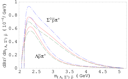
Figure 2: $d{\mathcal{B}}/dm_{\Sigma^{0}\bar{p}}$ (upper three lines) and $d{\mathcal{B}}/dm_{\Lambda\bar{p}}$ (lower three lines) plots for $\tilde{f}_{2}=\tilde{d}_{2}=\tilde{z}/2$. Dashed, solid and dot-dashed lines are for $N_{c}=2,\ 3,\ \infty$, respectively.

The axial contribution to $\Lambda(\Sigma^{0})\bar{p}\pi^{+}$ mode in the second row is about four (two) times larger than that in the first row. We find ${\mathcal{B}}(\Lambda(\Sigma^{0})\bar{p}\pi^{+})\sim[0.5\,(0.9)]\times 10^{-6}$, giving a larger rate for the $\Sigma^{0}\bar{p}\pi^{+}$ mode. These rates are similar to those obtained in Cheng:2001tr .

We show in Fig. 2 the $d{\mathcal{B}}/dm_{\Lambda\bar{p}}$ and the $d{\mathcal{B}}/dm_{\Sigma^{0}\bar{p}}$ for the $\tilde{f}_{2}=\tilde{d}_{2}=\tilde{z}/2$ case, which gives larger rates. One clearly sees threshold enhancement, which can be seen as a consequence of the need for large-$t$ suppression of the baryon form factors.

Motivated by large $\phi_{3}$ (or $\gamma$) hints He:1999mn , we show the $\phi_{3}$-dependence of the branching fractions for $\tilde{f}_{2}=\tilde{d}_{2}=\tilde{z}/2$ in Fig. 3. The larger rates for larger $\phi_{3}$ come from tree-penguin interference as in the $K^{-}\pi^{+}$ case He:1999mn .

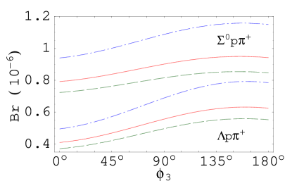
Figure 3: $\phi_{3}$-dependence of the branching fractions of $\overline{B}^{0}\to\Lambda\bar{p}\pi^{+}$ (lower three lines) and $\Sigma^{0}\bar{p}\pi^{+}$ (upper three lines) for $\tilde{f}_{2}=\tilde{d}_{2}=\tilde{z}/2$. Notation the same as Fig. 2.

IV.2 $B\to p\bar{p}\pi,\,p\bar{p}K$

Unlike the $\overline{B}^{0}\to\Lambda(\Sigma^{0})\bar{p}\pi^{+}$ case, the decay amplitude of $B^{-}\to p\bar{p}h^{-}$ with $h=\pi$ or $K$ contains both the current-produced (${\cal J}$) and transition (${\cal T}$) contributions:

$${\cal M}(p\bar{p}h^{-})={\cal J}(p\bar{p}h^{-})+{\cal T}(p\bar{p}h^{-})\,,$$ (22)

where

$${\cal J}(p\bar{p}h^{-}) = \frac{G_{F}}{\sqrt{2}}\Biggl{\{}\langle h^{-}|(\bar{q}b)_{V-A}|B^{-}\rangle$$ (23)

$$\times\biggl{\langle}p\bar{p}\,\biggl{|}V_{ub}V_{uq}^{*}\,a_{2}\,\left(\bar{u}u\right)_{V-A}-V_{tb}V_{tq}^{*}\biggl{[}a_{3}\left(\bar{u}u+\bar{d}d+\bar{s}s\right)_{V-A}+a_{4}\left(\bar{q}q\right)_{V-A}$$

$$+a_{5}\left(\bar{u}u+\bar{d}d+\bar{s}s\right)_{V+A}+\frac{3}{2}\,a_{9}\,\left(e_{u}\bar{u}u+e_{d}\bar{d}d+e_{s}\bar{s}s\right)_{V-A}\biggr{]}\biggr{|}0\biggr{\rangle}$$

$$+2a_{6}V_{tb}V_{tq}^{*}\langle h^{-}|(\bar{q}b)_{S-P}|B^{-}\rangle\langle p\bar{p}\,|\left(\bar{q}q\right)_{S+P}|0\rangle\Biggr{\}}\,,$$

with $q=d$ or $s$ for $h=\pi$ or $K$, and, from Eq. (1),

$${\cal T}(p\bar{p}h^{-}) = \frac{G_{F}}{\sqrt{2}}\bigg{\{}(V_{ub}V_{uq}^{*}a_{1}-V_{tb}V_{tq}^{*}a_{4})\langle h^{-}|(\bar{q}u)_{V-A}|0\rangle\langle p\bar{p}\,|(\bar{u}b)_{V-A}|B^{-}\rangle$$ (24)

$$-2a_{6}V_{tb}V_{tq}^{*}\frac{m^{2}_{h}}{m_{b}(m_{u}+m_{q})}\langle h^{-}|(\bar{q}u)_{V-A}|0\rangle\langle p\bar{p}\,|(\bar{u}b)_{V+A}|B^{-}\rangle\bigg{\}}$$

$$= i\,\frac{G_{F}}{\sqrt{2}}f_{h}\,m_{b}\biggl{[}\alpha_{h}\langle p\bar{p}\,|\bar{u}b|B^{-}\rangle+\beta_{h}\langle p\bar{p}\,|\bar{u}\gamma_{5}b|B^{-}\rangle\biggr{]},$$

where

$$\alpha_{h},\ \beta_{h}\equiv\left[V_{ub}V_{uq}^{*}\,a_{1}-V_{tb}V_{tq}^{*}\left(a_{4}\pm a_{6}\,\frac{2\,m_{h}^{2}}{m_{b}(m_{q}+m_{u})}\right)\right]\,.$$ (25)

It is of interest to compare the above equations with the familiar two-meson decay amplitudes Ali:1998eb . For the $B\to p\bar{p}$ transition part, the analogous transitions are $B^{-}\to\pi^{0},\,\rho^{0}$ (or the isospin-related $\overline{B}{}^{0}\to\pi^{+},\,\rho^{+}$). To single out this effect, we can search for two-meson decay modes dominated by such transitions. For the $\overline{B}{}^{0}\to\pi^{+},\,\rho^{+}$ transition dominated modes, we have $\overline{B}{}^{0}\to\pi^{+}\pi^{-}(K^{-})$ and $\overline{B}{}^{0}\to\rho^{+}\pi^{-}(K^{-})$ having decay amplitude proportional to $\alpha_{\pi(K)}$ and $\beta_{\pi(K)}$, respectively. For the $B^{-}\to\pi^{0},\,\rho^{0}$ transitions, we can find $\alpha_{K}$, $\beta_{\pi(K)}$ in $B^{-}\to\pi^{0}K^{-},\,\rho^{0}\pi^{-}(K^{-})$ decay amplitudes, respectively. The $\pi^{0}\pi^{-}$ mode is different due to the cancellation of strong penguin in $B^{-}\to\pi^{0}$ and $B^{-}\to\pi^{-}$ transition parts as they are related by isospin.

For the current-produced part, we can find similar terms in $B^{-}\to\pi^{0}\pi^{-}$, $\pi^{0}K^{-}$, $\rho^{0}\pi^{-}$ and $\rho^{0}K^{-}$ decay amplitudes. However, we have additional terms. The matrix element of the isosinglet currents $\langle p\bar{p}|(\bar{u}u+\bar{d}d+\bar{s}s)_{V,A}|0\rangle$ is non-vanishing, in contrast to the two-body $K^{-}\pi^{0}(\rho^{0})$ and $\pi^{-}\pi^{0}(\rho^{0})$ cases, where $\pi^{0}(\rho^{0})$, as a member of an isotriplet, cannot be produced via the isosinglet current. As we will see, $\langle p\bar{p}|(\bar{u}u+\bar{d}d+\bar{s}s)_{V,A}|0\rangle$ give non-negligible contributions to the $p\bar{p}K^{-}(\overline{K}{}^{0})$ modes.

IV.2.1 $B^{-}\to p\bar{p}\pi^{-}$

Although we have both current-produced and transition contributions to the $p\bar{p}\pi^{-}$ mode, the former is expected to be small due to color-suppression of the $a_{2}$ tree contribution and the smallness of CKM-suppressed penguin contributions, as one can see from Eq. (23). We show in Table 5(a) the contribution from the current-produced part ${\mathcal{J}}(p\bar{p}\pi^{-})$. As in the previous section, we are interested in the $N_{c}=3$ case and list other $N_{c}$ cases for estimation of non-factorizable effects. For $N_{c}=3$ the main contribution is from the strong penguin terms ($a_{4}$, $a_{6}$), while the tree contribution is small due to the smallness of $a_{2}$. For $N_{c}=2,\infty$, we have larger $a_{2}$ and the main contributions come form the tree amplitude. With or without non-factorizable parts, the current-produced contribution is indeed much smaller than the experimental rate ${\cal B}\left(p\bar{p}\pi^{-}\right)=\left(1.9^{+1.0}_{-0.9}\pm 0.3\right)\times 10^{-6}$ Abe:2002ds .

Table 5: (a) Current-produced ${\mathcal{B}}_{\mathcal{J}}(B^{-}\to p\bar{p}\pi^{-})$ in units of $10^{-6}$, and (b) strength of transition coefficients $C_{A,P,V5}$ giving rise to ${\mathcal{B}}_{{\mathcal{T}}}(B^{-}\to p\bar{p}\pi^{-})=1.9\times 10^{-6}$.

(a) ${\cal B}_{{\cal J}}(p\bar{p}\pi^{-})$ for $\phi_{3}=54.8^{\circ}~{}(90^{\circ})$ in units of $10^{-6}$
	$N_{c}=2$		$N_{c}=3$		$N_{c}=\infty$
	${\mathcal{B}}_{V}$	${\mathcal{B}}_{A}$	${\mathcal{B}}_{V}$	${\mathcal{B}}_{A}$	${\mathcal{B}}_{V}$	${\mathcal{B}}_{A}$
$G_{M}^{p,n}$	$0.03~{}(0.05)$	$0.03~{}(0.03)$	$0.02~{}(0.03)$	$0.01~{}(0.01)$	$0.03~{}(0.03)$	$0.09~{}(0.12)$
$F_{V},D_{V},S_{V}$	$0.05~{}(0.04)$	—	$0.00~{}(0.00)$	—	$0.15~{}(0.10)$	—
$F_{A},D_{A},S_{A}$	—	$0.09~{}(0.09)$	—	$0.02~{}(0.03)$	—	$0.29~{}(0.36)$

(b) $|C_{X}|$ values for $\phi_{3}=54.8^{\circ}~{}(90^{\circ})$ giving ${\mathcal{B}}_{{\mathcal{T}}}=1.9\times 10^{-6}$
	$N_{c}=2$	$N_{c}=3$	$N_{c}=\infty$
$|C_{A}|$ (GeV5)	56.61 (63.52)	53.28 (59.86)	47.66 (53.66)
$|C_{P}|$ (GeV8)	1233 (1356)	1160 (1278)	1038 (1146)
$|C_{V5}|$ (GeV5)	57.53 (57.53)	54.11 (54.26)	48.36 (48.77)

Since the current-produced part gives small contribution and the transition part ${\cal T}$ is governed by $a_{1}$, we expect the latter to give major contribution in the $p\bar{p}\pi$ rate. The transition part ${\cal T}$ involves unknown $B^{-}\to p\bar{p}$ transition form factors $F_{A,P,V5}$ in the matrix elements $\langle p\bar{p}|(\bar{u}b)_{S,P}|B^{-}\rangle$. We illustrate with three cases where only one form factors dominates. In each case we fit the coefficient $C_{A}$, $C_{P}$ or $C_{V5}$ to the central value of the experimental measured $p\bar{p}\pi^{-}$ rate. Note that the matrix elements $\langle p\bar{p}|(\bar{u}b)_{S,P}|B^{-}\rangle$ in Eq. (24) have nothing to do with the factorized meson $h$, hence the obtained coefficients $C_{A,P,V5}$ can be applied to the $p\bar{p}K^{-}$ mode (and for the $p\bar{p}\overline{K}{}^{0}$ mode through Eq. (18)) as well.

Table 5(b) shows the obtained values of these coefficients. It is interesting to observe that $C_{A,V5}\sim\left(m_{B}/2\right)^{5}$ and $C_{P}\sim\left(m_{B}/2\right)^{8}$. Note that the effect of $F_{A}$ and $F_{V5}$ in the $p\bar{p}\pi$ decay rate are similar. For $\phi_{3}=54.8^{\circ}\,(90^{\circ})$, we have $|\alpha_{\pi}|\sim(0.9)\,|\beta_{\pi}|$ for the color allowed tree-dominated part, leading to $|C_{A}|\sim(1.1)\,|C_{V5}|$. Unlike the current-produced part, the transition part is not sensitive to $N_{c}$, since $\alpha_{\pi}$, $\beta_{\pi}$ (composed of $a_{1}$, $a_{4}$ and $a_{6}$) do not depend strongly on $N_{c}$ as $a_{2}$.

Table 6: ${\cal B}(B^{-}\to p\bar{p}\pi^{-})$ in units of $10^{-6}$ for $\phi_{3}=54.8^{\circ}~{}(90^{\circ})$ with $\tilde{f}_{2}=\tilde{d}_{2}=\tilde{z}/2$, $s_{2}=\tilde{s}_{2}=0$.

	$N_{c}=2$		$N_{c}=3$		$N_{c}=\infty$
	$+|C_{X}|$	$-|C_{X}|$	$+|C_{X}|$	$-|C_{X}|$	$+|C_{X}|$	$-|C_{X}|$
$X=A$	$2.24~{}(2.42)$	$1.84~{}(1.66)$	$1.88~{}(2.07)$	$1.96~{}(1.79)$	$1.83~{}(2.01)$	$2.85~{}(2.70)$
$X=P$	$1.99~{}(2.15)$	$2.10~{}(1.92)$	$1.86~{}(2.06)$	$1.97~{}(1.80)$	$2.29~{}(2.50)$	$2.39~{}(2.20)$
$X=V5$	$2.62~{}(2.55)$	$1.47~{}(1.53)$	$1.99~{}(2.03)$	$1.85~{}(1.82)$	$1.41~{}(1.64)$	$3.27~{}(3.06)$

By combining the transition contributions with the current-produced part for $\tilde{f}_{2}=\tilde{d}_{2}=\tilde{z}/2$, $s_{2}=\tilde{s}_{2}=0$ case, we obtain the total branching fractions shown in Table 6. We see that the rates are still similar to the experimental central value, justifying our procedure.

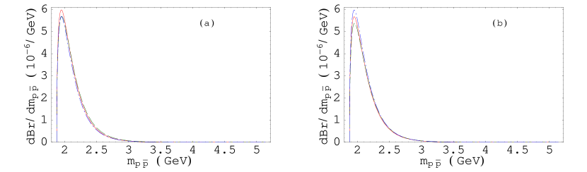
Figure 4: $d{\mathcal{B}}/d\,m_{p\bar{p}}$ spectrum for the $B^{-}\to p\bar{p}\pi^{-}$ mode with $N_{c}=3$ and $\phi_{3}=54.8^{\circ}$. Solid, dash and dot-dash lines in (a) and (b) correspond to $\mp|C_{V}|$, $\mp|C_{A}|$ and $\mp|C_{P}|$, respectively.

In Fig. 4 we plot $d{\mathcal{B}}/d\,m_{p\bar{p}}$ for the $B^{-}\to p\bar{p}\pi^{-}$ mode, for the $N_{c}=3$ case with $\phi_{3}=54.8^{\circ}$, $C_{A}=\mp|C_{A}|$, $C_{P}=\mp|C_{P}|$ and $C_{V5}=\mp|C_{V5}|$, respectively. It is clear that the three cases give close to identical results. The threshold enhancement phenomena is evident, as has already been shown in the $\overline{B}^{0}\to\Lambda(\Sigma^{0})p\pi^{+}$ cases. However, we have a much faster $1/m_{p\bar{p}}$ suppression here due to the $1/t^{3,4}$ behavior of the dominant transition form factors, while for the $\Lambda(\Sigma^{0})p\pi^{+}$ modes the form factors only behave as $1/t^{2}$ in the large $t$ limit. It would be interesting to verify the faster $1/m_{p\bar{p}}$ fall off experimentally.

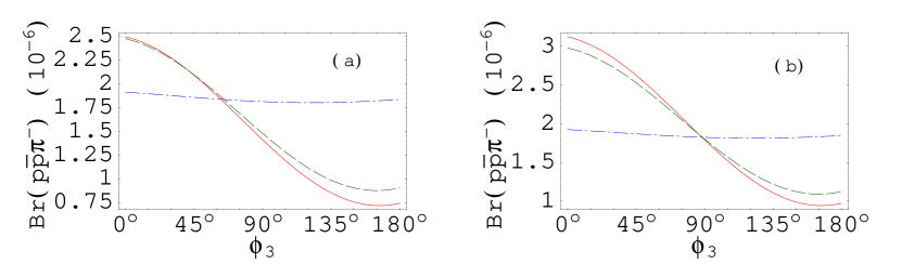
Figure 5: $\phi_{3}$-dependence of $B^{-}\to p\bar{p}\pi^{-}$ branching fraction for $\tilde{f}_{2}=\tilde{d}_{2}=\tilde{z}/2$, $s_{2}=\tilde{s}_{2}=0$ and $N_{c}=3$. Solid, dash and dot-dash lines for $-|C_{A}|$, $-|C_{P}|$ and $-|C_{V5}|$, respectively. The plots are fixed to $\phi_{3}=$ (a) $54.8^{\circ}$, (b) $90^{\circ}$ values given in Table 6.

In Fig. 5 we illustrate the $\phi_{3}$-dependence of the $p\bar{p}\pi^{-}$ branching fractions, with $\phi_{3}=54.8^{\circ}$ and $90^{\circ}$ results fixed to those of Table 6. Since this mode is dominated by the transition part, we expect similar $\phi_{3}$ behavior as in $\overline{B}{}^{0}\to\pi^{+}\pi^{-},\,\rho^{+}\pi^{-}$ decay rates. The behavior of the rates from the $C_{A}$, $C_{P}$ terms are similar to the $\pi^{+}\pi^{-}$ case He:1999mn rather than the $\pi^{-}\pi^{0}$ case. We have a similar $\alpha_{\pi}$ term in the $\pi^{+}\pi^{-}$ amplitude, while due to cancellation in the current-produced and the transition terms, there is no strong penguin in the $\pi^{-}\pi^{0}$ amplitude, resulting in small tree-penguin interference. The $C_{V5}$ case is similar to $\overline{B}{}^{0}\to\rho^{+}\pi^{-}$ and does not show strong $\phi_{3}$ dependence. As noted before, both features can be understood from the expression of $\alpha_{\pi}$ and $\beta_{\pi}$ in Eq. (25).

IV.2.2 $B^{-}\to p\bar{p}K^{-}$

Table 7: (a) Current ${\mathcal{B}}_{{\cal J}}(B^{-}\to p\bar{p}K^{-})$ and (b) transition ${\mathcal{B}}_{{\cal J}}(B^{-}\to p\bar{p}K^{-})$ in units of $10^{-6}$.

(a) ${\cal B}_{{\cal J}}(p\bar{p}K^{-})$ in units of $10^{-6}$ for $\phi_{3}=54.8^{\circ}~{}(90^{\circ})$
	$N_{c}=2$		$N_{c}=3$		$N_{c}=\infty$
	${\mathcal{B}}_{V}$	${\mathcal{B}}_{A}$	${\mathcal{B}}_{V}$	${\mathcal{B}}_{A}$	${\mathcal{B}}_{V}$	${\mathcal{B}}_{A}$
$G_{M}^{p,n}$	$0.02~{}(0.02)$	$0.10~{}(0.09)$	$0.01~{}(0.01)$	$0.06~{}(0.06)$	$0.33~{}(0.31)$	$0.01~{}(0.02)$
$F_{V},D_{V},S_{V}$	$0.65~{}(0.69)$	—	$0.26~{}(0.26)$	—	$0.02~{}(0.03)$	—
$F_{A},D_{A},S_{A}$	—	$0.23~{}(0.19)$	—	$0.12~{}(0.12)$	—	$0.02~{}(0.05)$

(b) ${\cal B}_{{\cal T}}(p\bar{p}K^{-})$ in units of $10^{-6}$ for $\phi_{3}=54.8^{\circ}~{}(90^{\circ})$
	$N_{c}=2$	$N_{c}=3$	$N_{c}=\infty$
$C_{A}\qquad$	$2.08~{}(3.42)$	$2.12~{}(3.48)$	$2.18~{}(3.58)$
$C_{P}\qquad$	$1.83~{}(2.86)$	$1.86~{}(2.91)$	$1.90~{}(2.99)$
$C_{V5}\qquad$	$0.26~{}(0.20)$	$0.23~{}(0.19)$	$0.18~{}(0.18)$

For the $B^{-}\to p\bar{p}K^{-}$ decay, we have both a transition (${\mathcal{T}}$) part and now a more effective current-produced (${\mathcal{J}}$) part, as shown in Table 7(a). For the vector part, the largest contributions come from $(a_{3}+a_{5})\langle p\bar{p}|(\bar{u}u+\bar{d}d+\bar{s}s)_{V}|0\rangle$ and $a_{4}\langle p\bar{p}|(\bar{s}s)_{V}|0\rangle$ in Eq. (23). In the first line of the table, we have $\langle p\bar{p}|(\bar{s}s)_{V,A,S,P}|0\rangle=0$ and the contributions are mainly from the $a_{3}+a_{5}$ term. For $N_{c}=3$, $a_{3}+a_{5}$ is small, resulting in a small ${\mathcal{B}}_{V}$. In the second line, the $a_{4}\langle p\bar{p}|(\bar{s}s)_{V}|0\rangle$ term gives ${\mathcal{B}_{V}}\sim 0.3\times 10^{-6}$ and interferes differently with the previous term for different $N_{c}$ as $a_{3}+a_{5}$ changes sign. On the other hand, the $(a_{3}-a_{5})\langle p\bar{p}|(\bar{u}u+\bar{d}d+\bar{s}s)_{A}|0\rangle$ term dominates in the axial part. The dependence on $N_{c}$ of these contributions can be understood from the behavior of $a_{3}-a_{5}$.

We now turn to the transition ($\mathcal{T}$) part. For $\phi_{3}\sim 54.8^{\circ}\,(90^{\circ})$, we have $|\alpha_{K}|\sim|\alpha_{\pi}|$ $(|\alpha_{K}|\gtrsim|\alpha_{\pi}|)$ and hence ${\mathcal{B}}_{\mathcal{T}}(p\bar{p}K^{-})\sim({\rm or\ }\gtrsim)\ {\mathcal{B}}_{\mathcal{T}}(p\bar{p}\pi^{-})$ from the $C_{A,P}$ contributions. On the other hand, $a_{4}$ and $a_{6}$ in $\beta_{K}$ are partially canceled and the tree contribution is CKM suppressed, resulting in $|\beta_{K}|^{2}\ll|\alpha_{K}|^{2}$. Hence, the $\langle p\bar{p}|\bar{u}b|B^{-}\rangle$ contribution containing $C_{A,P}$ is much larger than the $\langle p\bar{p}|\bar{u}\gamma_{5}b|B^{-}\rangle$ case coming from $C_{V5}$, as can be seen from Table 7(b). Note further that the $\phi_{3}=90^{\circ}$ case from $C_{A,P}$ gives larger rates, as should be expected from the analogous $K^{+}\pi^{-}$ mode He:1999mn .

We combine the current-produced contribution with the transition part and give the total branching fractions in Table 8. The results prefer the $\phi_{3}=90^{\circ}$ case. Numbers shown in the first two lines of Table 8 are close to the the experimental rate ${\cal B}(B^{\pm}\to p\bar{p}K^{\pm})=(4.3^{+1.1}_{-0.9}\pm 0.5)\times 10^{-6}$ Abe:2002ds . We see that, for the $\phi_{3}=90^{\circ}$, $N_{c}=3$ and $C_{A}=-|C_{A}|$ case we have ${\mathcal{B}}=4.26\times 10^{-6}$, which is closest to the central value of the experimental rate. The value only changes by 10% as we modify $N_{c}$ to $2$ or $\infty$.

Table 8: ${\cal B}(B^{-}\to p\bar{p}K^{-})$ in units of $10^{-6}$ for $\phi_{3}=54.8^{\circ}~{}(90^{\circ})$, with $\tilde{f}_{2}=\tilde{d}_{2}=\tilde{z}/2$, $s_{2}=\tilde{s}_{2}=0$.

	$N_{c}=2$		$N_{c}=3$		$N_{c}=\infty$
	$+|C_{X}|$	$-|C_{X}|$	$+|C_{X}|$	$-|C_{X}|$	$+|C_{X}|$	$-|C_{X}|$
$X=A$	$2.56~{}(3.85)$	$3.36~{}(4.75)$	$2.18~{}(3.45)$	$2.82~{}(4.26)$	$2.06~{}(3.36)$	$2.38~{}(3.96)$
$X=P$	$2.72~{}(3.75)$	$2.70~{}(3.73)$	$2.25~{}(3.30)$	$2.23~{}(3.28)$	$1.95~{}(3.08)$	$1.94~{}(3.07)$
$X=V5$	$0.83~{}(1.08)$	$1.45~{}(1.08)$	$0.42~{}(0.57)$	$0.80~{}(0.56)$	$0.16~{}(0.16)$	$0.28~{}(0.36)$

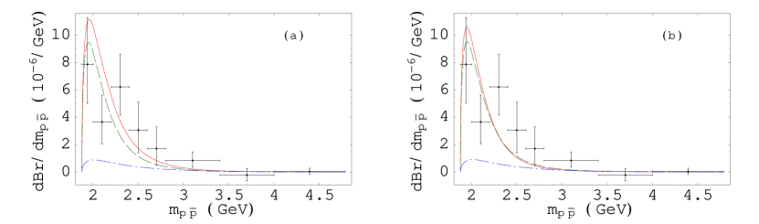
Figure 6: $d{\mathcal{B}}/d\,m_{p\bar{p}}$ of the $p\bar{p}K^{-}$ mode with $\phi_{3}=90^{\circ}$ and $N_{c}=3$. The solid, dashed and the dot-dashed lines in (a) and (b) stand for the $C_{A}=\mp|C_{A}|$, $C_{P}=\mp|C_{P}|$ and the $C_{V5}=\mp|C_{V5}|$ case, respectively.

We plot $d{\mathcal{B}}/d\,m_{p\bar{p}}$ in Fig. 6 for the $\phi_{3}=90^{\circ}$, $N_{c}=3$ case of Table 8. The curves from $C_{A}$, $C_{P}$ terms are close to data points taken from Ref. Abe:2002ds . The curve from $C_{V5}$ term is too low as expected from the smallness of $\beta_{K}$. For the first two cases, one can see that, except for a possible bump at $m_{p\bar{p}}\sim 2.2$–2.4 GeV, the behavior of the decay spectrum including threshold enhancement can be explained naturally. Comparing with Fig. 4, we note that the suppression for large $m_{p\bar{p}}$ is milder than the $p\bar{p}\pi^{-}$ case. This is due to the presence of the current-produced part which has less suppressed form factors ($1/t^{2}$), which dominates over the transition part in the large $t$ region.

We give in Fig. 7 the $\phi_{3}$-dependence of ${\mathcal{B}}(p\bar{p}K^{-})$. The $C_{A,P}$ cases are similar to the $K^{-}\pi^{+}$ mode He:1999mn , while the $C_{V5}$ case is similar to the $K^{-}\rho^{+}$ case as discussed before. We note that the experimental indication that the $p\bar{p}K^{-}$ rate is larger than the $p\bar{p}\pi^{-}$ rate seems to favor larger $\phi_{3}$ values such as $90^{\circ}$ case, analogous to $B$ to two meson decay situation He:1999mn .

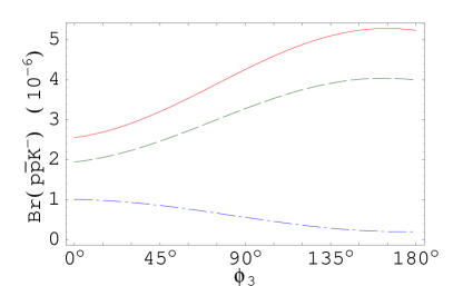
Figure 7: $\phi_{3}$-dependence of ${\cal B}(B^{-}\to p\bar{p}K^{-})$. Solid, dash and dot-dash lines stand for the $C_{A}=-|C_{A}|$, $C_{P}=-|C_{P}|$ and $C_{V5}=-|C_{V5}|$ cases, respectively.

IV.2.3 $\overline{B}^{0}\to p\bar{p}\overline{K}{}^{0}$

For the $\overline{B}^{0}\to p\bar{p}\overline{K}{}^{0}$ decay, we have ${\cal M}(p\bar{p}\overline{K}{}^{0})={\cal J}(p\bar{p}\overline{K}{}^{0})+{\mathcal{T}}(p\bar{p}\overline{K}{}^{0})$. Since $\langle\overline{K}{}^{0}|(\bar{s}b)_{V-A}|\overline{B}{}^{0}\rangle=\langle K^{-}|(\bar{s}b)_{V-A}|B^{-}\rangle$ by isospin, we have

$${\cal J}(p\bar{p}\overline{K}{}^{0})={\cal J}(p\bar{p}K^{-})\,.$$ (26)

On the other hand,

$${\cal T}(p\bar{p}\overline{K}{}^{0})=i\,\frac{G_{F}}{\sqrt{2}}f_{\overline{K}{}^{0}}\,m_{b}\biggl{[}\alpha_{\overline{K}{}^{0}}\langle p\bar{p}\,|\bar{d}b|\overline{B}{}^{0}\rangle+\beta_{\overline{K}{}^{0}}\langle p\bar{p}\,|\bar{d}\gamma_{5}b|\overline{B}{}^{0}\rangle\biggr{]},$$ (27)

with

$$\alpha_{\overline{K}{}^{0}},\ \beta_{\overline{K}{}^{0}}\equiv-V_{tb}V_{ts}^{*}\left(a_{4}\pm a_{6}\,\frac{2\,m_{\overline{K}{}^{0}}^{2}}{m_{b}(m_{s}+m_{d})}\right)\,.$$ (28)

Table 9: (a) Current ${\mathcal{B}}_{{\cal J}}(\overline{B}^{0}\to p\bar{p}\overline{K}{}^{0})$ and (b) transition ${\mathcal{B}}_{{\cal T}}(\overline{B}^{0}\to p\bar{p}\overline{K}{}^{0})$ in units of $10^{-6}$.

(a) ${\cal B}_{{\cal J}}(p\bar{p}\overline{K}^{0})$ in units of $10^{-6}$ for $\phi_{3}=54.8^{\circ}~{}(90^{\circ})$.
	$N_{c}=2$		$N_{c}=3$		$N_{c}=\infty$
	${\mathcal{B}}_{V}$	${\mathcal{B}}_{A}$	${\mathcal{B}}_{V}$	${\mathcal{B}}_{A}$	${\mathcal{B}}_{V}$	${\mathcal{B}}_{A}$
$G_{M}^{p,n}$	$0.02~{}(0.02)$	$0.10~{}(0.08)$	$0.01~{}(0.01)$	$0.06~{}(0.05)$	$0.31~{}(0.29)$	$0.01~{}(0.02)$
$F_{V},D_{V},S_{V}$	$0.61~{}(0.65)$	—	$0.25~{}(0.24)$	—	$0.02~{}(0.03)$	—
$F_{A},D_{A},S_{A}$	—	$0.21~{}(0.18)$	—	$0.12~{}(0.11)$	—	$0.02~{}(0.05)$

(b) ${\cal B}_{{\cal T}}(p\bar{p}\overline{K}{}^{0})$ in units of $10^{-6}$ for $\phi_{3}=54.8^{\circ}~{}(90^{\circ})$.
	$N_{c}=2$	$N_{c}=3$	$N_{c}=\infty$
$C_{A}\qquad$	$2.74~{}(3.37)$	$2.78~{}(3.43)$	$2.84~{}(3.52)$
$C_{P}\qquad$	$0.12~{}(0.14)$	$0.12~{}(0.15)$	$0.13~{}(0.15)$
$C_{V5}\qquad$	$1.91~{}(1.87)$	$1.93~{}(1.89)$	$1.96~{}(1.95)$

We show in Table 9 the separate current-produced and transition contributions to the $p\bar{p}\overline{K}{}^{0}$ decay rate. As explained in the above, the current-produced part is identical to the $p\bar{p}K^{-}$ case, except for the difference in $\tau_{B^{-}}$ and $\tau_{B^{0}}$. For the transition part, the transition form factors are related to the $p\bar{p}K^{-}$ case through Eq. (18). We concentrate on the $(\bar{d}b)_{S}$ form factors instead of $(\bar{d}b)_{P}$, since $|\alpha_{\overline{K}{}^{0}}|\gg|\beta_{\overline{K}{}^{0}}|$. We have ${\cal F}_{A}=1.1F_{A}+0.9F_{V5}$ and ${\cal F}_{P}=-F_{P}/4$ for the $(\bar{d}b)_{S}$ form factors. Since ${\cal F}^{p\bar{p}\overline{K}{}^{0}}_{P}/{\cal F}^{p\bar{p}K^{-}}_{P}=-1/4$, the contribution form the $C_{P}$ term is very small. The ratio of the $C_{A}$ and $C_{V5}$ contributions can be understood as well. For $\phi_{3}=54.8^{\circ}$, the $F_{A}$ dominated case is larger than the $F_{V5}$ dominated case by a factor of $11/9$ in amplitude, giving a rate enhancement $\sim(11/9)^{2}|C_{A}/C_{V5}|^{2}\sim(11/9)^{2}\sim 1.5$. For $\phi_{3}=90^{\circ}$, we have a further 10% growth in amplitude due to $|C_{A}|\sim 1.1|C_{V5}|$ (as shown in Table 5(b)), and the rate enhancement becomes $\sim 1.8$. It is interesting to compare the transition contributions to those in the $p\bar{p}K^{-}$ mode: for the $C_{A}$ dominated case, ${\mathcal{B}}_{\mathcal{T}}(p\bar{p}\overline{K}{}^{0})\sim{\mathcal{B}}_{\mathcal{T}}(p\bar{p}K^{-})$; for the $C_{P}$ dominated case, ${\mathcal{B}}_{\mathcal{T}}(p\bar{p}\overline{K}{}^{0})\ll{\mathcal{B}}_{\mathcal{T}}(p\bar{p}K^{-})$; for the $C_{V5}$ dominated case, ${\mathcal{B}}_{\mathcal{T}}(p\bar{p}\overline{K}{}^{0})\gg{\mathcal{B}}_{\mathcal{T}}(p\bar{p}K^{-})$.

We give in Table 10 the full branching fraction by combining the current-produced and transition parts in amplitude. For the $N_{c}=3$, $\phi_{3}=54.8^{\circ}\,[90^{\circ}]$ case, we have ${\mathcal{B}}(p\bar{p}\overline{K}{}^{0})=(0.5$–$3.6)\times 10^{-6}$ [(0.5–$4.3)\times 10^{-6}$]. It could be close to or smaller than the $p\bar{p}K^{-}$ rate.

In Fig. 8 we plot $d{\mathcal{B}}/d\,m_{p\bar{p}}$ for the $\overline{B}^{0}\to p\bar{p}\overline{K}{}^{0}$ mode. The decay spectrum for the $C_{A}$ and $C_{V5}$ cases are similar to the $C_{A}$, $C_{P}$ cases in the $p\bar{p}K^{-}$ mode. They exhibit threshold enhancement and a slower fall off for large $t$ compared to the $p\bar{p}\pi^{-}$ case. For the $C_{A}$ case, where the rate is not far from $p\bar{p}K^{-}$, the decay spectrum could be checked soon.

Table 10: ${\cal B}(B^{-}\to p\bar{p}\overline{K}{}^{0})$ in units of $10^{-6}$, for $\phi_{3}=54.8^{\circ}~{}(90^{\circ})$ and $\tilde{f}_{2}=\tilde{d}_{2}=\tilde{z}/2$, $s_{2}=\tilde{s}_{2}=0$.

	$N_{c}=2$		$N_{c}=3$		$N_{c}=\infty$
	$+|C_{X}|$	$-|C_{X}|$	$+|C_{X}|$	$-|C_{X}|$	$+|C_{X}|$	$-|C_{X}|$
$X=A$	$2.91~{}(3.53)$	$4.21~{}(4.86)$	$2.68~{}(3.28)$	$3.60~{}(4.28)$	$2.71~{}(3.32)$	$3.05~{}(3.88)$
$X=P$	$0.95~{}(0.97)$	$0.94~{}(0.96)$	$0.48~{}(0.50)$	$0.48~{}(0.49)$	$0.17~{}(0.23)$	$0.16~{}(0.22)$
$X=V5$	$2.13~{}(2.14)$	$3.33~{}(3.25)$	$1.88~{}(1.85)$	$2.70~{}(2.64)$	$1.86~{}(1.82)$	$2.14~{}(2.24)$

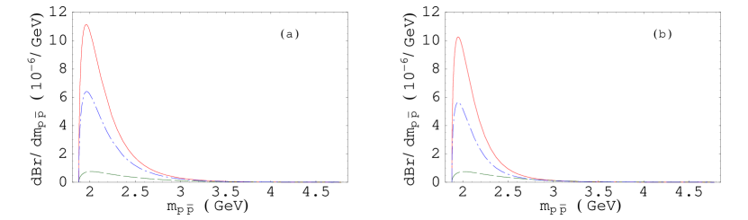
Figure 8: $d{\mathcal{B}}/d\,m_{p\bar{p}}$ for the $\overline{B}^{0}\to p\bar{p}\overline{K}{}^{0}$ mode with $\tilde{f}_{2}=\tilde{d}_{2}=\tilde{z}/2$, $s_{2}=\tilde{s}_{2}$. Solid, dash and dot-dash lines in (a) and (b) are for $C_{A}=\mp|C_{A}|$, $C_{P}=\mp|C_{P}|$ and $C_{V5}=\mp|C_{V5}|$ cases, respectively.

In Fig. 9 we show the $\phi_{3}$-dependence of ${\mathcal{B}}(p\bar{p}\overline{K}{}^{0})$. As shown in Eq. (28), the transition part does not have tree-penguin interference and hence the mild $\phi_{3}$ dependence is from the sub-dominant current-produced term.

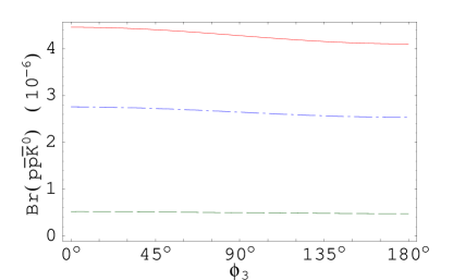
Figure 9: $\phi_{3}$-dependence of ${\cal B}(\overline{B}^{0}\to p\bar{p}\overline{K}{}^{0})$ for $\tilde{f}_{2}=\tilde{d}_{2}=\tilde{z}/2$, $s_{2}=\tilde{s}_{2}=0$. Solid, dash and dot-dash lines are for $C_{A}=-|C_{A}|$, $C_{P}=-|C_{P}|$ and $C_{V5}=-|C_{V5}|$ cases, respectively.

IV.3 Comparison with Other Works

Before we end this section, we compare our work with some others. There are approaches that use pole models to evaluate decay matrix elements. For example, Ref. Piccinini use $K^{*}$ pole for $\bar{\Lambda}p$ production in $B\to\eta^{\prime}\Lambda p$ decay, while Ref. Cheng:2001tr use pole models in two-body and three-body baryonic B decay. We focus on the comparison with the Ref. Cheng:2001tr as we have some subjects in common.

In Ref. Cheng:2001tr , Cheng and Yang use a factorization approach in the current-produced ($\mathcal{J}$) amplitude. Their approach is similar to ours (up to some technical differences), hence they obtain results similar to ours in current production dominated modes, such as $\bar{B}^{0}\to\Lambda\bar{p}\pi^{+}$, $\Sigma^{0}\bar{p}\pi^{+}$. However, there is considerable difference in the transition ($\mathcal{T}$) part. We factorize the amplitude into a current-produced meson and a $B$ to baryonic pair transition amplitude. In their approach, they use a simple pole model to evaluate this part. For example, in $B^{-}\to p\bar{p}K^{-}$ decay, they have a strong process $B^{-}\to\{\Lambda^{(*)}_{b},\Sigma^{0(*)}_{b}\}\bar{p}$, followed by a weak $\{\Lambda^{(*)}_{b},\Sigma^{0(*)}_{b}\}\to pK^{-}$ decay. From their modeling of the strong coupling $g_{\Lambda_{b}\to B^{-}p}=3\sqrt{3}g_{\Sigma^{0}_{b}\to B^{-}p}$, they can give $p\bar{p}K^{-}$ rate that is close to experimental result by using monopole $q^{2}$ dependence of $g_{\Lambda_{b}\to B^{-}p}$. The $m_{p\bar{p}}$ spectrum given in Ref. Cheng:2001tr shows a peak around $t\sim 6\,{\rm GeV}^{2}$ (or $m_{p\bar{p}}\sim 2.5$ GeV), while we have a sharper peak in lower $m_{p\bar{p}}$ (around 2 GeV). The difference is due to the $1/t^{3}$ behavior in our transition part from QCD counting rule, while they have $\sim 1/t^{2}$ from the pole model. On the other hand, one expects peaking behavior towards large $m_{pK^{-}}$ due to $\Lambda_{b}$ pole in their approach, while in this work we do not expect any structure (since $K^{-}$ and $p$ are factorized) in the $m_{pK^{-}}$ spectrum. In turn, they expect $p\bar{p}\overline{K}{}^{0}$ rate $\sim 10^{-7}$ due to the absence of $\Lambda_{b}$ pole, while we expect a rate that could be as large as $p\bar{p}K^{-}$, although $10^{-7}$ is also possible. It is up to experiment to check the $m_{pK^{-}}$ spectrum and the $p\bar{p}\overline{K}{}^{0}$ rate.

We recall that in Ref. Chua:2001vh we also tried a VMD (dispersion analysis) approach Hammer:1996kx ; Mergell:1996bf in the current production dominated $B^{0}\to D^{*-}p\bar{n}$ decay. In this approach, the strong coupling for each pole is fixed at the pole mass, hence each pole gives a monopole contribution to the total form factors. One needs to have more than one pole with cancellations in order to reproduce the correct QCD counting rule, which is $1/t^{2}$ for current-produced form factors Hammer:1996kx ; Mergell:1996bf . We likely would have the same situation here, that more than one pole is needed to reproduced the large $t$ behavior. If we take a multi-pole approach, the baryonic transition form factor can be expressed as $B\to M_{i}$ transitions with $M_{i}$ as one of the mesons, followed by a strong process $M_{i}\to{\bf B\overline{B}^{\prime}}$ (similar to Ref. Piccinini ). Summing over $i$, the QCD counting rule should be taken as a constraint. Instead of doing so, in part because of lack of independent data, we use a simplified transition form factor motivated from the QCD counting rule directly in this work, and wait for experimental data, such as semi-leptonic $B\to{\bf B\bar{B}^{\prime}}l\nu$ and semi-inclusive $B\to{\bf B\bar{B}^{\prime}}X$ (similar to $B\to\pi X$ He:2002ae ), to improve our understanding. One may resort to the multi-pole approach once these measurements become available.

V Discussion and Conclusion

In this work we use factorization approach to study charmless three-body baryonic $B$ decays. We apply SU(3) relations and QCD counting rules on baryon form factors. We identify two mechanisms of baryon pair production, namely current-produced and transition. The $\Sigma^{0}\bar{p}\pi^{+}$ and $\Lambda\bar{p}\pi^{+}$ modes arise solely from the current-produced part, with rates of order $10^{-7}-10^{-6}$. The $p\bar{p}\pi^{-}$, $p\bar{p}K^{-}$ and $p\bar{p}\overline{K}{}^{0}$ modes are dominated by transition contributions, while the current-produced contributions in the last two cases are significant.

Due to the absence of $S_{V,A}$ in the current-produced amplitude, and the complete absence of the transition amplitude, $\Sigma^{0}\bar{p}\pi^{+}$ and $\Lambda\bar{p}\pi^{+}$ modes are the simplest in this work. However, they are sensitive to how we treat the chiral limit of the pseudoscalar term (which has an $a_{6}$ coefficient). On the other hand, we neglect $F_{2}$ contribution in the vector part. It remains to be checked whether this is a good approximation or not. It may in turn give us information on $F_{2}$, or equivalently $G_{E}$, from these measurements. In particular, the vector current form factors in $\Lambda\bar{p}\pi^{+}$ are only related to the proton $G_{M,E}$ from SU(3) symmetry (as one can see from Eq. (21) and Table 3), and we may obtain information of $G_{E}^{p}$ from this mode.

The $\phi_{3}$ dependence of $\Lambda\bar{p}\pi^{+}$, $\Sigma^{0}\bar{p}\pi^{+}$ rates are similar to $K^{-}\pi^{+}$, $K^{*-}\pi^{+}$ modes. Since transition contributions dominate in the $p\bar{p}h$ modes, the $\phi_{3}$ dependence of $p\bar{p}\pi^{-}(K^{-})$ rate is similar to that in the two-body $\overline{B}{}^{0}\to\pi^{+}\pi^{-}(K^{-})$ or $\rho^{+}\pi^{-}(K^{-})$ decays, while the $\phi_{3}$ dependence of $p\bar{p}\overline{K}{}^{0}$ rate is mild.

Under factorization, the $p\bar{p}\pi^{-}$ and the $p\bar{p}K^{-}$ modes have the same baryonic transition form factors. Since the $p\bar{p}\pi^{-}$ mode is dominated by baryonic transition contribution, we use it to fit for the transition form factor parameters and apply them to the $p\bar{p}K^{-}$ case. To keep $p\bar{p}\pi^{-}$ rate around the experimental central value but allowing $p\bar{p}K^{-}$ rate to be larger, data seems to favor a larger $\phi_{3}$. The $p\bar{p}\overline{K}{}^{0}$ rate can be similar to or much smaller than the $p\bar{p}K^{-}$ rate. We do not consider modes involving vector mesons, such as $p\bar{p}K^{*}$, since they will involve further unknown form factors.

It is interesting that we can reproduce $p\bar{p}K^{-}$ decay spectrum based on QCD counting rules, indicating that the latter is a rather robust theoretical tool. From QCD counting rules, the current-produced baryonic form factors behave like $1/t^{2}$, while the transition baryonic form factors behave like $1/t^{3}$ in large $t\ (\equiv m^{2}_{\rm\bf BB^{\prime}})$ limit. The $p\bar{p}\pi^{-}$ decay is dominated by the transition part and hence shows a faster damping behavior for large $t$. In contrast, the $\Lambda\bar{p}\pi^{+}$, $\Sigma^{0}\bar{p}\pi^{+}$, $p\bar{p}K^{-}$ and $p\bar{p}\overline{K}{}^{0}$ modes contain current-produced part, and show a slower damping behavior for large $t$. We expect an even slower damping behavior (form factors $\sim 1/t$) in three-body mesonic $B$ decay. These can be checked soon, especially by comparing the $p\bar{p}K^{-}$ and the $p\bar{p}\pi^{-}$ spectra.

We note that there is a possible bump around $m_{p\bar{p}}=2.3$ GeV in the $p\bar{p}K^{-}$ decay spectrum. It is interesting that the position is close to the mass of a glueball candidate $\xi(2230)$, also known as $f_{J}(2220)$, with $m=2231\pm 3.5$ MeV and $\Gamma=23^{+8}_{-7}$ MeV Groom:in . Combining ${\mathcal{B}}(J/\psi\to\gamma\xi)\gtrsim 2.5\times 10^{-3}$ Groom:in and ${\mathcal{B}}(J/\psi\to\gamma\xi)\,{\mathcal{B}}(\xi\to p\bar{p})=(1.5^{+0.6}_{-0.5}\pm 0.5)\times 10^{-5}$ Bai:wm , we have ${\mathcal{B}}(\xi\to p\bar{p})\lesssim 6\times 10^{-3}$. If the rate in the whole $2.2<M_{p\bar{p}}<2.4$ GeV bin is due to this resonance, we would have ${\mathcal{B}}(B^{-}\to K^{-}\xi)\,{\mathcal{B}}(\xi\to p\bar{p})\sim 1.24\times 10^{-6}$. We thus get ${\mathcal{B}}(B^{-}\to K^{-}\xi)\gtrsim 2\times 10^{-4}$, or a few times the rate of ${\mathcal{B}}(B^{-}\to\eta^{\prime}K^{-})=(6.5\pm 1.7)\times 10^{-5}$ Groom:in . Since both $\xi$ and $\eta^{\prime}$ are glue rich hadrons, while $b\to s$ decays provide glue rich environment Atwood:1997de , this may be of great interest. The underlying dynamics could be $g^{*}\to g\xi$, which is analogous to $g^{*}\to g\eta^{\prime}$ for $B\to\eta^{\prime}+X_{s}$ decay Atwood:1997bn . One should also search in three-body mesonic decay modes. However, as noted, a slower fall off for non-resonance part, together with interference with possible nearby resonances, may produce physical background. But $B\to p\bar{p}K^{-}$ decay could be a rather clean mode to search for $\xi$ xi .

Appendix A Some useful Formulas

In general, for a three-body decay $B\to h{\rm\bf B}\overline{\rm\bf B}^{\prime}$, the amplitude can always be written in the following form:

$${\cal M}\left(B\to h{\rm\bf B}\overline{\rm\bf B}^{\prime}\right) = \frac{G_{F}}{\sqrt{2}}\,\biggl{\{}{\cal A}\,\bar{u}(p_{{\mathbf{B}}})\,/\!\!\!p_{h}v(p_{\overline{\mathbf{B}}^{\prime}})+{\mathcal{B}}\,\bar{u}(p_{{\mathbf{B}}})\,/\!\!\!p_{h}\gamma_{5}v(p_{\overline{\mathbf{B}}^{\prime}})$$ (29)

$$\qquad\qquad+\,{\cal C}\,\bar{u}(p_{{\mathbf{B}}})\gamma_{5}v(p_{\overline{\mathbf{B}}^{\prime}})+{\cal D}\,\bar{u}(p_{{\mathbf{B}}})v(p_{\overline{\mathbf{B}}^{\prime}})\biggr{\}}\,,$$

whose absolute square is given by

$$\Sigma\,\left|{\cal M}\right|^{2} = G_{F}^{2}\,\Biggl{\{}\left|{\cal A}\right|^{2}\biggl{[}\Bigl{(}m_{B}^{2}+m_{2}^{2}-m_{12}^{2}-m_{23}^{2}\Bigr{)}\,\Bigl{(}m_{23}^{2}-m_{2}^{2}-m_{3}^{2}\Bigr{)}$$ (30)

$$\qquad\qquad\qquad\qquad\qquad\qquad\qquad\quad-m_{3}^{2}\,\Bigl{(}m_{12}^{2}-(m_{1}-m_{2})^{2}\Bigr{)}\biggr{]}$$

$$+ 2\,{\rm Re}\left({\cal A}\,{\cal D}^{*}\right)\,\biggl{[}m_{1}\Bigl{(}m_{23}^{2}-m_{2}^{2}-m_{3}^{2}\Bigr{)}-m_{2}\Bigl{(}m_{B}^{2}+m_{2}^{2}-m_{12}^{2}-m_{23}^{2}\Bigr{)}\biggr{]}\Biggr{\}}$$

$$+ \left|{\cal D}\right|^{2}\,\biggl{[}m_{12}^{2}-(m_{1}+m_{2})^{2}\biggr{]}\ +\ ({\cal A}\to{\cal B},\,{\cal D}\to{\cal C},\,m_{2}\to-m_{2})\,,$$

where the summation is over all spins, and we have adopted the convention that the relatively positive baryon is assigned as particle 1, the other baryon is assigned as particle 2, the meson $h$ is always assigned as particle 3. One can see from the above that only Re$\left({\cal A}{\cal D}^{*}\right)$ and Re$\left({\cal B}{\cal C}^{*}\right)$ appear as interference terms upon squaring. Given these formulas, the task is now reduced to obtain the ${\cal A}$–${\cal D}$ terms for an amplitude of interest.

It is straightforward to obtain the decay rate $\Gamma$ from the integration of

$$d\Gamma=\frac{1}{\left(2\,\pi\right)^{3}}\,\frac{1}{32\,m_{B}^{3}}\left(\Sigma\,\left|{\cal M}\right|^{2}\right)dm_{12}^{2}\,dm_{23}^{2}\,.$$ (31)

References

- (1) K. Abe et al. [Belle Collaboration], Phys. Rev. Lett. 88, 181803 (2002) [hep-ex/0202017].
- (2) S. Anderson et al. [CLEO Collaboration], Phys. Rev. Lett. 86, 2732 (2001) [hep-ex/0009011].
- (3) I. Dunietz, Phys. Rev. D 58, 094010 (1998) [hep-ph/9805287].
- (4) K. Abe et al. [Belle Collaboration], Phys. Rev. D 65, 091103 (2002) [hep-ex/0203027].
- (5) W.S. Hou and A. Soni, Phys. Rev. Lett. 86, 4247 (2001) [hep-ph/0008079].
- (6) C.K. Chua, W.S. Hou and S.Y. Tsai, Phys. Rev. D 65, 034003 (2002) [hep-ph/0107110].
- (7) C.K. Chua, W.S. Hou and S.Y. Tsai, Phys. Lett. B 528, 233 (2002) [hep-ph/0108068].
- (8) H.Y. Cheng and K.C. Yang, hep-ph/0112245, to appear in Phys. Rev. D.
- (9) S.J. Brodsky and G.R. Farrar, Phys. Rev. D 11, 1309 (1975).
- (10) H.Y. Cheng and K.C. Yang, Phys. Rev. D 62, 054029 (2000) [hep-ph/9910291].
- (11) A. Ali, G. Kramer and C.D. Lu, Phys. Rev. D 58, 094009 (1998) [hep-ph/9804363].
- (12) D. Melikhov and B. Stech, Phys. Rev. D 62, 014006 (2000) [hep-ph/0001113].
- (13) T.A. Armstrong et al. [E760 Collaboration], Phys. Rev. Lett. 70, 1212 (1993).
- (14) M. Ambrogiani et al. [E835 Collaboration], Phys. Rev. D 60, 032002 (1999).
- (15) H.W. Hammer, U.-G. Meissner and D. Drechsel, Phys. Lett. B 385, 343 (1996) [hep-ph/9604294].
- (16) R. Baldini et al., Eur. Phys. J. C 11, 709 (1999).
- (17) S.J. Brodsky, G.P. Lepage and S.A. Zaidi, Phys. Rev. D 23, 1152 (1981).
- (18) U.-G. Meissner, Nucl. Phys. A 623, 340C (1997) [hep-ph/9611424].
- (19) M. Ciuchini et al., JHEP 0107, 013 (2001) [hep-ph/0012308].
- (20) X.G. He, W.S. Hou and K.C. Yang, Phys. Rev. Lett. 83, 1100 (1999) [hep-ph/9902256]; W.S. Hou and K.C. Yang, Phys. Rev. D 61, 073014 (2000) [hep-ph/9908202]; W.S. Hou, J.G. Smith and F. Wurthwein, hep-ex/9910014.
- (21) F. Piccinini and A.D. Polosa, Phys. Rev. D 65, 097508 (2002) [hep-ph/0112294].
- (22) P. Mergell, U.-G. Meissner and D. Drechsel, Nucl. Phys. A 596, 367 (1996) [hep-ph/9506375].
- (23) X.G. He, C.P. Kao, J.P. Ma and S. Pakvasa, hep-ph/0206061.
- (24) D.E. Groom et al. [Particle Data Group Collaboration], Eur. Phys. J. C 15, 1 (2000).
- (25) J.Z. Bai et al. [BES Collaboration], Phys. Rev. Lett. 76, 3502 (1996).
- (26) D. Atwood and A. Soni, Phys. Rev. Lett. 79, 5206 (1997) [hep-ph/9706512]; X.G. He, W.S. Hou and C.S. Huang, Phys. Lett. B 429, 99 (1998) [hep-ph/9712478].
- (27) D. Atwood and A. Soni, Phys. Lett. B 405, 150 (1997) [hep-ph/9704357]; W.S. Hou and B. Tseng, Phys. Rev. Lett. 80, 434 (1998) [hep-ph/9705304].
- (28) C.K. Chua, W.S. Hou and S.Y. Tsai, hep-ph/0204186.