Friction in inflaton equations of motion

Abstract

The possibility of a friction term in the equation of motion for a scalar field is investigated in non-equilibrium field theory. The results obtained differ greatly from existing estimates based on linear response theory, and suggest that dissipation is not well represented by a term of the form $\eta\dot{\phi}$.

Most realizations of inflationary cosmology suppose that at some point in the universe’s early history, its energy content became dominated by a classical scalar field (the inflaton $\phi(t)$), whose equation of motion has the form

$$\ddot{\phi}+3(\dot{a}/a)\dot{\phi}+\eta(\phi)\dot{\phi}+V^{\prime}_{\mathrm{eff}}(\phi)=0,$$ (1)

where $a(t)$ is the cosmic scale factor. The friction term $\eta(\phi)\dot{\phi}$ is important, because it provides a mechanism whereby the energy of the inflaton may be converted into the matter with which the present universe is filled. It has also been speculated Berera (1995, 2000) that sufficiently large frictional effects might exercise a controlling influence on the inflationary process itself. To derive this term from fundamental physics is, however, not straightforward. In fact, we argue in this letter that existing estimates of the coefficient $\eta(\phi)$ are incorrect, and that dissipation probably cannot be represented by a term $\eta\dot{\phi}$ at all.

The most systematic derivations to be found in the literature rely on linear response theory Morikawa and Sasaki (1985) (see also Morikawa and Sasaki (1984); Hosoya and Sakagami (1984); Gleiser and Ramos (1994); Berera and Ramos (2001)). To be concrete, suppose that $\phi(t)$ is the expectation value of a quantum field $\Phi(t,\bm{x})$ with the self-interaction $(\lambda/4!)\Phi^{4}$ and write $\Phi(t,\bm{x})=\phi(t)+\chi(t,\bm{x})$. It is sufficient (see below) to deal with the Minkowski-space version of this theory, for which the exact equation of motion is

$$\ddot{\phi}(t)+{\textstyle\frac{1}{2}}\lambda\langle\chi^{2}(t,\bm{x})\rangle\phi(t)+\ldots=0.$$ (2)

We hope to extract from the expectation value $\langle\chi^{2}(t,\bm{x})\rangle$ a contribution proportional to $\dot{\phi}$, and the ellipsis indicates terms that are irrelevant for this purpose. The particles associated with the quantum field $\chi(t,\bm{x})$ have a time-dependent effective mass $m^{2}(t)=m_{\Phi}^{2}+\frac{1}{2}\lambda\phi^{2}(t)$ and, correspondingly, a time-dependent energy $\omega_{k}(t)=\sqrt{k^{2}+m^{2}(t)}$, with $\dot{\omega}_{k}=\lambda\phi\dot{\phi}/2\omega_{k}$. To use linear response theory, we assume that $\phi(t)$ varies slowly on a time scale set by the relaxation times $\Gamma_{k}^{-1}$ that characterize the evolution of the state of the $\chi$ particles. If we wish to evaluate the equation of motion at time $t$, when $\phi$ has the value $\phi_{0}$, say, then at times $t^{\prime}$ not too different from $t$ we write $\phi(t^{\prime})=\phi_{0}+\delta\phi(t^{\prime})$ and treat $\delta\phi(t^{\prime})\approx\dot{\phi}(t)(t^{\prime}-t)$ as a small correction. The Hamiltonian for $\chi$ is $H(t^{\prime})\approx H_{0}+\delta H(t^{\prime})$, where $H_{0}$ is the constant Hamiltonian obtained by setting $\phi(t)=\phi_{0}$ and $\delta H(t^{\prime})=(\lambda/2)\delta\phi(t^{\prime})\int d^{3}x\left[\chi^{2}+\frac{1}{3}\chi^{3}\right]$. We obtain an approximation to $\langle\chi^{2}(t,\bm{x})\rangle$ of the Kubo type, namely

$$\langle\chi^{2}(t,\bm{x})\rangle\approx\langle\chi^{2}(t,\bm{x})\rangle^{\mathrm{eq}}+i\int_{-\infty}^{t}dt^{\prime}\langle\left[\delta H(t^{\prime}),\chi^{2}(t,\bm{x})\right]\rangle^{\mathrm{eq}},$$ (3)

where the expectation values are taken in the equilibrium state associated with the Hamiltonian $H_{0}$, at a fixed temperature $\beta^{-1}$. The second term, proportional to $\dot{\phi}$, can be calculated by the methods of equilibrium perturbation theory le Bellac (2000). To obtain a finite result, one must approximately resum self-energy insertions, which have an imaginary part $\Gamma_{k}$. Assuming that $\Gamma_{k}\ll\omega_{k}$, the friction coefficient is

$$\eta(\phi_{0})=\frac{\lambda^{2}\phi_{0}^{2}}{8}\int\frac{d^{3}k}{(2\pi)^{3}}\left[\frac{\beta n_{k}^{\mathrm{eq}}(1+n_{k}^{\mathrm{eq}})}{\omega_{k}^{2}\Gamma_{k}}+\frac{\Gamma_{k}(1+2n_{k}^{\mathrm{eq}})}{\omega_{k}^{5}}\right]$$ (4)

where $n_{k}^{\mathrm{eq}}(t)=\left[\exp(\beta\omega_{k}(t))-1\right]^{-1}$ is the Bose-Einstein distribution function.

Two heuristic arguments Morikawa and Sasaki (1984); Hosoya and Sakagami (1984) indicate the origins of the terms in (4). Morikawa and Sasaki Morikawa and Sasaki (1984) treat $\chi(t,\bm{x})$ in the first instance as a free field. It can be expanded in terms of annihilation and creation operators $a_{k}(t)$ and $a_{k}^{\dagger}(t)$, chosen to diagonalize the free-field Hamiltonian at time $t$, whose time dependence arises, in the usual Bogoliubov formalism, from the time-dependent mass $m(t)$ – an effect conventionally described as ‘particle creation’. We define two functions $n_{k}(t)$ and $\nu_{k}(t)$ through

$$\langle a_{k}^{\dagger}(t)a_{k^{\prime}}(t)\rangle = (2\pi)^{3}\delta(\bm{k}-\bm{k}^{\prime})n_{k}(t)$$ (5)

$$\langle a_{k}(t)a_{k^{\prime}}(t)\rangle = (2\pi)^{3}\delta(\bm{k}+\bm{k}^{\prime})\nu_{k}(t).$$ (6)

Of these, $n_{k}(t)$ (equal to $n_{k}^{\mathrm{eq}}(t)$ in a state of local equilibrium) counts the number of particles per unit volume with momentum $k$, these ‘particles’ being defined as the quanta annihilated by $a_{k}(t)$, while $\nu_{k}(t)$ measures the extent to which the density matrix at time $t$ is off-diagonal in the Fock basis associated with this definition of a particle. The expectation value of interest is given by

$$\langle\chi^{2}(t,\bm{x}))\rangle=\int\frac{d^{3}k}{(2\pi)^{3}2\omega_{k}}\left[1+2n_{k}+2\mathrm{Re}\,\nu_{k}\right],$$ (7)

while $n_{k}(t)$ and $\nu_{k}(t)$ obey the exact evolution equations

$$\partial_{t}n_{k}(t) = \frac{\dot{\omega}_{k}(t)}{\omega_{k}(t)}\mathrm{Re}\,\nu_{k}(t)$$ (8)

$$\partial_{t}\nu_{k}(t) = -2i\omega_{k}(t)\nu_{k}(t)+\frac{\dot{\omega}_{k}(t)}{2\omega_{k}(t)}\left[1+2n_{k}(t)\right].$$ (9)

It is argued in Ref. Morikawa and Sasaki (1984) that interactions introduce an imaginary part to the self-energy, in effect replacing $\omega_{k}$ with $\omega_{k}-i\Gamma_{k}$. Then, with the further assumption that all the functions in (9) are approximately constant over a time interval of order $\Gamma_{k}^{-1}$, this equation can be integrated, yielding a contribution to $\nu_{k}(t)$ that reproduces the second term of (4), except that $n_{k}(t)$ need not have its equilibrium value.

Hosoya and Sakagami Hosoya and Sakagami (1984) identify the first term of (4) as arising from $n_{k}(t)$ in (7) by assuming that the evolution of this function is described by the kinetic equation

$$\partial_{t}n_{k}(t)=-2\Gamma_{k}\left[n_{k}(t)-n_{k}^{\mathrm{eq}}(t)\right],$$ (10)

sometimes called the relaxation-time approximation to the Boltzmann equation. On writing $n_{k}(t)=n_{k}^{\mathrm{eq}}(t)+\delta n_{k}(t)$, with $\partial_{t}n_{k}^{\mathrm{eq}}=-\beta\dot{\omega}_{k}n_{k}^{\mathrm{eq}}(1+n_{k}^{\mathrm{eq}})$, and assuming again that everything changes sufficiently slowly on a time scale of $\Gamma_{k}^{-1}$, we obtain a solution for $\delta n_{k}$ which, when inserted into (7), reproduces the first term of (4).

The ad hoc features of these heuristic arguments (specifically, the fact that equations (8) and (9) apply only to a free field theory, while the kinetic equation (10) is essentially a guess) are largely avoided by the linear response calculations based on (3), developed by the same authors. However, the evaluation of the expectation values in (3) relies in an essential way on analytic properties of thermal Green functions (arising from the so-called KMS condition) which apply only to a state of exact thermal equilibrium, and have no analogue for a system that departs, even to a small extent, from equilibrium. Since the equation of motion (1) implies a non-equilibrium state in which $\phi$ changes with time, it is important to know whether the result (4) applies to the slow-evolution limit of a non-equilibrium state. If it does, it might also serve as a useful approximation when the evolution is not especially slow. (Even in equilibrium, the expression (4) may be unreliable owing to large corrections from higher orders of perturbation theory Jeon (1993, 1995); Jeon and Yaffe (1996), but we do not address that issue here.)

To investigate this question, we have derived improved versions of equations (8) - (10) which, though approximate, take systematic account both of interactions and of non-equilibrium time evolution. They can be expressed as

$$\epsilon\partial_{t}n_{k} = \alpha_{k}-\Gamma_{k}(1+2n_{k})+\epsilon\frac{\dot{\omega}_{k}}{\omega_{k}}\mathrm{Re}\,\nu_{k}$$ (11)

$$\epsilon\partial_{t}\nu_{k} = -2i(\omega_{k}-i\Gamma_{k})\nu_{k}-\alpha_{k}+\epsilon\frac{\dot{\omega}_{k}}{2\omega_{k}}(1+2n_{k}),\qquad$$ (12)

where $\alpha_{k}$ is a function whose meaning will be explained shortly, while $\epsilon$, which has the value 1, has been introduced as a formal parameter to generate a time-derivative expansion.

Details of the somewhat lengthy derivation of these equations will be reported elsewhere, but the essential strategy is the following. We deal with Green functions $\rho(t,\bm{x};t^{\prime},\bm{x}^{\prime})=i\langle[\chi(t,\bm{x}),\chi(t^{\prime},\bm{x}^{\prime})]\rangle$ and $C(t,\bm{x};t^{\prime},\bm{x}^{\prime})=\frac{1}{2}\langle\{\chi(t,\bm{x}),\chi(t^{\prime},\bm{x}^{\prime})\}\rangle$, where $[\ldots]$ denotes the commutator and $\{\ldots\}$ the anticommutator. In particular, the expectation value that we wish to evaluate is given by

$$\langle\chi^{2}(t,\bm{x})\rangle=C(t,\bm{x};t,\bm{x}).$$ (13)

These Green functions obey exact Dyson-Schwinger equations, which are conveniently expressed (see, e.g., Ref. Aarts and Berges (2001)) in terms of self-energies $\Sigma_{\rho}$ and $\Sigma_{C}$ as

$$[\partial_{t}^{2}+\omega_{k}^{2}(t)]\rho(t,t^{\prime};\bm{k}) = -\int_{t^{\prime}}^{t}\!dt^{\prime\prime}\,\Sigma_{\rho}(t,t^{\prime\prime};\bm{k})\rho(t^{\prime\prime},t^{\prime};\bm{k})$$

$${[}\partial_{t}^{2}+\omega_{k}^{2}(t)]C(t,t^{\prime};\bm{k}) = -\int_{0}^{t}\!dt^{\prime\prime}\,\Sigma_{\rho}(t,t^{\prime\prime};\bm{k})C(t^{\prime\prime},t^{\prime};\bm{k})$$

$$+\int_{0}^{t^{\prime}}\!dt^{\prime\prime}\,\Sigma_{C}(t,t^{\prime\prime};\bm{k})\rho(t^{\prime\prime},t^{\prime};\bm{k})$$

after a spatial Fourier transform. Our basic approximation is to introduce local ansätze for the self-energies. First, the commutator function $\rho(t,t^{\prime};\bm{k})$ reduces in thermal equilibrium to the spectral density, whose temporal Fourier transform can reasonably (though not exactly) be represented by a Breit-Wigner function, characterized by a thermal width $\Gamma_{k}$. The corresponding non-equilibrium approximation is equivalent to the assumption

$$\Sigma_{\rho}(t,t^{\prime};\bm{k})\approx 2\left[\Gamma_{k}(t)\Gamma_{k}(t^{\prime})\right]^{1/2}\partial_{t}\delta(t-t^{\prime}).$$ (16)

Then, given that correlations decay roughly exponentially with time, on the time scale set by $\Gamma_{k}(t)$, it is reasonable to approximate $\Sigma_{C}$, which is symmetric in its time arguments, as

$$\Sigma_{C}(t,t^{\prime};\bm{k})\approx-2\omega_{k}(t)\alpha_{k}(t)\delta(t-t^{\prime}).$$ (17)

The functions $\Gamma_{k}(t)$ and $\alpha_{k}(t)$ remain to be determined. On substituting these ansätze into the Dyson-Schwinger equations, we obtain a pair of local differential equations for approximate Green functions, say $\hat{\rho}$ and $\hat{C}$. These equations can be solved in terms of auxiliary functions $n_{k}(t)$ and $\nu_{k}(t)$ that satisfy the evolution equations (11) and (12). In particular, $\hat{C}(t,\bm{x};t,\bm{x})$ is then given precisely by the expression (7). In the interacting theory, though, one cannot identify $n_{k}(t)$ and $\nu_{k}(t)$ unambiguously in terms of the expectation values (5) and (6).

The approximate Green functions obtained in this way can be taken to serve as the lowest-order propagators in a partially-resummed perturbation theory, similar to that described in Ref. Lawrie (1989). The result of substituting the solutions of (11) and (12) into the expression (7) is the expectation value $\langle\chi^{2}(t,\bm{x})\rangle$ evaluated at the lowest order of this perturbation theory. Here, we shall be satisfied with this lowest-order estimate, though the approximation can in principle be pursued to arbitrarily high orders. Equally, this perturbation theory can be used to evaluate the self-energies in (16) and (17). With a suitable prescription for extracting local approximations to these self-energies, we obtain concrete expressions for the functions $\alpha_{k}(t)$ and $\Gamma_{k}(t)$. At 2-loop order, we find

$$\alpha_{k}(t) = \frac{c}{\pi^{2}}\int d^{3}k_{1}d^{3}k_{2}d^{3}k_{3}\frac{\Delta}{\omega_{k}\omega_{k_{1}}\omega_{k_{2}}\omega_{k_{3}}}$$

$$\times\left[(1+n_{k_{1}})(1+n_{k_{2}})n_{k_{3}}+n_{k_{1}}n_{k_{2}}(1+n_{k_{3}})\right]$$

$$\Gamma_{k}(t) = \frac{c}{\pi^{2}}\int d^{3}k_{1}d^{3}k_{2}d^{3}k_{3}\frac{\Delta}{\omega_{k}\omega_{k_{1}}\omega_{k_{2}}\omega_{k_{3}}}$$

$$\times\left[(1+n_{k_{1}})(1+n_{k_{2}})n_{k_{3}}-n_{k_{1}}n_{k_{2}}(1+n_{k_{3}})\right]$$

where $c=\lambda^{2}\pi^{2}/64(2\pi)^{5}$ and $\Delta$ is the product of delta functions that conserve energy and momentum in the 2-body collisions $(\bm{k}_{1},\bm{k}_{2})\rightleftharpoons(\bm{k}_{3},\bm{k})$.

With these expressions for $\alpha_{k}$ and $\Gamma_{k}$, the evolution equation (11) for $n_{k}(t)$ is just what we might expect: a genuine Boltzmann equation in place of the approximate version hypothesized in (10). The quantity $S_{k}=\alpha_{k}-\Gamma_{k}(1+2n_{k})$ is the scattering integral that accounts for the net rate of change of the number of particles with momentum $k$ due to collisions, while the remaining term is the source term from (8) associated with particle creation. An heuristic expectation for the evolution of $\nu_{k}(t)$ is not easy to formulate. We can observe in (12), though, that $\omega_{k}$ has indeed been replaced with $\omega_{k}-i\Gamma_{k}$ in the first term of (9), though not elsewhere.

We investigate the solution of (11) and (12) in the limit of slow time evolution by expanding in powers of the formal parameter $\epsilon$, so as to generate a time-derivative expansion. For $n_{k}(t)$, the leading term is just the Bose-Einstein distribution $n_{k}^{\mathrm{eq}}(t)$, which makes $S_{k}$ vanish. The inverse temperature $\beta$ is, of course, a free parameter specifying a particular state. For $\nu_{k}(t)$, the leading term is

$$\nu_{k}^{\mathrm{eq}}(t)=\frac{i\alpha_{k}^{\mathrm{eq}}(t)}{2[\omega_{k}(t)-i\Gamma_{k}^{\mathrm{eq}}(t)]}=\frac{i\Gamma_{k}^{\mathrm{eq}}(t)[1+2n_{k}^{\mathrm{eq}}(t)]}{2[\omega_{k}(t)-i\Gamma_{k}^{\mathrm{eq}}(t)]}$$ (20)

where $\alpha_{k}^{\mathrm{eq}}(t)$ and $\Gamma_{k}^{\mathrm{eq}}(t)$ are the above expressions with $n_{k}=n_{k}^{\mathrm{eq}}(t)$. The next-to-leading terms $\delta n_{k}(t)$ and $\delta\nu_{k}(t)$ are proportional to $\dot{\phi}$, and it is from these that we can obtain $\eta(\phi)$ by substitution in (7). Here, we use the auxiliary approximation that $\Gamma_{k}^{\mathrm{eq}}\ll\omega_{k}$. This slightly simplifies the numerical calculations to which we must shortly resort, but we have adopted it primarily for consistency with the strategy that leads to the linear-response result (4), with which we plan to compare our own. With this approximation, we find that

$${\mathrm{Re}}\,\delta\nu_{k}=\frac{1}{2\omega_{k}^{2}}\left[\frac{\dot{\omega}_{k}}{2\omega_{k}}\Gamma_{k}^{\mathrm{eq}}(1+2n_{k}^{\mathrm{eq}})-\omega_{k}\partial_{t}{\mathrm{Im}}\,\nu_{k}^{\mathrm{eq}}\right]$$ (21)

while $\delta n_{k}$ is the solution of the integral equation

$$\int_{0}^{\infty}dk^{\prime}K(k,k^{\prime})\delta n_{k^{\prime}}=\partial_{t}n_{k}^{\mathrm{eq}}-\frac{\dot{\omega}_{k}}{\omega_{k}}{\mathrm{Re}}\,\nu_{k}^{\mathrm{eq}},$$ (22)

with $K(k,k^{\prime})=\left.\delta S_{k}/\delta n_{k^{\prime}}\right|_{n_{k}=n_{k}^{\mathrm{eq}}}$.

At this point, we observe that the linear-response result can be recovered by means of two further approximations. The first is to set $K(k,k^{\prime})=-2\Gamma_{k}^{\mathrm{eq}}\delta(k-k^{\prime})$, which means replacing $\alpha_{k}$ and $\Gamma_{k}$ in (11) with their equilibrium values. The second is to take the time dependence of $\Gamma_{k}(t)$ to be of the form $\Gamma_{k}(t)\approx{\mathrm{const.}}/\omega_{k}(t)$. This amounts to replacing the ansatz (16) with $\Gamma_{k}(t)\approx i\Sigma_{\rho}^{\mathrm{eq}}(\omega_{k},\bm{k})/2\omega_{k}(t)$, and taking the equilibrium self-energy to be constant.

To avoid these extra approximations, we must, in particular, solve the integral equation (22) using the full kernel $K(k,k^{\prime})$. This equation is in fact not self-consistent. The reason is that the scattering integral $S_{k}$ conserves both energy and (at 2-loop order where only elastic collisions are included) particle number. This implies two sum rules

$$\int_{0}^{\infty}dkk^{2}K(k,k^{\prime})=\int_{0}^{\infty}dkk^{2}\omega_{k}K(k,k^{\prime})=0,$$ (23)

which are not respected by the right-hand side of (22). In principle, the equation has no solution. This means that the time-derivative expansion does not exist, and that dissipation cannot properly be represented by a term proportional to $\dot{\phi}$ in the equation of motion. Nevertheless, we have obtained numerical solutions to (22) that are rather well defined. This is possible because the right-hand side becomes very small as $k$ increases beyond quite modest values and the same turns out to be true of the solution $\delta n_{k}$. In effect, the solution involves only a truncated kernel, which is not constrained by the sum rules. The existence of this approximate solution allows us to construct an effective friction coefficient, and thus to quantify the effect of the extra approximations that lead to (4). The effect is rather large, as indicated in figures 1 and 2. Figure 1 shows the dimensionless quantity $\sigma=\eta(\phi)m/(128\pi\phi^{2})$, calculated from the linear response formula (4) as a function of the coupling strength $c$ defined above, for selected values of the dimensionless parameter $\beta m$.

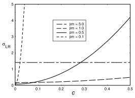
Figure 1: The friction coefficient $\sigma$ as calculated from the linear response formula (4).

The haphazard appearance of the four curves, which have essentially the same shape when viewed on appropriate scales, is explained by a competition between the two terms in (4). Since $\Gamma_{k}$ is proportional to $c$, weak coupling favours the first term, which is a decreasing function of temperature, while strong coupling favours the second term, which increases with temperature.

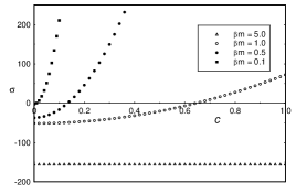
Figure 2: The friction coefficient $\sigma$ as calculated numerically from (21) and (22).

Figure 2 shows $\sigma$ as calculated numerically from equations (21) and (22). Not only does the magnitude differ by factors of several hundred, but $\sigma$ turns out to be negative at weak coupling. (Strictly, it is only at weak coupling that the assumption $\Gamma_{k}\ll\omega_{k}$ holds.) Of course, a negative friction coefficient does not make good physical sense: it clearly reflects the breakdown of the time-derivative expansion noted above.

We estimate the accuracy of the numerical integrals used to obtain $K(k,k^{\prime})$ and to evaluate (7) as about 1%, and have verified the sum rules (23) at this level. The solution of (22) for $\delta n_{k}$ is such that the left and right-hand sides of this equation differ by no more than one part in $10^{7}$ (i.e. the solution is valid to full single-precision accuracy) and we have verified that the whole procedure converges to the results shown as the momentum cutoff used in (7) and (22) is increased.

These results strongly indicate that linear response theory gives the wrong answer to this problem, and the reason may be this. The formula (4) arises from the second term in (3) where, for the mode of momentum $k$, the time integral amounts to an average over a time interval of order $\Gamma_{k}^{-1}$. During this time interval, the actual state of the system changes by an amount of order $\Gamma_{k}^{-1}\dot{\phi}$, so the putative equilibrium state represented by $\langle\ldots\rangle^{\mathrm{eq}}$ is uncertain by an amount of this order. Thus, the first term of (3) is ill-defined by an amount proportional to $\dot{\phi}$ that could well be comparable with, or greater than, the quantity we extract from the second.

Two final remarks are in order. First, the field theory in an expanding universe is equivalent, in conformal time, to a Minkowski-space theory with a mass $m_{\Phi}$ that depends on $a(t)$. Applied to this theory, the time-derivative expansion generates additional terms, proportional to $\dot{a}/a$, which may be important, but do not affect our conclusions about the term proportional to $\dot{\phi}$. Second, the results presented here may be specific to the $\lambda\Phi^{4}$ model. The dynamics of fermions to which $\Phi$ might couple can be represented Lawrie and McKernan (2000) by evolution equations similar to (11) and (12), but $K(k,k^{\prime})$ and $\Gamma_{k}$ are different, and the solution may be very sensitive to this difference.

It is a pleasure to acknowledge discussions with Arjun Berera and Rudnei Ramos, which prompted the study reported here, and to thank Jim Morgan for valuable comments on an earlier version of this paper.

References

- Berera (1995) A. Berera, Phys. Rev. Lett 75, 3218 (1995).
- Berera (2000) A. Berera, Nucl. Phys. B585, 666 (2000).
- Morikawa and Sasaki (1985) M. Morikawa and M. Sasaki, Phys. Lett. B 165, 59 (1985).
- Morikawa and Sasaki (1984) M. Morikawa and M. Sasaki, Prog. Theor. Phys. 72, 782 (1984).
- Hosoya and Sakagami (1984) A. Hosoya and M. Sakagami, Phys. Rev. D 29, 2228 (1984).
- Gleiser and Ramos (1994) M. Gleiser and R. O. Ramos, Phys. Rev. D 50, 2441 (1994).
- Berera and Ramos (2001) A. Berera and R. O. Ramos, Phys. Rev. D 63, 103509 (2001).
- le Bellac (2000) M. le Bellac, Thermal Field Theory (Cambridge University Press, Cambridge, 2000).
- Jeon (1993) S. Jeon, Phys. Rev. D 47, 4586 (1993).
- Jeon (1995) S. Jeon, Phys. Rev. D 52, 3591 (1995).
- Jeon and Yaffe (1996) S. Jeon and L. G. Yaffe, Phys. Rev. D 53, 5799 (1996).
- Aarts and Berges (2001) G. Aarts and J. Berges, Phys. Rev. D 64, 105010 (2001).
- Lawrie (1989) I. D. Lawrie, Phys. Rev. D 40, 3330 (1989).
- Lawrie and McKernan (2000) I. D. Lawrie and D. B. McKernan, Phys. Rev, D 62, 105032 (2000).