MPI-PhT-2002-08
UTHEP-02-0401
Mar., 2002

Quantum Corrections to Newton’s Law^†

B.F.L. Ward^a,b
aWerner-Heisenberg-Institut, Max-Planck-Institut fuer Physik, Muenchen, Germany,
^bDepartment of Physics and Astronomy,
The University of Tennessee, Knoxville, Tennessee 37996-1200, USA.

Abstract

We present a new approach to quantum gravity starting from Feynman’s formulation for the simplest example, that of a scalar field as the representative matter. We show that we extend his treatment to a calculable framework using resummation techniques already well-tested in other problems. Phenomenological consequences for Newton’s law are described.

• Work partly supported by the US Department of Energy Contract DE-FG05-91ER40627 and by NATO Grant PST.CLG.977751.

The law of Newton is the most basic one in physics – it is already taught to beginning students at the most elementary level. Albert Einstein showed that it could be incorporated into his general theory of relativity as a simple special case of the solutions of the respective classical field equations. With the advent of the quantum mechanics of formulations of Heisenberg and Schroedinger, one would have thought that Newton’s law would be the first classical law to be understood completely from a quantum aspect. This, however, has not happened. Indeed, even today, we do not have a quantum treatment of Newton’s law that is known to be correct phenomenologically. In this paper, we propose a possible solution to this problem.

We start from the formulation of Einstein’s theory given by Feynman in Ref. [1, 2]. The respective action density is ( in this paper, like Feynman, we ignore matter spin as an inessential complication [3] )

$$\begin{split}{\cal L}(x)&=-\frac{1}{2\kappa^{2}}R\sqrt{-g}+\frac{1}{2}\left(g^{\mu\nu}\partial_{\mu}\varphi\partial_{\nu}\varphi-m_{o}^{2}\varphi^{2}\right)\sqrt{-g}\\ &=\quad\frac{1}{2}\left\{h^{\mu\nu,\lambda}\bar{h}_{\mu\nu,\lambda}-2\eta^{\mu\mu^{\prime}}\eta^{\lambda\lambda^{\prime}}\bar{h}_{\mu_{\lambda},\lambda^{\prime}}\eta^{\sigma\sigma^{\prime}}\bar{h}_{\mu^{\prime}\sigma,\sigma^{\prime}}\right\}\\ &\qquad+\frac{1}{2}\left\{\varphi_{,\mu}\varphi^{,\mu}-m_{o}^{2}\varphi^{2}\right\}-\kappa{h}^{\mu\nu}\left[\overline{\varphi_{,\mu}\varphi_{,\nu}}+\frac{1}{2}m_{o}^{2}\varphi^{2}\eta_{\mu\nu}\right]\\ &\quad-\kappa^{2}\left[\frac{1}{2}h_{\lambda\rho}\bar{h}^{\rho\lambda}\left(\varphi_{,\mu}\varphi^{,\mu}-m_{o}^{2}\varphi^{2}\right)-2\eta_{\rho\rho^{\prime}}h^{\mu\rho}\bar{h}^{\rho^{\prime}\nu}\varphi_{,\mu}\varphi_{,\nu}\right]+\cdots\\ \end{split}$$ (1)

Here, $\varphi(x)$ is our representative scalar field for matter, $\varphi(x)_{,\mu}\equiv\partial_{\mu}\varphi(x)$, and $g_{\mu\nu}(x)=\eta_{\mu\nu}+2\kappa h_{\mu\nu}(x)$ is the metric of space-time where we follow Feynman and expand about Minkowski space so that $\eta_{\mu\nu}=diag\{1,-1,-1,-1\}$. $R$ is the curvature scalar. Following Feynman, we have introduced the notation $\bar{y}_{\mu\nu}\equiv\frac{1}{2}\left(y_{\mu\nu}+y_{\nu\mu}-\eta_{\mu\nu}{y_{\rho}}^{\rho}\right)$ for any tensor $y_{\mu\nu}$. Thus, $m_{o}$ is the bare mass of our matter and we set the small tentatively observed [4] value of the cosmological constant to zero so that our quantum graviton has zero rest mass. Here, our normalizations are such that $\kappa=\sqrt{8\pi G_{N}}$ where $G_{N}$ is Newton’s constant. The Feynman rules for (1) have been essentially worked out by Feynman [1, 2], including the rule for the famous Feynman-Faddeev-Popov [1, 5] ghost contribution that must be added to it to achieve a unitary theory with the fixing of the gauge ( we use the gauge of Feynman in Ref. [1], $\partial^{\mu}\bar{h}_{\nu\mu}=0$ ), so we do not repeat this material here. We go instead directly to the treatment of the apparently uncontrolled UV divergences associated with (1).

To illustrate our approach, let us study the possible one-loop corrections to Newton’s law that would follow from the matter in (1) assuming that our representative matter is really part of a multiplet of fields at a very high scale ( $M_{GUT}=10^{16}$GeV ) compared to the known SM particles so that it is sufficient to calculate the effects of the diagrams in Fig. 11 on the graviton propagator to see the first quantum loop effect.

Figure 1: The scalar one-loop contribution to the graviton propagator. $q$ is the 4-momentum of the graviton.

To this end, we stress the following. The naive power counting of the graphs give their degree of divergence as +4 and we expect that even with the gauge invariance there will still remain at least a 0 degree of divergence and that, in higher orders, this remaining divergence degree gets larger and larger. Indeed, for example, for Fig. 1a, we get the result

$$i\Sigma(q)^{1a}_{\bar{\mu}\bar{\nu};\mu\nu}=\kappa^{2}\frac{\int d^{4}k}{2(2\pi)^{4}}\frac{\left(k^{\prime}_{\bar{\mu}}k_{\bar{\nu}}+k^{\prime}_{\bar{\nu}}k_{\bar{\mu}}\right)\left(k^{\prime}_{\mu}k_{\nu}+k^{\prime}_{\nu}k_{\mu}\right)}{\left({k^{\prime}}^{2}-m^{2}+i\epsilon\right)\left(k^{2}-m^{2}+i\epsilon\right)}$$ (2)

, where we set $k^{\prime}=k+q$ and we take for definiteness only fully transverse, traceless polarization states of the graviton to be act on $\Sigma$ so that we have dropped the traces from its vertices. Clearly, (2) has degree of divergence +4. Explicit use of the Feynman rules for (1) shows indeed that this superficial divergence degree gets larger and larger as we go to higher and higher loop contributions.

However, there is a physical effect which must be taken into account in a situation such as that in Fig. 1. Specifically, the gravitational force is attractive and proportional to $(mass)^{2}$, so that as one goes with the integration four-momentum $k$ into the deep Euclidean (large negative $(mass)^{2}$) $k^{2}$ regime ( assume we have Wick rotated henceforth ), the ‘attractive’ force from gravity between the particle at a point $x$ and one at point $x^{\prime}$ becomes ’repulsive’ and should cause the respective propagator between the two points to be damped severely in the exact solutions of the theory. This suggests that we should resum the soft graviton corrections to the propagators in Fig. 1 to get an improved and physically more meaningful result.

We point out that the procedure of resumming the propagators in a theory to get a more meaningful and physically more accurate result is well founded in recent years. The precision Z physics tests at SLC/LEP1 and the precision WW pair production tests at LEP2 [6] of the SM are all based on comparisons between experiment and theory in which Dyson resummed Z and W boson propagators are essential. For example, in Refs. [7], one can see that SM one-loop corrections involving the exchange of Z’s and W’s in the respective loops are calculated sytematically using Dyson resummed propagators and these one-loop corrections have been found to be in agreement with experiment [6]. Here, we seek to follow the analogous path, where instead of making a Dyson resummation of our propagators we will make a soft graviton resummation of these propagators.

We use the formulas of Yennie, Frautschi and Suura (YFS) [8], which we have used with success in many higher order resummation applications for precision Standard Model [9] EW tests at LEP1/SLC and at LEP2, to resum the the propagators in Fig. 1 and use their resummed versions in the loop expansion just as the Dyson resummed W and Z propagators are used in the loop calculations in Refs. [7]. To this end, we need to determine the analogue for gravitons of the YFS virtual infrared (IR) function $\alpha B^{\prime\prime}\equiv\alpha B^{\prime\prime}_{\gamma}$ in eq.(5.16) of Ref. [8] which gives the respective YFS resummation of the soft photon corrections for the electron proper self-energy $\Sigma_{F}$ in QED:

$$\Sigma_{F}(p)=e^{\alpha B^{\prime\prime}_{\gamma}}\left[{\Sigma^{\prime}}_{F}(p)-S^{-1}_{F}(p)\right]+S^{-1}_{F}(p),$$ (3)

as this latter equation implies the YFS resummed electron propagator result

$$iS^{\prime}_{F}(p)=\frac{ie^{-\alpha B^{\prime\prime}_{\gamma}}}{S^{-1}_{F}(p)-{\Sigma^{\prime}}_{F}(p)}.$$ (4)

Here, ${\Sigma^{\prime}}_{F}(p)$ is proper self-energy hard photon residual corresponding directly to the sum over the hard photon residuals on the RHS of eq.(2.3) of Ref. [8]:

$${\Sigma^{\prime}}_{F}(p)=\sum_{n=1}^{\infty}{\Sigma^{\prime}}_{Fn},$$ (5)

where ${\Sigma^{\prime}}_{Fn}$ is the n-loop YFS IR subtracted residual contribution to $\Sigma_{F}$ which is free of virtual IR singularities and which is defined in Ref. [8], i.e., we follow directly the development in Ref. [8] as it is applied there to the proper one-particle irreducible two-point function for the electron, the inverse propagator function. We stress that (4) is an exact re-arrangement of the respective Feynman-Schwinger-Tomonaga series valid at all energies. We also stress that, as the probability to radiate soft quanta in high energy annihilation processes for a particle of mass m and charge e is proportional to [8] $2\frac{\alpha}{\pi}\left(\ln s/m^{2}-1\right)$, where $s=4E^{2}$ when $E$ is the cms energy, the effects of such resummation become more and more important at higher and higher energies. From eq.(5.13) of Ref. [8], we have the representation

$$\alpha B^{\prime\prime}_{\gamma}=\int d^{4}\ell\frac{S^{\prime\prime}(k,k,\ell)}{\ell^{2}-\lambda^{2}+i\epsilon}$$ (6)

where $\lambda$ is the usual infrared regulator and the YFS virtual IR emission function is given by

$$S^{\prime\prime}(k,k,\ell)=\frac{-i8\alpha}{(2\pi)^{3}}\frac{kk^{\prime}}{(\ell^{2}-2\ell k+\Delta+i\epsilon)(\ell^{2}-2\ell k^{\prime}+\Delta^{\prime}+i\epsilon)}{\Big{|}}_{k=k^{\prime}}$$ (7)

where we define $\Delta=k^{2}-m^{2}$, $\Delta^{\prime}={k^{\prime}}^{2}-m^{2}$. We see that we may also write (6) as

$$\alpha B^{\prime\prime}_{\gamma}=\int\frac{d^{4}\ell}{(2\pi)^{4}}\frac{-i\eta^{\mu\nu}}{(\ell^{2}-\lambda^{2}+i\epsilon)}\frac{-ie(2ik_{\mu})}{(\ell^{2}-2\ell k+\Delta+i\epsilon)}\frac{-ie(2ik^{\prime}_{\nu})}{(\ell^{2}-2\ell k^{\prime}+\Delta^{\prime}+i\epsilon)}{\Big{|}}_{k=k^{\prime}}.$$ (8)

Using the results in Appendix A of Ref. [8], this allows us to write down the corresponding result for the soft graviton virtual IR emission process, where, following Weinberg in Ref. [13] and using the Feynman rules for (1), we identify the conserved charges in the graviton case as $e\rightarrow\kappa k_{\rho}$ for soft emission from k so that for the analogue of the virtual YFS function $\alpha B^{\prime\prime}_{\gamma}$ we get here the graviton virtual IR function $-B^{\prime\prime}_{g}(k)$ given by replacing the photon propagator in (8) by the graviton propagator,

$$\frac{i\frac{1}{2}(\eta^{\mu\nu}\eta^{\bar{\mu}\bar{\nu}}+\eta^{\mu\bar{\nu}}\eta^{\bar{\mu}\nu}-\eta^{\mu\bar{\mu}}\eta^{\nu\bar{\nu}})}{\ell^{2}-\lambda^{2}+i\epsilon}$$

, and by replacing the QED charges by the corresponding gravity charges $\kappa k_{\bar{\mu}},~{}\kappa k^{\prime}_{\bar{\nu}}$. In this way we get the result

$$B^{\prime\prime}_{g}(k)=-2i\kappa^{2}k^{4}\frac{\int d^{4}\ell}{16\pi^{4}}\frac{1}{\ell^{2}-\lambda^{2}+i\epsilon}\frac{1}{(\ell^{2}+2\ell k+\Delta+i\epsilon)^{2}}$$ (9)

and the corresponding scalar version of (4) as

$$i\Delta^{\prime}_{F}(k)|_{YFS-resummed}=\frac{ie^{B^{\prime\prime}_{g}(k)}}{(k^{2}-m^{2}-\Sigma^{\prime}_{s}+i\epsilon)}$$ (10)

where the YFS soft graviton infrared subtracted residual $\Sigma^{\prime}_{s}$ is in quantum gravity the scalar analogue of the QED electron proper self-energy soft photon IR subtracted residual $\Sigma^{\prime}_{F}$. As $\Sigma^{\prime}_{s}$ starts in ${\cal O}(\kappa^{2})$, we may drop it in using the result (10) in calculating the one-loop effects in Fig. 1. We also stress that, unlike its QED counterpart, this quantum gravity soft graviton YFS IR subtracted residual is not completely free of virtual IR singularities: the genuine non-Abelian soft graviton IR singularities are still present in it. These can be computed and handled order by order in $\kappa$ in complete analogy with what is done in QCD [14] perturbation theory. For the deep Euclidean regime relevant to (2), we get

$$B^{\prime\prime}_{g}(k)=\frac{\kappa^{2}|k^{2}|}{8\pi^{2}}\ln\left(\frac{m^{2}}{m^{2}+|k^{2}|}\right)$$ (11)

so that, as we expected, the soft graviton resummation following the rigorous YFS prescription causes the propagators in (2) to be damped faster than any power of $|k^{2}|$! ( For the massless case where the renormalized mass $m$ vanishes, the result (11) is best computed using the customary $-\mu^{2}$ normalization point for massless particles. In this way, we get $B^{\prime\prime}_{g}(k)=\frac{\kappa^{2}|k^{2}|}{8\pi^{2}}\ln\left(\frac{\mu^{2}}{|k^{2}|}\right)$ in the deep Euclidean regime for the massless case, where $-\mu^{2}$ can be identified as the respective (re)normalization point. This again falls faster than any power of $|k^{2}|$!) When we introduce the result (11) into (2), we get ( here, $k\rightarrow(ik^{0},\vec{k})$ by Wick rotation )

$$i\Sigma(q)^{1a}_{\bar{\mu}\bar{\nu};\mu\nu}=i\kappa^{2}\frac{\int d^{4}k}{2(2\pi)^{4}}\frac{\left(k^{\prime}_{\bar{\mu}}k_{\bar{\nu}}+k^{\prime}_{\bar{\nu}}k_{\bar{\mu}}\right)e^{\frac{\kappa^{2}|{k^{\prime}}^{2}|}{8\pi^{2}}\ln\left(\frac{m^{2}}{m^{2}+|{k^{\prime}}^{2}|}\right)}\left(k^{\prime}_{\mu}k_{\nu}+k^{\prime}_{\nu}k_{\mu}\right)e^{\frac{\kappa^{2}|k^{2}|}{8\pi^{2}}\ln\left(\frac{m^{2}}{m^{2}+|k^{2}|}\right)}}{\left({k^{\prime}}^{2}-m^{2}+i\epsilon\right)\left(k^{2}-m^{2}+i\epsilon\right)}.$$ (12)

Evidently, this integral converges; so does that for Fig.1b when we use the improved resummed propagators. This means that we have a rigorous quantum loop correction to Newton’s law from Fig.1 which is finite and well defined.

More precisely, using standard resummation algebra already well-tested in precision EW physics as cited above, we replace the naive free propagator

$$i\Delta_{F}(k)=\frac{i}{(k^{2}-m^{2}+i\epsilon)}$$

with the resummed “improved Born” propagator

$$\begin{split}i{\Delta}^{(0)}_{F}(k)|_{YFS-resummed}&=\frac{ie^{B^{\prime\prime}_{g}(k)}}{(k^{2}-m^{2}+i\epsilon)}\\ &=i\Delta^{\prime}_{F}(k)|_{YFS-resummed,\Sigma^{\prime}_{s}=0}\end{split}$$ (13)

everywhere in the loop expansions of our theory, with due attention to avoid double counting, as usual. In this way, one sees that ${\Delta}^{(0)}_{F}(k)|_{YFS-resummed}$ is also used in computing the residual $\Sigma^{\prime}_{s}(k)$ as well, so that $\Sigma^{\prime}_{s}(k)$ is now also finite and indeed makes at most a small genuine two-loop, suppressed by ${\cal O}(\kappa^{2})$, correction to the improved calculation of the one-loop corrections in Fig. 1 that we get by using our improved propagator $i{\Delta}^{(0)}_{F}(k)|_{YFS-resummed}$ therein. This rigorously justifies neglecting $\Sigma^{\prime}_{s}(k)$ when we work to leading order $\kappa^{2}$.

Let us examine the entire theory from (1) to all orders in $\kappa$: we write it as

$${\cal L}(x)={\cal L}_{0}(x)+\sum_{n=1}^{\infty}\kappa^{n}{\cal L}_{I}^{(n)}(x)$$ (14)

in an obvious notation in which the first term is the free Lagrangian, including the free part of the gauge-fixing and ghost Lagrangians and the interactions, including the ghost interactions, are the terms of ${\cal O}(\kappa^{n}),n\geq 1$.

Each ${\cal L}_{I}^{(n)}$ is itself a finite sum of terms:

$${\cal L}_{I}^{(n)}(x)=\sum_{\ell=1}^{m_{n}}{\cal L}_{I,\ell}^{(n)}(x).$$ (15)

${\cal L}_{I,\ell}^{(n)}$ has dimension $d_{n,\ell}$. Let $d^{M}_{n}=\max_{\ell}\{d_{n,\ell}\}$. As we have at least three fields at each vertex, the maximum power of momentum at any vertex in ${\cal L}_{I}^{(n)}$ is $\bar{d}^{M}_{n}=\min\{d^{M}_{n}-3,2\}$ and is finite ( here, we use the fact that the Riemann tensor is only second order in derivatives ). We will use this fact shortly.

First we stress that, in any gauge, if $P_{\alpha_{1}\cdots;\alpha^{\prime}_{1}\cdots}$ is the respective propagator polarization sum for a spinning particle, then the spin independence of the soft graviton YFS resummation exponential factor in (13) yields the respective YFS resummed improved Born propagator as

$$i{\cal D}^{(0)}_{F\alpha_{1}\cdots;\alpha^{\prime}_{1}\cdots}(k)|_{YFS-resummed}=\frac{iP_{\alpha_{1}\cdots;\alpha^{\prime}_{1}\cdots}e^{B^{\prime\prime}_{g}(k)}}{(k^{2}-m^{2}+i\epsilon)},$$ (16)

so that it is also exponentially damped at high energy in the deep Euclidean regime (DER). We will use this shortly as well.

Now consider any one particle irreducible vertex $\Gamma_{N}$ with $[N]\equiv n_{1}+n_{2}$ amputated external legs, where we use the notation $N=(n_{1},n_{2})$, when $n_{1}(n_{2})$ is the respective number of graviton(scalar) external lines. We always assume we have Wick rotated. At its zero-loop order, there are only tree contributions which are manifestly UV finite. Consider the first loop (${\cal O}(\kappa^{2})$) corrections to $\Gamma_{N}$. There must be at least one improved exponentially damped propagator in the respective loop contribution and at most two vertices so that the maximum power of momentum in the numerator of the loop due to the vertices is $\max\{2\bar{d}^{M}_{1},\bar{d}^{M}_{2}\}$ and is finite. The exponentially damped propagator then renders the loop integrals finite and as there are only a finite number of them, the entire one-loop (${\cal O}(\kappa^{2})$) contribution is finite.

As a corollary, if $\Gamma_{N}$ vanishes in tree approximation, we can conclude that its first non-trivial contributions at one-loop are all finite, as in each such loop the exponentially damped propagator which must be present is sufficient to damp the respective finite order polynomial in loop momentum that occurs from its vertices by our arguments above into a convergent integral.

As an induction hypothesis suppose all contributions to all $\{\Gamma_{N}\}$ for m-loop corrections (${\cal O}(\kappa^{2m})),m<n,$ are finite. At the n-loop (${\cal O}(\kappa^{2n})$) level, when the exponentially damped improved Born propagators are taken into account, we argue that respective n-loop integrals are finite as follows. First, by momentum conservation, if $\{\ell_{1},\cdots,\ell_{n}\}$ are the respective Euclidean loop momenta, we may without loss of content assume that $\ell_{n}$ is precisely the momentum of one of the exponentially damped improved Born propagators. The $n-1$ loop integrations over the remaining loop variables $\{\ell_{1},\cdots,\ell_{n-1}\}$ for fixed $\ell_{n}$ then produces the contribution of a subgraph which if it is 1PI is a part of $\Gamma_{N+2}$ and which if it is not 1PI is a product of the contributions to the respective $\{\Gamma_{J}\}$ and the respective improved YFS resummed Born propagator functions. This is then finite by the induction hypothesis. Here, $N+2=(n_{1}+2,n_{2})\left((n_{1},n_{2}+2)\right)$ according as the propagator with momentum $\ell_{n}$ which we fix as multiplying the remaining subgraph is a graviton(scalar) propagator, respectively. The application of standard arguments [15] from Lebesgue integration theory ( specifically, for any two measurable functions $f,g$, $f\leq g$ almost everywhere implies that $\int f\leq\int g$ ) in conjunction with Weinberg’s theorem [16] guarantees that this finite result behaves at most as a finite power of $|\ell_{n}|$ modulo Weinberg’s logarithms for $|\ell_{n}|\rightarrow\infty$. It follows that the remaining integration over $\ell_{n}$ is damped into convergence by the already identified exponentially damped propagator with momentum $\ell_{n}$. Thus, each $n$-loop contribution to $\Gamma_{N}$ is finite, from which it follows that $\Gamma_{N}$ is finite at $n$-loop level. Pictorially, we illsutrate the type of situations we have in Fig. 2.

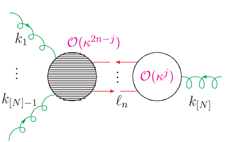
Figure 2: The typical contribution we encounter in $\Gamma_{N}$ at the n-loop level; $\ell_{n}$ is the n-th loop momentum and is precisely the momentum of the indicated YFS-resummed improved Born propagator.

We conclude by induction that all $\{\Gamma_{N}\}$ in our theory are finite to all orders in the loop expansion. Of course, the sum of the respective series in $\kappa$ may very well not actually converge but this issue is beyond the scope of our work.

The key in the argument is the ability to isolate, for example in the scalar propagator, the YFS soft graviton infrared subtracted residual $\Sigma_{s}^{\prime}$ order by order in our new improved loop expansion. We stress that since we have an identity in (10) we have not altered the Feynman-Schwinger-Tomonaga series; we have just re-arranged it so that we treat $\Sigma_{s}^{\prime}$ perturbatively relative to our improved Born YFS-resummed propagator in complete analogy with the treatment of the usual $\Sigma_{s}$ perturbatively relative to the naive Feynman propagator $i\Delta_{F}$. To see that this makes sense, let us write down $\Sigma_{s}^{\prime}(k)$ explicitly in one loop order.

We have from (10) the one-loop result

$$\Sigma_{s}^{{}^{\prime}(1)}(k)=\Sigma_{s}^{(1)}(k)-B^{\prime\prime}_{g}(k)\Delta_{F}^{-1}(k)$$ (17)

where $A^{(n)}$ is the n-loop contribution to $A$. Using the standard methods, we see that this allows us to get the following representation of $\Sigma_{s}^{{}^{\prime}(1)}(k)$ in our YFS-resummed improved perturbation theory:

$$\begin{split}\Sigma_{s}^{{}^{\prime}(1)}(k)&=-\kappa^{2}\frac{\int d^{4}\ell}{(2\pi)^{4}}\Bigg{\{}\Big{[}(2k^{\mu}k^{\nu}){\cal P}_{\mu\nu;\mu^{\prime}\nu^{\prime}}(\ell)(2k^{\mu^{\prime}}k^{\nu^{\prime}})\frac{\ell^{2}+2\ell k+2(k^{2}-m^{2})}{\ell^{2}+2\ell k+k^{2}-m^{2}+i\epsilon}\\ &+\quad\Delta V^{\mu\nu}(k,\ell){\cal P}_{\mu\nu;\mu^{\prime}\nu^{\prime}}(\ell)(2k^{\mu^{\prime}}k^{\nu^{\prime}})+(2k^{\mu}k^{\nu}){\cal P}_{\mu\nu;\mu^{\prime}\nu^{\prime}}(\ell)\Delta V^{\mu^{\prime}\nu^{\prime}}(k,\ell)\\ &+\quad\Delta V^{\mu\nu}(k,\ell){\cal P}_{\mu\nu;\mu^{\prime}\nu^{\prime}}(\ell)\Delta V^{\mu^{\prime}\nu^{\prime}}(k,\ell)\Big{]}\frac{e^{\frac{\kappa^{2}|(k+\ell)^{2}|}{8\pi^{2}}\ln\left(\frac{m^{2}}{m^{2}+|(k+\ell)^{2}|}\right)}}{(k+\ell)^{2}-m^{2}+i\epsilon}\frac{e^{\frac{\kappa^{2}|\ell^{2}|}{8\pi^{2}}\ln\left(\frac{\mu^{2}}{|\ell^{2}|}\right)}}{\ell^{2}+i\epsilon}\\ &+\quad\Big{[}\frac{1}{2}(k^{2}-m^{2})\left({{\cal P}_{\lambda\rho;}}^{\rho\lambda}(\ell)+{{\cal P}_{\lambda\rho;}}^{\lambda\rho}(\ell)-{{{{\cal P}_{\lambda}}^{\lambda}}_{;\lambda^{\prime}}}^{\lambda^{\prime}}(\ell)\right)\\ &-\quad(2k^{\mu}k^{\nu})\left({{{\cal P}_{\mu\rho;}}^{\rho}}_{\nu}(\ell)+{{\cal P}_{\mu\rho;\nu}}^{\rho}(\ell)-{{\cal P}_{\mu\nu;\rho}}^{\rho}(\ell)\right)\Big{]}\frac{e^{\frac{\kappa^{2}|\ell^{2}|}{8\pi^{2}}\ln\left(\frac{\mu^{2}}{|\ell^{2}|}\right)}}{\ell^{2}+i\epsilon}\Bigg{\}},\end{split}$$ (18)

where we have defined $\Delta V^{\mu\nu}(k,\ell)=k^{\mu}\ell^{\nu}+k^{\nu}\ell^{\mu}-(k^{2}-m^{2}+k\ell)\eta^{\mu\nu}$. We see explicitly that the exponentially damped propagators render $\Sigma_{s}^{{}^{\prime}(1)}(k)$ ultra-violet (UV) finite. It is clear from (18) that $\Sigma_{s}^{\prime}$ is indeed a small perturbation on our results in this paper and we can neglect it in what follows. It will be presented in detail elsewhere.

Continuing to work in the transverse, traceless space for $\Sigma$, we get, to leading order, that the graviton propagator denominator becomes

$$q^{2}+\frac{1}{2}q^{4}\Sigma^{T^{\prime\prime}}(0)+i\epsilon$$ (19)

where the self-energy function $\Sigma^{T}(q^{2})$ follows from Fig. 1 by the standard methods ( the new type of integral we do by steepest descent considerations for this paper ) and for its second derivative at $q^{2}=0$ we have the result

$$\begin{split}\Sigma^{T^{\prime\prime}}(0)&=-\frac{\kappa^{4}m^{2}f_{sd}}{8\pi^{3}\sqrt{\pi}}\frac{240}{786432}\ln^{3}x_{0}\left(1-\frac{135}{4096c_{sd}}\ln x_{0}\right)\\ &\simeq-\frac{7.44m^{2}f_{sd}}{\pi^{2}M_{Pl}^{4}},\end{split}$$ (20)

where $M_{Pl}=1.22\times 10^{19}$GeV is the Planck mass , $x_{0}=\frac{\pi}{2}\frac{M^{2}_{Pl}}{m^{2}c_{sd}}$ and we work in the leading log approximation for the big log $L=\ln x_{0}$. The steepest descent factors $c_{sd},f_{sd}$ turn out to be $c_{sd}\simeq 12.9,~{}f_{sd}\simeq 5.79\times 10^{2}$.

To see the effect on Newton’s potential, we Fourier transform the inverse of (19) and find the potential

$$\Phi_{Newton}(r)=-\frac{G_{N}M_{1}M_{2}}{r}(1-e^{-ra})$$ (21)

where $a=1/\sqrt{-\frac{1}{2}\Sigma^{T^{\prime\prime}}(0)}\simeq 82.6M_{Pl}$ in an obvious notation. With the current experimental accuracy [17] on $G_{N}$ of $\pm 0.15\%$, we see that, to be sensitive to this quantum effect, we must reach distances $\sim 6.45\times 10^{-21}GeV^{-1}\simeq 0.13\times 10^{-33}cm$. Presumably, in the early universe studies [18], this is available . This opens the distinct possibility that physics below the Planck scale is accessible to point particle quantum field theoretic methods.

We believe then that we have found a systematic approach to computing quantum gravity as formulated by Feynman in Ref. [1, 2]. The law of Newton may now be studied on equal footing with the other known forces in the Standard Model [9] of $SU_{c}(3)\times SU_{2L}\times U_{1}$ interactions.

Notes Added

1. The limit of quantum gravity studied here is that of the deep Euclidean regime, i.e., the short-distance limit of the theory. This should be contrasted with the long-distance limit studied by effective Lagrangian methods such as those used in Ref. [25].

2. That we get a cut-off at $\sim M_{Pl}$ in our theory means that, if the improved propagators we find are introduced into the renormalizable SM Feynman rules, the net effect will be to cut-off the respective Feynman integrals at $\sim M_{Pl}$ and ,hence, by the standard results of renormalizable quantum field theory, there will no effect on any of the phenomenological predictions of the SM at scales well below $M_{Pl}$.

3. For nonrenormalizable theories, our methods appear to offer a ‘new lease’ on life for many of them. We caution that, while our improved propagators render many of them finite, they may have other problems.

References

- [1] R. P. Feynman, Acta Phys. Pol. 24 (1963) 697.
- [2] R. P. Feynman, Feynman Lectures on Gravitation, eds. F.B. Moringo and W.G. Wagner (Caltech, Pasadena, 1971).
- [3] M.L. Goldberger, private communication, 1972.
- [4] S. Perlmutter et al., Astrophys. J. 517 (1999) 565; and, references therein.
- [5] L. D. Faddeev and V.N. Popov, ITF-67-036, NAL-THY-57 (translated from Russian by D. Gordon and B.W. Lee); Phys. Lett. B25 (1967) 29.
- [6] D. Abbaneo et al., hep-ex/0112021.
- [7] See, for example, M. Grunewald et al., CERN-2000-09-A, in Proc. 2000 LEP2 Workshop, eds. S. Jadach et al., (CERN, Geneva, 2000) p. 1; M. Kobel et al., op. cit., p. 269, CERN-2000-09-D; D. Bardin et al. in Proc. 1994-1995 LEP1 Workshop, eds. D. Bardin, W. Hollik and G. Passarino, ( CERN, Geneva, 1995 ) p.7, and references therein.
-
[8]
D. R. Yennie, S. C. Frautschi, and H. Suura, Ann. Phys. 13 (1961) 379;
see also K. T. Mahanthappa, Phys. Rev. 126 (1962) 329, for a related analysis. - [9] S.L. Glashow, Nucl. Phys. 22 (1961) 579; S. Weinberg, Phys. Rev. Lett. 19 (1967) 1264; A. Salam, in Elementary Particle Theory, ed. N. Svartholm (Almqvist and Wiksells, Stockholm, 1968), p. 367; G. ’t Hooft and M. Veltman, Nucl. Phys. B44,189 (1972) and B50, 318 (1972); G. ’t Hooft, ibid. B35, 167 (1971); M. Veltman, ibid. B7, 637 (1968).
- [10] S. Jadach et al., Comput. Phys. Commun. 102 (1997) 229.
- [11] S. Jadach, M. Skrzypek and B.F.L. Ward, Phys.Rev. D55 (1997) 1206.
- [12] G. Montagna, M. Moretti, O. Nicrosini, A. Pallavicini, and F. Piccinini, Phys. Lett. B459 (1999) 649.
- [13] S. Weinberg, The Quantum Theory of Fields, vols. 1-3, ( Cambridge University Press, Cambridge, 1995 ).
- [14] R. D. Field, Applications of Perturbative QCD, ( Addison-Wesley Publ. Co., Redwood City, 1989 ).
- [15] H.L. Royden, Real Analysis, (MacMillan Co., New York, 1968 ).
- [16] S. Weinberg, Phys. Rev. 118 (1960) 838; K. Hepp, Commun. Math. Phys. 2 (1966) 301.
- [17] D. E. Groom et al., Eur. Phys. J. C15 (2000) 1.
- [18] E. W. Kolb, in Proc. ICHEP98, v.1., eds. A. Astbury, D. Axen and J. Robinson ( World Scientific, Singapore, 1999) p. 347.
- [19] See, for example, J. Schwarz, in Proc. Berkeley Chew Jubilee, 1984, eds. C. DeTar et al. ( World Scientific, Singapore, 1985 ) p. 106, and references therein.
- [20] See, for example, R. E. Taylor, Phil. Trans. Roy. Soc. Lond. A359 (2001) 225, and references therein.
- [21] See, for example, J. Bjorken (SLAC), in Proc. 3rd International Symposium on the History of Particle Physics: The Rise of the Standard Model, Stanford, CA, 1992, eds. L. Hoddeson et al. (Cambridge Univ. Press, Cambridge, 1997) p. 589, and references therein.
- [22] D. J. Gross and F. Wilczek, Phys. Rev. Lett. 30 (1973) 1343; H. David Politzer, ibid.30 (1973) 1346; see also , for example, F. Wilczek, in Proc. 16th International Symposium on Lepton and Photon Interactions, Ithaca, 1993, eds. P. Drell and D.L. Rubin (AIP, NY, 1994) p. 593, and references therein.
- [23] See, for example, M. Green, J. Schwarz and E. Witten, Superstring Theory, v. 1 and v.2, ( Cambridge Univ. Press, Cambridge, 1987 ) and references therein.
- [24] See, for example, J. Polchinski, String Theory, v. 1 and v. 2, (Cambridge Univ. Press, Cambridge, 1998), and references therein.
- [25] See for example J. Donoghue, Phys. Rev. Lett. 72 (1994) 2996; Phys. Rev. D50 (1994) 3874; preprint gr-qc/9512024; J. Donoghue et al., Phys. Lett. B529 (2002) 132, and references therein.