DESY 02–040

UAB–FT–523

hep–ph/0204101

April 2002

Exploring CP Violation through Correlations in

$B\to\pi K$, $B_{d}\to\pi^{+}\pi^{-}$, $B_{s}\to K^{+}K^{-}$ Observable Space

Robert Fleischer

Deutsches Elektronen-Synchrotron DESY, Notkestraße 85, D–22607 Hamburg, Germany

Joaquim Matias
IFAE, Universitat Autònoma de Barcelona, E–08193 Barcelona, Spain

Abstract
We investigate allowed regions in observable space of $B\to\pi K$, $B_{d}\to\pi^{+}\pi^{-}$ and $B_{s}\to K^{+}K^{-}$ decays, characterizing these modes in the Standard Model. After a discussion of a new kind of contour plots for the $B\to\pi K$ system, we focus on the mixing-induced and direct CP asymmetries of the decays $B_{d}\to\pi^{+}\pi^{-}$ and $B_{s}\to K^{+}K^{-}$. Using experimental information on the CP-averaged $B_{d}\to\pi^{\mp}K^{\pm}$ and $B_{d}\to\pi^{+}\pi^{-}$ branching ratios, the relevant hadronic penguin parameters can be constrained, implying certain allowed regions in observable space. In the case of $B_{d}\to\pi^{+}\pi^{-}$, an interesting situation arises now in view of the recent $B$-factory measurements of CP violation in this channel, allowing us to obtain new constraints on the CKM angle $\gamma$ as a function of the $B^{0}_{d}$–$\overline{B^{0}_{d}}$ mixing phase $\phi_{d}=2\beta$, which is fixed through ${\cal A}_{\rm CP}^{\rm mix}(B_{d}\to J/\psi K_{\rm S})$ up to a twofold ambiguity. If we assume that ${\cal A}_{\rm CP}^{\rm mix}(B_{d}\to\pi^{+}\pi^{-})$ is positive, as indicated by recent Belle data, and that $\phi_{d}$ is in agreement with the “indirect” fits of the unitarity triangle, also the corresponding values for $\gamma$ around $60^{\circ}$ can be accommodated. On the other hand, for the second solution of $\phi_{d}$, we obtain a gap around $\gamma\sim 60^{\circ}$. The allowed region in the space of ${\cal A}_{\rm CP}^{\rm mix}(B_{s}\to K^{+}K^{-})$ and ${\cal A}_{\rm CP}^{\rm dir}(B_{s}\to K^{+}K^{-})$ is very constrained in the Standard Model, thereby providing a narrow target range for run II of the Tevatron and the experiments of the LHC era.

1 Introduction

One of the most exciting aspects of present particle physics is the exploration of CP violation through $B$-meson decays, allowing us to overconstrain both the sides and the three angles $\alpha$, $\beta$ and $\gamma$ of the usual non-squashed unitarity triangle of the Cabibbo–Kobayashi–Maskawa (CKM) matrix [1]. Besides the “gold-plated” mode $B_{d}\to J/\psi K_{\rm S}$ [2], which has recently led to the observation of CP violation in the $B$ system [3, 4], there are many different avenues we may follow to achieve this goal.

In this paper, we first consider $B\to\pi K$ modes [5]–[14], and then focus on the $B_{d}\to\pi^{+}\pi^{-}$, $B_{s}\to K^{+}K^{-}$ system [15], providing promising strategies to determine $\gamma$. In a previous paper [16], we pointed out that these non-leptonic $B$ decays can be characterized efficiently within the Standard Model through allowed regions in the space of their observables. If future measurements should result in values for these quantities lying significantly outside of these regions, we would have an immediate indication for the presence of new physics. On the other hand, a measurement of observables lying inside these regions would allow us to extract values for the angle $\gamma$, which may then show discrepancies with other determinations, thereby also indicating new physics. Since penguin processes play a key rôle in $B\to\pi K$, $B_{d}\to\pi^{+}\pi^{-}$ and $B_{s}\to K^{+}K^{-}$ decays, these transitions actually represent sensitive probes for physics beyond the Standard Model [17].

Besides an update and extended discussion of the allowed regions in observable space of appropriate combinations of $B\to\pi K$ decays, following [16], the main point of the present paper is a detailed analysis of the $B_{d}\to\pi^{+}\pi^{-}$, $B_{s}\to K^{+}K^{-}$ system in the light of recent experimental data. These neutral $B$-meson decays into final CP eigenstates provide a time-dependent CP asymmetry of the following form:

$$a_{\rm CP}(t)\equiv\frac{\Gamma(B^{0}_{q}(t)\to f)-\Gamma(\overline{B^{0}_{q}}(t)\to f)}{\Gamma(B^{0}_{q}(t)\to f)+\Gamma(\overline{B^{0}_{q}}(t)\to f)}$$ (1)

$$=\left[\frac{{\cal A}_{\rm CP}^{\rm dir}(B_{q}\to f)\,\cos(\Delta M_{q}t)+{\cal A}_{\rm CP}^{\rm mix}(B_{q}\to f)\,\sin(\Delta M_{q}t)}{\cosh(\Delta\Gamma_{q}t/2)-{\cal A}_{\rm\Delta\Gamma}(B_{q}\to f)\,\sinh(\Delta\Gamma_{q}t/2)}\right],$$

where we have separated, as usual, the “direct” from the “mixing-induced” CP-violating contributions. The time-dependent rates refer to initially, i.e. at time $t=0$, present $B^{0}_{q}$- or $\overline{B^{0}_{q}}$-mesons, $\Delta M_{q}>0$ denotes the mass difference of the $B_{q}$ mass eigenstates, and $\Delta\Gamma_{q}$ is their decay width difference, which is negligibly small in the $B_{d}$ system, but may be as large as ${\cal O}(10\%)$ in the $B_{s}$ system [18]. The three observables in (1) are not independent from one another, but satisfy the following relation:

$$\Bigl{[}{\cal A}_{\rm CP}^{\rm dir}(B_{q}\to f)\Bigr{]}^{2}+\Bigl{[}{\cal A}_{\rm CP}^{\rm mix}(B_{q}\to f)\Bigr{]}^{2}+\Bigl{[}{\cal A}_{\rm\Delta\Gamma}(B_{q}\to f)\Bigr{]}^{2}=1.$$ (2)

If we employ the $U$-spin flavour symmetry of strong interactions, relating down and strange quarks to each other, the CP-violating observables provided by $B_{d}\to\pi^{+}\pi^{-}$ and $B_{s}\to K^{+}K^{-}$ allow a determination both of $\gamma$ and of the $B^{0}_{d}$–$\overline{B^{0}_{d}}$ mixing phase $\phi_{d}$, which is given by $2\beta$ in the Standard Model [15]. Moreover, interesting hadronic penguin parameters can be extracted as well, consisting of a CP-conserving strong phase, and a ratio of strong amplitudes, measuring – sloppily speaking – the ratio of penguin- to tree-diagram-like contributions to $B_{d}\to\pi^{+}\pi^{-}$. The use of $U$-spin arguments in this approach can be minimized, if we use $\phi_{d}$ as an input. As is well known, this phase can be determined from mixing-induced CP violation in $B_{d}\to J/\psi K_{\rm S}$,

$${\cal A}_{\rm CP}^{\rm mix}(B_{d}\to J/\psi K_{\rm S})=-\sin\phi_{d},$$ (3)

up to a twofold ambiguity. Using the present world average

$$\sin\phi_{d}=0.78\pm 0.08,$$ (4)

which takes into account the most recent results by BaBar [19] and Belle [20], as well as previous results by CDF [21] and ALEPH [22], we obtain

$$\phi_{d}=\left(51^{+8}_{-7}\right)^{\circ}\,\lor\,\left(129^{+7}_{-8}\right)^{\circ}.$$ (5)

On the other hand, the $B^{0}_{s}$–$\overline{B^{0}_{s}}$ mixing phase $\phi_{s}$, which enters ${\cal A}_{\rm CP}^{\rm mix}(B_{s}\to K^{+}K^{-})$, is negligibly small in the Standard Model. It should be noted that we have assumed in (3) that new-physics contributions to the $B\to J/\psi K$ decay amplitudes are negligible. This assumption can be checked through the observable set introduced in [23].

Whereas $B_{d}\to\pi^{+}\pi^{-}$ is already accessible at the $e^{+}e^{-}$ $B$-factories operating at the $\Upsilon(4S)$ resonance, BaBar, Belle and CLEO, the $B_{s}\to K^{+}K^{-}$ mode can be studied nicely at hadron machines, i.e. at run II of the Tevatron and at the experiments of the LHC era, where the strategy sketched above may lead to experimental accuracies for $\gamma$ of ${\cal O}(10^{\circ})$ [24] and ${\cal O}(1^{\circ})$ [25], respectively. Unfortunately, experimental data on $B_{s}\to K^{+}K^{-}$ are not yet available. However, since $B_{s}\to K^{+}K^{-}$ is related to $B_{d}\to\pi^{\mp}K^{\pm}$ through an interchange of spectator quarks, $SU(3)$ flavour-symmetry arguments and plausible dynamical assumptions allow us to replace $B_{s}\to K^{+}K^{-}$ approximately by $B_{d}\to\pi^{\mp}K^{\pm}$, which can already be explored at the $B$-factories. A key element of our analysis is the ratio of the CP-averaged $B_{d}\to\pi^{+}\pi^{-}$ and $B_{d}\to\pi^{\mp}K^{\pm}$ branching ratios, which can be expressed in terms of $\gamma$ and hadronic penguin parameters. As pointed out in [26], constraints on the latter quantities can be obtained from this observable, allowing an interesting comparison with theoretical predictions.

In our analysis, we shall follow these lines to explore also allowed regions in the space of the CP asymmetries of the $B_{d}\to\pi^{+}\pi^{-}$, $B_{s}\to K^{+}K^{-}$ system, and constraints on $\gamma$. To this end, we first use (3) to fix the $B^{0}_{d}$–$\overline{B^{0}_{d}}$ mixing phase $\phi_{d}$, yielding the twofold solution (5). For a given value of the mixing-induced CP asymmetry ${\cal A}_{\rm CP}^{\rm mix}(B_{d}\to\pi^{+}\pi^{-})$, the ratio of the CP-averaged $B_{d}\to\pi^{+}\pi^{-}$ and $B_{d}\to\pi^{\mp}K^{\pm}$ branching ratios allows us then to determine the direct CP asymmetry ${\cal A}_{\rm CP}^{\rm dir}(B_{d}\to\pi^{+}\pi^{-})$ as a function of $\gamma$. Consequently, measuring these observables, we may extract this angle. Moreover, the corresponding hadronic penguin parameters can be determined as well. On the other hand, if we assume that ${\cal A}_{\rm CP}^{\rm mix}(B_{d}\to\pi^{+}\pi^{-})$ lies within a certain given range, bounds on ${\cal A}_{\rm CP}^{\rm dir}(B_{d}\to\pi^{+}\pi^{-})$ and $\gamma$ can be obtained, depending on the choice of $\phi_{d}$. In particular, we may assume that the mixing-induced CP asymmetry ${\cal A}_{\rm CP}^{\rm mix}(B_{d}\to\pi^{+}\pi^{-})$ is positive or negative, leading to very different situations.

Since experimental data for the direct and mixing-induced CP asymmetries of $B_{d}\to\pi^{+}\pi^{-}$ are already available from the $B$ factories, we may now start to fill these strategies with life:

$${\cal A}_{\rm CP}^{\rm dir}(B_{d}\to\pi^{+}\pi^{-})=\left\{\begin{array}[]{ll}-0.02\pm 0.29\pm 0.07&\mbox{(BaBar \cite[cite]{[\@@bibref{}{BaBar-Bpipi-new}{}{}]})}\\ -0.94^{+0.31}_{-0.25}\pm 0.09&\mbox{(Belle \cite[cite]{[\@@bibref{}{Belle-Bpipi}{}{}]})}\end{array}\right.$$ (6)

$${\cal A}_{\rm CP}^{\rm mix}(B_{d}\to\pi^{+}\pi^{-})=\left\{\begin{array}[]{ll}0.01\pm 0.37\pm 0.07&\mbox{(BaBar \cite[cite]{[\@@bibref{}{BaBar-Bpipi-new}{}{}]})}\\ 1.21^{+0.27+0.13}_{-0.38-0.16}&\mbox{(Belle \cite[cite]{[\@@bibref{}{Belle-Bpipi}{}{}]}),}\end{array}\right.$$ (7)

yielding the naïve averages

$${\cal A}_{\rm CP}^{\rm dir}(B_{d}\to\pi^{+}\pi^{-})=-0.48\pm 0.21,\quad{\cal A}_{\rm CP}^{\rm mix}(B_{d}\to\pi^{+}\pi^{-})=0.61\pm 0.26.$$ (8)

Unfortunately, the BaBar results, which are an update of the values given in [29], and those of the first Belle measurement are not fully consistent with one another. In contrast to BaBar, Belle signals large direct and mixing-induced CP violation in $B_{d}\to\pi^{+}\pi^{-}$, and points towards a positive value of ${\cal A}_{\rm CP}^{\rm mix}(B_{d}\to\pi^{+}\pi^{-})$. As we shall point out in this paper, the following picture arises now: for a positive observable ${\cal A}_{\rm CP}^{\rm mix}(B_{d}\to\pi^{+}\pi^{-})$, as indicated by Belle, the solution of $\phi_{d}$ being in agreement with the “indirect” fits of the unitarity triangle [30], yielding $\phi_{d}\sim 45^{\circ}$, allows us to accommodate also the corresponding values for $\gamma$ around $60^{\circ}$, whereas a gap around $\gamma\sim 60^{\circ}$ arises for the second solution of $\phi_{d}$. On the other hand, varying ${\cal A}_{\rm CP}^{\rm mix}(B_{d}\to\pi^{+}\pi^{-})$ within its whole negative range, $\gamma$ remains rather unconstrained in the physically most interesting region. Using the experimental averages given in (8), we obtain $28^{\circ}\mathrel{\hbox{\hbox to0.0pt{\hbox{\lower 4.0pt\hbox{$\sim$}}\hss}\hbox{$<$}}}\gamma\mathrel{\hbox{\hbox to0.0pt{\hbox{\lower 4.0pt\hbox{$\sim$}}\hss}\hbox{$<$}}}74^{\circ}$ $(\phi_{d}=51^{\circ})$ and $106^{\circ}\mathrel{\hbox{\hbox to0.0pt{\hbox{\lower 4.0pt\hbox{$\sim$}}\hss}\hbox{$<$}}}\gamma\mathrel{\hbox{\hbox to0.0pt{\hbox{\lower 4.0pt\hbox{$\sim$}}\hss}\hbox{$<$}}}152^{\circ}$ $(\phi_{d}=129^{\circ})$. Interestingly, there are some indications that $\gamma$ may actually be larger than $90^{\circ}$, which may then point towards the unconventional solution of $\phi_{d}=129^{\circ}$. The negative sign of ${\cal A}_{\rm CP}^{\rm dir}(B_{d}\to\pi^{+}\pi^{-})$ implies that a certain CP-conserving strong phase $\theta$ has to lie within the range $0^{\circ}<\theta<180^{\circ}$. In the future, improved experimental data will allow us to extract $\gamma$ and the relevant hadronic parameters in a much more stringent way [15, 26].

Following a different avenue, implications of the measurements of the CP asymmetries of $B_{d}\to\pi^{+}\pi^{-}$ were also investigated by Gronau and Rosner in [31]. The main differences to our analysis are as follows: in [31], the $B_{d}\to\pi^{+}\pi^{-}$ observables are expressed in terms of $\alpha$ and $\beta$, the “tree” amplitude $T_{\pi\pi}$ is estimated using factorization and data on $B\to\pi\ell\nu$, and the “penguin” amplitude $P_{\pi\pi}$ is fixed through the CP-averaged $B^{\pm}\to\pi^{\pm}K$ branching ratio with the help of $SU(3)$ flavour-symmetry and plausible dynamical assumptions. In contrast, we express the observables in terms of $\gamma$ and the general $B^{0}_{d}$–$\overline{B^{0}_{d}}$ mixing phase $\phi_{d}$, which is equal to $2\beta$ in the Standard Model, and use the ratio of the CP-averaged $B_{d}\to\pi^{+}\pi^{-}$ and $B_{d}\to\pi^{\mp}K^{\pm}$ branching ratios as an additional observable to deal with the penguin contributions, requiring also $SU(3)$ flavour-symmetry and plausible dynamical assumptions. We prefer to follow these lines, since we have then not to make a separation between tree and penguin amplitudes, which is complicated by long-distance contributions, and have not to use factorization to estimate the overall magnitude of the tree-diagram-dominated amplitude $T_{\pi\pi}$; factorization is only used in our approach to take into account $SU(3)$-breaking effects. As far as the weak phases are concerned, we prefer to use $\gamma$ and $\phi_{d}$, since the results for the former quantity can then be compared directly with constraints from other processes, whereas the latter can anyway be determined straighforwardly from mixing-induced CP violation in $B_{d}\to J/\psi K_{\rm S}$ up to a twofold ambiguity, also if there should be CP-violating new-physics contributions to $B^{0}_{d}$–$\overline{B^{0}_{d}}$ mixing. This way, we obtain an interesting link between the two solutions for $\phi_{d}$ and the allowed ranges for $\gamma$, as we have noted above.

It should be emphasized that the parametrization of the CP-violating $B_{d}\to\pi^{+}\pi^{-}$ observables in terms of $\gamma$ and $\phi_{d}$ is actually more direct than the one in terms of $\alpha$ and $\beta$, as the appearance of $\alpha$ is due to the elimination of $\gamma$ with the help of the unitarity relation $\gamma=180^{\circ}-\alpha-\beta$. If there were negligible penguin contributions to $B_{d}\to\pi^{+}\pi^{-}$, mixing-induced CP violation in this channel would allow us to determine the combination $\phi_{d}+2\gamma$, which is equal to $-2\alpha$ in the Standard Model. On the other hand, in the presence of significant penguin contributions, as indicated by experimental data, it is actually more advantageous to keep $\phi_{d}$ and $\gamma$ in the parametrization of the $B_{d}\to\pi^{+}\pi^{-}$ observables. Moreover, we may then also investigate straightforwardly the impact of possible CP-violating new-physics contributions to $B^{0}_{d}$–$\overline{B^{0}_{d}}$ mixing, which may yield the unconventional value of $\phi_{d}=129^{\circ}$. These features will become obvious when we turn to the details of our approach.

Another important aspect of our study is an analysis of the decay $B_{s}\to K^{+}K^{-}$, which is particularly promising for hadronic $B$ experiments. Using the experimental results for the ratio of the CP-averaged $B_{d}\to\pi^{+}\pi^{-}$ and $B_{d}\to\pi^{\mp}K^{\pm}$ branching ratios, we obtain a very constrained allowed region in the ${\cal A}_{\rm CP}^{\rm mix}(B_{s}\to K^{+}K^{-})$–${\cal A}_{\rm CP}^{\rm dir}(B_{s}\to K^{+}K^{-})$ plane within the Standard Model. If future measurements should actually fall into this very restricted target range in observable space, the combination of $B_{s}\to K^{+}K^{-}$ with $B_{d}\to\pi^{+}\pi^{-}$ through the $U$-spin flavour symmetry of strong interactions allows a determination of $\gamma$, as we have noted above. On the other hand, if the experimental results should show a significant deviation from the Standard-Model range in observable space, a very exciting situation would arise immediately, pointing towards new physics.

The outline of this paper is as follows: in Section 2, we first turn to the allowed regions in observable space of $B\to\pi K$ decays, and give a new kind of contour plots, allowing us to read off directly the preferred ranges for $\gamma$ and strong phases from the experimental data. In Section 3, we then discuss the general formalism to deal with the $B_{d}\to\pi^{+}\pi^{-}$, $B_{s}\to K^{+}K^{-}$ system, and show how constraints on the relevant penguin parameters can be obtained from data on $B_{d}\to\pi^{\mp}K^{\pm}$. The implications for the allowed regions in observable space for the decays $B_{d}\to\pi^{+}\pi^{-}$ and $B_{s}\to K^{+}K^{-}$ will be explored in Sections 4 and 5, respectively. In our analysis, we shall also discuss the impact of theoretical uncertainties, and comment on certain simplifications, which could be made by using a rather moderate input from factorization. Finally, we summarize our conclusions and give a brief outlook in Section 6.

2 Allowed Regions in $B\to\pi K$ Observable Space

2.1 Amplitude Parametrizations and Observables

The starting point of analyses of the $B\to\pi K$ system is the isospin flavour symmetry of strong interactions, which implies the following amplitude relations:

$$\sqrt{2}A(B^{+}\to\pi^{0}K^{+})+A(B^{+}\to\pi^{+}K^{0})=\sqrt{2}A(B^{0}_{d}\to\pi^{0}K^{0})+A(B^{0}_{d}\to\pi^{-}K^{+})$$

$$=-\biggl{[}|T+C|e^{i\delta_{T+C}}e^{i\gamma}+P_{\rm ew}\biggr{]}\propto\left[e^{i\gamma}+q_{\rm ew}\right].$$ (9)

Here $T$ and $C$ denote the strong amplitudes describing colour-allowed and colour-suppressed tree-diagram-like topologies, respectively, $P_{\rm ew}$ is due to colour-allowed and colour-suppressed EW penguins, $\delta_{T+C}$ is a CP-conserving strong phase, and $q_{\rm ew}$ denotes the ratio of EW to tree-diagram-like topologies. A relation with an analogous phase structure holds also for the “mixed” $B^{+}\to\pi^{+}K^{0}$, $B_{d}^{0}\to\pi^{-}K^{+}$ system. Because of these relations, the following combinations of $B\to\pi K$ decays were considered in the literature to probe $\gamma$:

• The “mixed” $B^{\pm}\to\pi^{\pm}K$, $B_{d}\to\pi^{\mp}K^{\pm}$ system [7]–[10].

• The “charged” $B^{\pm}\to\pi^{\pm}K$, $B^{\pm}\to\pi^{0}K^{\pm}$ system [11]–[13].

• The “neutral” $B_{d}\to\pi^{0}K$, $B_{d}\to\pi^{\mp}K^{\pm}$ system [13, 14].

Interestingly, already CP-averaged $B\to\pi K$ branching ratios may lead to non-trivial constraints on $\gamma$ [8, 11]. In order to go beyond these bounds and to determine $\gamma$, also CP-violating rate differences have to be measured. To this end, it is convenient to introduce the following sets of observables [13]:

$$\left\{\begin{array}[]{c}R\\ A_{0}\end{array}\right\}\equiv\left[\frac{\mbox{BR}(B^{0}_{d}\to\pi^{-}K^{+})\pm\mbox{BR}(\overline{B^{0}_{d}}\to\pi^{+}K^{-})}{\mbox{BR}(B^{+}\to\pi^{+}K^{0})+\mbox{BR}(B^{-}\to\pi^{-}\overline{K^{0}})}\right]\frac{\tau_{B^{+}}}{\tau_{B^{0}_{d}}}$$ (10)

$$\left\{\begin{array}[]{c}R_{\rm c}\\ A_{0}^{\rm c}\end{array}\right\}\equiv 2\left[\frac{\mbox{BR}(B^{+}\to\pi^{0}K^{+})\pm\mbox{BR}(B^{-}\to\pi^{0}K^{-})}{\mbox{BR}(B^{+}\to\pi^{+}K^{0})+\mbox{BR}(B^{-}\to\pi^{-}\overline{K^{0}})}\right]$$ (11)

$$\left\{\begin{array}[]{c}R_{\rm n}\\ A_{0}^{\rm n}\end{array}\right\}\equiv\frac{1}{2}\left[\frac{\mbox{BR}(B^{0}_{d}\to\pi^{-}K^{+})\pm\mbox{BR}(\overline{B^{0}_{d}}\to\pi^{+}K^{-})}{\mbox{BR}(B^{0}_{d}\to\pi^{0}K^{0})+\mbox{BR}(\overline{B^{0}_{d}}\to\pi^{0}\overline{K^{0}})}\right],$$ (12)

where the $R_{\rm(c,n)}$ are ratios of CP-averaged branching ratios and the $A_{0}^{\rm(c,n)}$ represent CP-violating observables. In Tables 1 and 2, we have summarized the present status of these quantities implied by the $B$-factory data. The averages given in these tables were calculated by simply adding the errors in quadrature.

Observable	CLEO [32]	BaBar [33]	Belle [34]	Average
$R$	$1.00\pm 0.30$	$0.97\pm 0.23$	$1.50\pm 0.66$	$1.16\pm 0.25$
$R_{\rm c}$	$1.27\pm 0.47$	$1.19\pm 0.35$	$2.38\pm 1.12$	$1.61\pm 0.42$
$R_{\rm n}$	$0.59\pm 0.27$	$1.02\pm 0.40$	$0.60\pm 0.29$	$0.74\pm 0.19$

Table 1: CP-conserving $B\to\pi K$ observables as defined in (10)–(12). For the evaluation of $R$, we have used $\tau_{B^{+}}/\tau_{B^{0}_{d}}=1.060\pm 0.029$.

Observable	CLEO [35]	BaBar [27, 33]	Belle [28, 36]	Average
$A_{0}$	$0.04\pm 0.16$	$0.05\pm 0.06$	$0.09\pm 0.13$	$0.06\pm 0.07$
$A_{0}^{\rm c}$	$0.37\pm 0.32$	$0.00\pm 0.16$	$0.14\pm 0.51$	$0.17\pm 0.21$
$A_{0}^{\rm n}$	$0.02\pm 0.10$	$0.05\pm 0.07$	$0.04\pm 0.05$	$0.04\pm 0.04$

Table 2: CP-violating $B\to\pi K$ observables as defined in (10)–(12). For the evaluation of $A_{0}$, we have used $\tau_{B^{+}}/\tau_{B^{0}_{d}}=1.060\pm 0.029$.

The purpose of the following considerations is not the extraction of $\gamma$, which has been discussed at length in [7]–[14], but an analysis of the allowed regions in the $R_{\rm(c,n)}$–$A_{0}^{\rm(c,n)}$ planes arising within the Standard Model. Here we go beyond our previous paper [16] in two respects: first, we consider not only the mixed and charged $B\to\pi K$ systems, but also the neutral one, as advocated in [13, 14]. Second, we include contours in the allowed regions that correspond to given values of $\gamma$ and $\delta_{\rm(c,n)}$, thereby allowing us to read off directly the preferred ranges for these parameters from the experimental data. The “indirect” fits of the unitarity triangle favour the range

$$50^{\circ}\mathrel{\hbox{\hbox to0.0pt{\hbox{\lower 4.0pt\hbox{$\sim$}}\hss}\hbox{$<$}}}\gamma\mathrel{\hbox{\hbox to0.0pt{\hbox{\lower 4.0pt\hbox{$\sim$}}\hss}\hbox{$<$}}}70^{\circ},$$ (13)

which corresponds to the Standard-Model expectation for this angle [30]. Since the CP-violating parameter $\varepsilon_{K}$, describing indirect CP violation in the neutral kaon system, implies a positive value of the Wolfenstein parameter $\eta$ [37], we shall restrict $\gamma$ to $0^{\circ}\leq\gamma\leq 180^{\circ}$.

Parameter	CLEO [32]	BaBar [33]	Belle [34]	Average
$r_{\rm c}$	$0.21\pm 0.06$	$0.21\pm 0.05$	$0.30\pm 0.09$	$0.24\pm 0.04$
$r_{\rm n}$	$0.17\pm 0.06$	$0.21\pm 0.06$	$0.19\pm 0.12$	$0.19\pm 0.05$

Table 3: Experimental results for $r_{\rm c}$ and $r_{\rm n}$.

To simplify our analysis, we assume that certain rescattering effects [39] play a minor rôle. Employing the formalism discussed in [13] (for an alternative description, see [12]), it would be possible to take into account also these effects if they should turn out to be important. However, both the presently available experimental upper bounds on $B\to KK$ branching ratios and the recent theoretical progress due to the development of the QCD factorization approach [40, 41] are not in favour of large rescattering effects.

Following these lines, we obtain for the charged and neutral $B\to\pi K$ systems

$$R_{\rm c,n} = 1-2r_{\rm c,n}\left(\cos\gamma-q\right)\cos\delta_{\rm c,n}+v^{2}r_{\rm c,n}^{2}$$ (14)

$$A_{0}^{\rm c,n} = 2r_{\rm c,n}\sin\delta_{\rm c,n}\sin\gamma,$$ (15)

where $\delta_{\rm c,n}$ denotes a CP-conserving strong phase difference between tree-diagram-like and penguin topologies, $r_{\rm c,n}$ measures the ratio of tree-diagram-like to penguin topologies, $q$ corresponds to the electroweak penguin parameter appearing in (9), and

$$v=\sqrt{1-2q\cos\gamma+q^{2}}.$$ (16)

A detailed discussion of these parametrizations can be found in [13]. Using the $SU(3)$ flavour symmetry to fix $|T+C|$ through $B^{+}\to\pi^{+}\pi^{0}$ [5], we arrive at

$$r_{\rm c}=\sqrt{2}\left|\frac{V_{us}}{V_{ud}}\right|\frac{f_{K}}{f_{\pi}}\frac{|A(B^{+}\to\pi^{+}\pi^{0})|}{\sqrt{\langle|A(B^{\pm}\to\pi^{\pm}K)|^{2}\rangle}}$$ (17)

$$r_{\rm n}=\left|\frac{V_{us}}{V_{ud}}\right|\frac{f_{K}}{f_{\pi}}\frac{|A(B^{+}\to\pi^{+}\pi^{0})|}{\sqrt{\langle|A(B_{d}\to\pi^{0}K)|^{2}\rangle}},$$ (18)

where the ratio $f_{K}/f_{\pi}$ of the kaon and pion decay constants takes into account factorizable $SU(3)$-breaking corrections. In [41], also non-factorizable effects were investigated and found to play a minor rôle. In Table 3, we collect the present experimental results for $r_{\rm c}$ and $r_{\rm n}$ following from (17) and (18), respectively. The electroweak penguin parameter $q$ can be fixed through the $SU(3)$ flavour symmtery [11] (see also [7]), yielding

$$q=0.71\times\left[\frac{0.38}{R_{b}}\right],$$ (19)

with

$$R_{b}=\left(1-\frac{\lambda^{2}}{2}\right)\frac{1}{\lambda}\left|\frac{V_{ub}}{V_{cb}}\right|=0.38\pm 0.08.$$ (20)

Taking into account factorizable $SU(3)$ breaking, the central value of $0.71$ is shifted to $0.68$. For a detailed analysis within the QCD factorization approach, we refer the reader to [41].

We may now use (14) to eliminate $\sin\delta_{\rm c,n}$ in (15):

$$A_{0}^{\rm c,n}=\pm 2r_{\rm c,n}\sqrt{1-\left[\frac{1-R_{\rm c,n}+v^{2}r_{\rm c,n}^{2}}{2r_{\rm c,n}\left(\cos\gamma-q\right)}\right]^{2}}\sin\gamma,$$ (21)

allowing us to calculate $A_{0}^{\rm c,n}$ for given $R_{\rm c,n}$ as a function of $\gamma$; if we vary $\gamma$ between $0^{\circ}$ and $180^{\circ}$, we obtain an allowed region in the $R_{\rm c,n}$–$A_{0}^{\rm c,n}$ plane. This range can also be obtained by varying $\gamma$ and $\delta_{\rm c,n}$ directly in (14) and (15), with $0^{\circ}\leq\gamma\leq 180^{\circ}$ and $-180^{\circ}\leq\delta_{\rm c,n}\leq+180^{\circ}$.

   

   

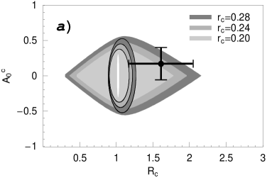
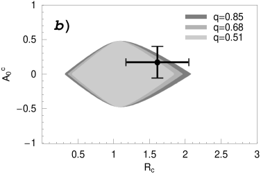
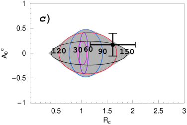
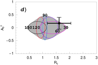
Figure 1: Allowed regions in the $R_{\rm c}$–$A_{0}^{\rm c}$ plane: (a) corresponds to $0.20\leq r_{\rm c}\leq 0.28$ for $q=0.68$, and (b) to $0.51\leq q\leq 0.85$ for $r_{\rm c}=0.24$; the elliptical regions arise if we restrict $\gamma$ to the Standard-Model range (13). In (c) and (d), we show the contours for fixed values of $\gamma$ and $|\delta_{\rm c}|$, respectively ($r_{\rm c}=0.24$, $q=0.68$).

A similar exercise can also be performed for the mixed $B\to\pi K$ system. To this end, we have just to make appropriate replacements of variables in (14) and (15). Since electroweak penguins contribute only in colour-suppressed form to the corresponding decays, we may use $q\to 0$ in this case to a good approximation. Moreover, we have $r_{\rm c,n}\to r$, where the determination of $r$ requires the use of arguments related to factorization [7, 9] to fix the colour-allowed amplitude $|T|$, or the measurement of $B_{s}\to\pi^{\pm}K^{\mp}$ [42], which is related to $B_{d}\to\pi^{\mp}K^{\pm}$ through the $U$-spin flavour symmetry of strong interactions. The presently most refined theoretical study of $r$ can be found in [41], using the QCD factorization approach. In our analysis, we shall consider the range $0.14\leq r\leq 0.26$. Since we have to make use of dynamical arguments to fix $q$ and $r$ in the case of the mixed $B\to\pi K$ system, it is not as clean as the charged and neutral $B\to\pi K$ systems.

   

   

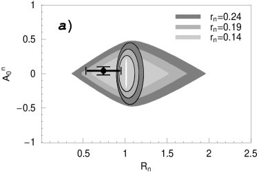
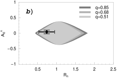
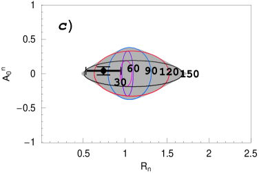
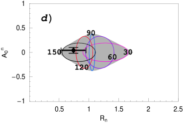
Figure 2: Allowed regions in the $R_{\rm n}$–$A_{0}^{\rm n}$ plane: (a) corresponds to $0.14\leq r_{\rm n}\leq 0.24$ for $q=0.68$, and (b) to $0.51\leq q\leq 0.85$ for $r_{\rm n}=0.19$; the elliptical regions arise if we restrict $\gamma$ to the Standard-Model range (13). In (c) and (d), we show the contours for fixed values of $\gamma$ and $|\delta_{\rm n}|$, respectively ($r_{\rm n}=0.19$, $q=0.68$).

2.2 Numerical Analysis

In Figs. 1 and 2, we show the allowed regions in observable space of the charged and neutral $B\to\pi K$ systems, respectively. The crosses correspond to the averages of the experimental results given in Tables 1 and 2, and the elliptical regions arise, if we restrict $\gamma$ to the Standard-Model range specified in (13). The labels of the contours in (c) refer to the values of $\gamma$ for $-180^{\circ}\leq\delta_{\rm c,n}\leq+180^{\circ}$, and those of (d) to the values of $|\delta_{\rm c,n}|$ for $0^{\circ}\leq\gamma\leq 180^{\circ}$. Looking at these figures, we observe that the experimental data fall pretty well into the regions, which are implied by the Standard-Model expressions (14) and (15). However, the data points do not favour the restricted region, which arises if we constrain $\gamma$ to its Standard-Model range (13). To be more specific, let us consider the contours shown in (c) and (d), allowing us to read off the preferred values for $\gamma$ and $|\delta_{\rm c,n}|$ directly from the measured observables. In the charged $B\to\pi K$ system, the $B$-factory data point towards values for $\gamma$ larger than $90^{\circ}$, and $|\delta_{\rm c}|$ smaller than $90^{\circ}$. In the case of the neutral $B\to\pi K$ system, the data are also in favour of $\gamma>90^{\circ}$, but prefer $|\delta_{\rm n}|$ to be larger than $90^{\circ}$. These features were also pointed out in [14]; in Figs. 1 and 2, we can see them directly from the data points. If future measurements should stabilize at such a picture, we would have a very exciting situation, since values for $\gamma$ larger than $90^{\circ}$ would be in conflict with the Standard-Model range (13), and the strong phases $\delta_{\rm c}$ and $\delta_{\rm n}$ are expected to be of the same order of magnitude; factorization would correspond to values around $0^{\circ}$. A possible explanation for such discrepancies would be given by large new-physics contributions to the electroweak penguin sector [14]. However, it should be kept in mind that we may also have “anomalously” large flavour-symmetry breaking effects. A detailed recent analysis of the allowed regions in parameter space of $\gamma$ and $\delta_{\rm c,n}$ that are implied by the present $B\to\pi K$ data can be found in [43], where also very restricted ranges for $R_{\rm c,n}$ were obtained by contraining $\gamma$ to its Standard-Model expectation. Another $B\to\pi K$ study was recently performed in [44], where the $R_{\rm(c)}$ were calculated for given values of $A_{0}^{\rm(c)}$ as functions of $\gamma$, and were compared with the present $B$-factory data.

   

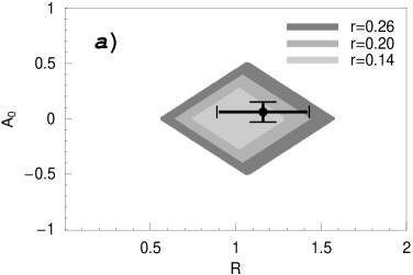
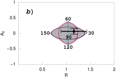
Figure 3: Allowed regions in the $R$–$A_{0}$ plane: (a) corresponds to $0.14\leq r\leq 0.26$ for $q=0$. In (b), we have chosen $r=0.20$ to show the contours for fixed values of $\gamma$ and $\delta$, which are identical for $q=0$. Moreover, we obtain the same contours for $\gamma\to 180^{\circ}-\gamma$.

In Fig. 3, we show the allowed region in observable space of the mixed $B\to\pi K$ system. Here the crosses represent again the averages of the experimental $B$-factory results. Since the expressions for $R$ and $A_{0}$ are symmetric with respect to an interchange of $\gamma$ and $\delta$ for $q=0$, the contours for fixed values of $\gamma$ and $\delta$ are identical in this limit. Moreover, we obtain the same contours for $\gamma\to 180^{\circ}-\gamma$. The experimental data fall well into the allowed region, but do not yet allow us to draw any further conclusions. In the charged and neutral $B\to\pi K$ systems, the situation appears to be much more exciting.

Let us now turn to the main aspect of our analysis, the $B_{d}\to\pi^{+}\pi^{-}$, $B_{s}\to K^{+}K^{-}$ system. In our original paper [16], we have addressed these modes only briefly, giving in particular a three-dimensional allowed region in the space of the CP asymmetries ${\cal A}_{\rm CP}^{\rm dir}(B_{s}\to K^{+}K^{-})$, ${\cal A}_{\rm CP}^{\rm mix}(B_{s}\to K^{+}K^{-})$ and ${\cal A}_{\rm CP}^{\rm dir}(B_{d}\to\pi^{+}\pi^{-})$. Here we follow [26], and use the CP-averaged $B_{d}\to\pi^{\mp}K^{\pm}$ branching ratio as an additional input to explore separately the allowed regions in the space of the CP-violating $B_{d}\to\pi^{+}\pi^{-}$ and $B_{s}\to K^{+}K^{-}$ observables, as well as contraints on $\gamma$. The experimental situation has improved significantly since [16] and [26] were written, pointing now to an interesting picture, although the uncertainties are still too large to draw definite conclusions. However, these uncertainties will be reduced considerably in the future due to the continuing efforts at the $B$ factories. Once the $B_{s}\to K^{+}K^{-}$ mode is accessible at hadronic $B$ experiments, more refined studies will be possible. In the LHC era, the physics potential of the $B_{d}\to\pi^{+}\pi^{-}$, $B_{s}\to K^{+}K^{-}$ system can then be fully exploited. In this paper, we point out that the Standard-Model range in $B_{s}\to K^{+}K^{-}$ observable space is very constrainted, thereby providing a narrow target range for these experiments.

3 Basic Features of the $B_{d}\to\pi^{+}\pi^{-}$, $B_{s}\to K^{+}K^{-}$ System and the Connection with $B_{d}\to\pi^{\mp}K^{\pm}$

3.1 Amplitude Parametrizations and Observables

The decay $B_{d}^{0}\to\pi^{+}\pi^{-}$ originates from $\overline{b}\to\overline{d}$ quark-level transitions. Within the Standard Model, it can be parametrized as follows [45]:

$$A(B_{d}^{0}\to\pi^{+}\pi^{-})=\lambda_{u}^{(d)}\left(A_{\rm CC}^{u}+A_{\rm pen}^{u}\right)+\lambda_{c}^{(d)}A_{\rm pen}^{c}+\lambda_{t}^{(d)}A_{\rm pen}^{t}\,,$$ (22)

where $A_{\rm CC}^{u}$ is due to “current–current” contributions, the amplitudes $A_{\rm pen}^{j}$ describe “penguin” topologies with internal $j$ quarks ($j\in\{u,c,t\})$, and the

$$\lambda_{j}^{(d)}\equiv V_{jd}V_{jb}^{\ast}$$ (23)

are the usual CKM factors. Employing the unitarity of the CKM matrix and the Wolfenstein parametrization [37], generalized to include non-leading terms in $\lambda\equiv|V_{us}|=0.222$ [46], we arrive at [15]

$$A(B_{d}^{0}\to\pi^{+}\pi^{-})={\cal C}\left(e^{i\gamma}-de^{i\theta}\right),$$ (24)

where

$${\cal C}\equiv\lambda^{3}AR_{b}\left(A_{\rm CC}^{u}+A_{\rm pen}^{ut}\right),$$ (25)

with $A_{\rm pen}^{ut}\equiv A_{\rm pen}^{u}-A_{\rm pen}^{t}$, and

$$de^{i\theta}\equiv\frac{1}{R_{b}}\left(\frac{A_{\rm pen}^{ct}}{A_{\rm CC}^{u}+A_{\rm pen}^{ut}}\right).$$ (26)

The quantity $A_{\rm pen}^{ct}$ is defined in analogy to $A_{\rm pen}^{ut}$, $A\equiv|V_{cb}|/\lambda^{2}=0.832\pm 0.033$, and $R_{b}$ was already introduced in (20). The “penguin parameter” $de^{i\theta}$ measures – sloppily speaking – the ratio of the $B_{d}\to\pi^{+}\pi^{-}$ “penguin” to “tree” contributions.

Using the Standard-Model parametrization (24), we obtain [15]

$${\cal A}_{\rm CP}^{\rm dir}(B_{d}\to\pi^{+}\pi^{-}) = -\left[\frac{2d\sin\theta\sin\gamma}{1-2d\cos\theta\cos\gamma+d^{2}}\right]$$ (27)

$${\cal A}_{\rm CP}^{\rm mix}(B_{d}\to\pi^{+}\pi^{-}) = \frac{\sin(\phi_{d}+2\gamma)-2d\cos\theta\sin(\phi_{d}+\gamma)+d^{2}\sin\phi_{d}}{1-2d\cos\theta\cos\gamma+d^{2}},$$ (28)

where $\phi_{d}=2\beta$ can be determined with the help of (3), yielding the twofold solution given in (5). Strictly speaking, mixing-induced CP violation in $B_{d}\to J/\psi K_{\rm S}$ probes $\phi_{d}+\phi_{K}$, where $\phi_{K}$ is related to the weak $K^{0}$–$\overline{K^{0}}$ mixing phase and is negligibly small in the Standard Model. However, due to the small value of the CP-violating parameter $\varepsilon_{K}$ of the neutral kaon system, $\phi_{K}$ can only be affected by very contrived models of new physics [47].

In the case of $B_{s}\to K^{+}K^{-}$, we have [15]

$$A(B_{s}^{0}\to K^{+}K^{-})=\left(\frac{\lambda}{1-\lambda^{2}/2}\right){\cal C}^{\prime}\left[e^{i\gamma}+\left(\frac{1-\lambda^{2}}{\lambda^{2}}\right)d^{\prime}e^{i\theta^{\prime}}\right],$$ (29)

where

$${\cal C}^{\prime}\equiv\lambda^{3}A\,R_{b}\left(A_{\rm CC}^{u^{\prime}}+A_{\rm pen}^{ut^{\prime}}\right)$$ (30)

and

$$d^{\prime}e^{i\theta^{\prime}}\equiv\frac{1}{R_{b}}\left(\frac{A_{\rm pen}^{ct^{\prime}}}{A_{\rm CC}^{u^{\prime}}+A_{\rm pen}^{ut^{\prime}}}\right)$$ (31)

correspond to (25) and (26), respectively. The primes remind us that we are dealing with a $\overline{b}\to\overline{s}$ transition. Introducing

$$\tilde{d}^{\prime}\equiv\frac{d^{\prime}}{\epsilon}\quad\mbox{with}\quad\epsilon\equiv\frac{\lambda^{2}}{1-\lambda^{2}},$$ (32)

we obtain [15]

$${\cal A}_{\rm CP}^{\rm dir}(B_{s}\to K^{+}K^{-}) = \frac{2\tilde{d}^{\prime}\sin\theta^{\prime}\sin\gamma}{1+2\tilde{d}^{\prime}\cos\theta^{\prime}\cos\gamma+\tilde{d}^{\prime 2}}$$ (33)

$${\cal A}_{\rm CP}^{\rm mix}(B_{s}\to K^{+}K^{-}) = \frac{\sin(\phi_{s}+2\gamma)+2\tilde{d}^{\prime}\cos\theta^{\prime}\sin(\phi_{s}+\gamma)+\tilde{d}^{\prime 2}\sin\phi_{s}}{1+2\tilde{d}^{\prime}\cos\theta^{\prime}\cos\gamma+\tilde{d}^{\prime 2}},$$ (34)

where the $B^{0}_{s}$–$\overline{B^{0}_{s}}$ mixing phase

$$\phi_{s}=-2\lambda^{2}\eta$$ (35)

is negligibly small in the Standard Model. Using the range for the Wolfenstein parameter $\eta$ following from the fits of the unitarity triangle [30] yields $\phi_{s}={\cal O}(-2^{\circ})$. Experimentally, this phase can be probed nicely through $B_{s}\to J/\psi\phi$, which allows an extraction of $\phi_{s}$ also if this phase should be sizeable due to new-physics contributions to $B^{0}_{s}$–$\overline{B^{0}_{s}}$ mixing [47]–[49].

It should be emphasized that (27), (28) and (33), (34) are completely general parametrizations of the CP-violating $B_{d}\to\pi^{+}\pi^{-}$ and $B_{s}\to K^{+}K^{-}$ observables, respectively, relying only on the unitarity of the CKM matrix. If we assume that $\phi_{s}$ is negligibly small, as in the Standard Model, these four observables depend on the four hadronic parameters $d$, $\theta$, $d^{\prime}$ and $\theta^{\prime}$, as well as on the two weak phases $\gamma$ and $\phi_{d}$. Consequently, we have not sufficient information to determine these quantities. However, since $B_{d}\to\pi^{+}\pi^{-}$ is related to $B_{s}\to K^{+}K^{-}$ through an interchange of all down and strange quarks, the $U$-spin flavour symmetry of strong interactions implies

$$de^{i\theta}=d^{\prime}e^{i\theta^{\prime}}.$$ (36)

Making use of this relation, the parameters $d$, $\theta$, $\gamma$ and $\phi_{d}$ can be determined from the CP-violating $B_{d}\to\pi^{+}\pi^{-}$, $B_{s}\to K^{+}K^{-}$ observables [15]. If we fix $\phi_{d}$ through (3), the use of the $U$-spin symmetry in the extraction of $\gamma$ can be minimized. Since $de^{i\theta}$ and $d^{\prime}e^{i\theta^{\prime}}$ are defined through ratios of strong amplitudes, the $U$-spin relation (36) is not affected by $U$-spin-breaking corrections in the factorization approximation [15], which gives us confidence in using this relation.

3.2 Constraints on Penguin Parameters

In order to constrain the hadronic penguin parameters through the CP-averaged $B_{d}\to\pi^{+}\pi^{-}$ and $B_{s}\to K^{+}K^{-}$ branching ratios, it is useful to introduce the following quantity [26]:

$$H\equiv\frac{1}{\epsilon}\,\left|\frac{{\cal C}^{\prime}}{{\cal C}}\right|^{2}\left[\frac{M_{B_{d}}}{M_{B_{s}}}\,\frac{\Phi(M_{K}/M_{B_{s}},M_{K}/M_{B_{s}})}{\Phi(M_{\pi}/M_{B_{d}},M_{\pi}/M_{B_{d}})}\,\frac{\tau_{B_{s}}}{\tau_{B_{d}}}\right]\left[\frac{\mbox{BR}(B_{d}\to\pi^{+}\pi^{-})}{\mbox{BR}(B_{s}\to K^{+}K^{-})}\right],$$ (37)

where

$$\Phi(x,y)\equiv\sqrt{\left[1-(x+y)^{2}\right]\left[1-(x-y)^{2}\right]}$$ (38)

denotes the usual two-body phase-space function. The branching ratio BR$(B_{s}\to K^{+}K^{-})$ can be extracted from the “untagged” $B_{s}\to K^{+}K^{-}$ rate [15], where no rapid oscillatory $\Delta M_{s}t$ terms are present [50]. In the strict $U$-spin limit, we have

$$|{\cal C}^{\prime}|=|{\cal C}|.$$ (39)

Corrections to this relation can be calculated using “factorization”, which yields

$$\left|\frac{{\cal C}^{\prime}}{{\cal C}}\right|_{\rm fact}=\,\frac{f_{K}}{f_{\pi}}\frac{F_{B_{s}K}(M_{K}^{2};0^{+})}{F_{B_{d}\pi}(M_{\pi}^{2};0^{+})}\left(\frac{M_{B_{s}}^{2}-M_{K}^{2}}{M_{B_{d}}^{2}-M_{\pi}^{2}}\right),$$ (40)

where the form factors $F_{B_{s}K}(M_{K}^{2};0^{+})$ and $F_{B_{d}\pi}(M_{\pi}^{2};0^{+})$ parametrize the hadronic quark-current matrix elements $\langle K^{-}|(\bar{b}u)_{\rm V-A}|B^{0}_{s}\rangle$ and $\langle\pi^{-}|(\bar{b}u)_{\rm V-A}|B^{0}_{d}\rangle$, respectively [51]. Employing (24) and (29) gives

$$H=\frac{1-2d\cos\theta\cos\gamma+d^{2}}{\epsilon^{2}+2\epsilon d^{\prime}\cos\theta^{\prime}\cos\gamma+d^{\prime 2}}.$$ (41)

Let us note that there is also an interesting relation between $H$ and the corresponding direct CP asymmetries [15]:

$$H=-\left(\frac{d\sin\theta}{d^{\prime}\sin\theta^{\prime}}\right)\frac{1}{\epsilon}\left[\frac{{\cal A}_{\rm CP}^{\rm dir}(B_{s}\to K^{+}K^{-})}{{\cal A}_{\rm CP}^{\rm dir}(B_{d}\to\pi^{+}\pi^{-})}\right].$$ (42)

Relations of this kind are a general feature of $U$-spin-related $B$ decays [52].

As can be seen in (41), if we use the $U$-spin relation (36), $H$ allows us to determine

$$C\equiv\cos\theta\cos\gamma$$ (43)

as a function of $d$ [26]:

$$C=\frac{a-d^{2}}{2bd},$$ (44)

where

$$a\equiv\frac{1-\epsilon^{2}H}{H-1}\qquad\mbox{and}\qquad b\equiv\frac{1+\epsilon H}{H-1}.$$ (45)

Since $C$ is the product of two cosines, it has to satisfy the relation $-1\leq C\leq+1$, implying the following allowed range for $d$:

$$\frac{1-\epsilon\sqrt{H}}{1+\sqrt{H}}\leq d\leq\frac{1+\epsilon\sqrt{H}}{|1-\sqrt{H}|}.$$ (46)

An alternative derivation of this range, which holds for $H<1/\epsilon^{2}=372$, was given in [53].

3.3 Connection with $B_{d}\to\pi^{\mp}K^{\pm}$

As we have already noted, experimental data on $B_{s}\to K^{+}K^{-}$ are not yet available. However, since $B_{s}\to K^{+}K^{-}$ and $B_{d}\to\pi^{\mp}K^{\pm}$ differ only in their spectator quarks, we have

$${\cal A}_{\rm CP}^{\rm dir}(B_{s}\to K^{+}K^{-})\approx{\cal A}_{\rm CP}^{\rm dir}(B_{d}\to\pi^{\mp}K^{\pm})$$ (47)

$$\mbox{BR}(B_{s}\to K^{+}K^{-})\approx\mbox{BR}(B_{d}\to\pi^{\mp}K^{\pm})\,\frac{\tau_{B_{s}}}{\tau_{B_{d}}},$$ (48)

and obtain

$$H\approx\frac{1}{\epsilon}\left(\frac{f_{K}}{f_{\pi}}\right)^{2}\left[\frac{\mbox{BR}(B_{d}\to\pi^{+}\pi^{-})}{\mbox{BR}(B_{d}\to\pi^{\mp}K^{\pm})}\right]=\left\{\begin{array}[]{ll}7.3\pm 2.9&\mbox{(CLEO \cite[cite]{[\@@bibref{}{CLEO-BpiK}{}{}]})}\\ 9.0\pm 1.5&\mbox{(BaBar \cite[cite]{[\@@bibref{}{BaBar-Bpipi-new}{}{}]})}\\ 8.5\pm 3.7&\mbox{(Belle \cite[cite]{[\@@bibref{}{belle-BpiK}{}{}]}),}\end{array}\right.$$ (49)

yielding the average

$$H=8.3\pm 1.6,$$ (50)

which has been calculated by simply adding the errors in quadrature. Clearly, the advantage of (49) is that it allows us to determine $H$ from the $B$-factory data, without a measurement of $B_{s}\to K^{+}K^{-}$. On the other hand – in contrast to (37) – this relation relies not only on $SU(3)$ flavour-symmetry arguments, but also on a certain dynamical assumption. The point is that $B_{s}\to K^{+}K^{-}$ receives also contributions from “exchange” and “penguin annihilation” topologies, which are absent in $B_{d}\to\pi^{\mp}K^{\pm}$. It is usually assumed that these contributions play a minor rôle [6]. However, they may be enhanced through certain rescattering effects [39]. The importance of the “exchange” and “penguin annihilation” topologies contributing to $B_{s}\to K^{+}K^{-}$ can be probed – in addition to (47) and (48) – with the help of $B_{s}\to\pi^{+}\pi^{-}$. The naïve expectation for the corresponding branching ratio is ${\cal O}(10^{-8})$; a significant enhancement would signal that the “exchange” and “penguin annihilation” topologies cannot be neglected. At run II of the Tevatron, a first measurement of $B_{s}\to K^{+}K^{-}$ will be possible.

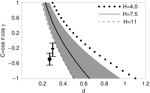
Figure 4: The dependence of $C=\cos\theta\cos\gamma$ on $d$ for values of $H$ lying within (51). The “circle” and “square” with error bars represent the predictions of the QCD factorization [41] and PQCD [54] approaches, respectively, for the Standard-Model range of $\gamma$ given in (13). The shaded region corresponds to a variation of $\xi$ within $[0.8,1.2]$ for $H=7.5$.

In Fig. 4, which is an update of a plot given in [26], we show the dependence of $C$ on $d$ arising from (44) for various values of $H$. Because of possible uncertainties arising from non-factorizable corrections to (40) and the dynamical assumptions employed in (48), we consider the range

$$H=7.5\pm 3.5,$$ (51)

which is more conservative than (50). The “circle” and “square” in Fig. 4 represent the predictions for $de^{i\theta}$ presented in [41] and [54], which were obtained within the QCD factorization [40] and perturbative hard-scattering (or “PQCD”) [55] approaches, respectively. The “error bars” correspond to the Standard-Model range (13) for $\gamma$, whereas the circle and square are evaluated for $\gamma=60^{\circ}$. The shaded region in Fig. 4 corresponds to a variation of

$$\xi\equiv d^{\prime}/d$$ (52)

within $[0.8,1.2]$ for $H=7.5$. As noted in [26], the impact of a sizeable phase difference

$$\Delta\theta\equiv\theta^{\prime}-\theta,$$ (53)

representing the second kind of possible corrections to (36), is very small in this case.

Looking at Fig. 4, we observe that the experimental values for $H$ imply a rather restricted range for $d$, satisfying $0.2\mathrel{\hbox{\hbox to0.0pt{\hbox{\lower 4.0pt\hbox{$\sim$}}\hss}\hbox{$<$}}}d\mathrel{\hbox{\hbox to0.0pt{\hbox{\lower 4.0pt\hbox{$\sim$}}\hss}\hbox{$<$}}}1$. Moreover, the curves are not in favour of an interpretation of the QCD factorization and PQCD predictions for $de^{i\theta}$ within the Standard Model. In the latter case, the prediction is somewhat closer to the “experimental” curves. This feature is due to the fact that the CP-conserving strong phase $\theta$ may deviate significantly from its trivial value of $180^{\circ}$ in PQCD, $\theta_{\rm PQCD}=101^{\circ}\sim 130^{\circ}$, which is in contrast to the result of QCD factorization, yielding $\theta_{\rm QCDF}=185^{\circ}\sim 193^{\circ}$. As a result, the PQCD approach may accommodate large direct CP violation in $B_{d}\to\pi^{+}\pi^{-}$, up to the $50\%$ level [54], whereas QCD factorization prefers smaller asymmetries, i.e. below the $20\%$ level [41]. In a recent paper [56], it was noted that higher-order corrections to QCD factorization in $B\to\pi K,\pi\pi$ decays may enhance the corresponding predictions for the CP-conserving strong phases, thereby also enhancing the direct CP asymmetries. Let us also note that the authors of [57], investigating the impact of “charming” penguins on the QCD factorization approach for $B\to\pi K,\pi\pi$ modes, found values for ${\cal A}_{\rm CP}^{\rm dir}(B_{d}\to\pi^{+}\pi^{-})$ as large as ${\cal O}(50\%)$.

Interestingly, the Belle measurement given in (6) is actually in favour of large direct CP violation in $B_{d}\to\pi^{+}\pi^{-}$. Since we restrict $\gamma$ to the range $[0^{\circ},180^{\circ}]$ in our analysis, the negative sign of ${\cal A}_{\rm CP}^{\rm dir}(B_{d}\to\pi^{+}\pi^{-})$ implies

$$0^{\circ}<\theta<180^{\circ},$$ (54)

as can be seen in (27). Interestingly, $\theta_{\rm PQCD}$ is consistent with this range, i.e. the sign of the prediction for ${\cal A}_{\rm CP}^{\rm dir}(B_{d}\to\pi^{+}\pi^{-})$ agrees with the one favoured by Belle, whereas $\theta_{\rm QCDF}$ lies outside, yielding the opposite sign for the direct CP asymmetry.

Another interesting observation in Fig. 4 is that the theoretical predictions for the hadronic parameter $de^{i\theta}$ could be brought to agreement with the experimental curves for values of $\gamma$ larger than $90^{\circ}$ [26]. In this case, the sign of $\cos\gamma$ becomes negative, and the circle and square in Fig. 4 move to positive values of $C$. Arguments for $\gamma>90^{\circ}$ using $B\to PP$, $PV$ and $VV$ decays were also given in [58]. Moreover, as we have seen in Subsection 2.2, the charged and neutral $B\to\pi K$ systems may point towards such values for $\gamma$ as well [14].

The constraints arising from $H$ have also implications for the CP-violating observables of the $B_{d}\to\pi^{+}\pi^{-}$, $B_{s}\to K^{+}K^{-}$ ($B_{d}\to\pi^{\mp}K^{\pm}$) decays. In [26], upper bounds on the corresponding direct CP asymmetries and an allowed range for ${\cal A}_{\rm CP}^{\rm mix}(B_{d}\to\pi^{+}\pi^{-})$ were derived as functions of $\gamma$. Here we use the information provided by $H$ to explore the allowed regions in the space of the CP-violating $B_{d}\to\pi^{+}\pi^{-}$ and $B_{s}\to K^{+}K^{-}$ observables, as well as constraints on $\gamma$. For other recent analyses of these decays, we refer the reader to [31, 44, 59].

4 Allowed Regions in $B_{d}\to\pi^{+}\pi^{-}$ Observable Space

4.1 General Formulae

The starting point of our considerations is the general expression (28) for ${\cal A}_{\rm CP}^{\rm mix}(B_{d}\to\pi^{+}\pi^{-})$, which allows us to eliminate the strong phase $\theta$ in (27), yielding

$${\cal A}_{\rm CP}^{\rm dir}(B_{d}\to\pi^{+}\pi^{-})=\mp\left[\frac{\sqrt{4d^{2}-\left(u+vd^{2}\right)^{2}}\sin\gamma}{(1-u\cos\gamma)+(1-v\cos\gamma)d^{2}}\right],$$ (55)

where $u$ and $v$ are defined as in [15]:

$$u\equiv\frac{{\cal A}_{\rm CP}^{\rm mix}(B_{d}\to\pi^{+}\pi^{-})-\sin(\phi_{d}+2\gamma)}{{\cal A}_{\rm CP}^{\rm mix}(B_{d}\to\pi^{+}\pi^{-})\cos\gamma-\sin(\phi_{d}+\gamma)}$$ (56)

$$v\equiv\frac{{\cal A}_{\rm CP}^{\rm mix}(B_{d}\to\pi^{+}\pi^{-})-\sin\phi_{d}}{{\cal A}_{\rm CP}^{\rm mix}(B_{d}\to\pi^{+}\pi^{-})\cos\gamma-\sin(\phi_{d}+\gamma)}.$$ (57)

It should be emphasized that (55) is valid exactly. If we use the $U$-spin relation (36), we may also eliminate $\theta$ through ${\cal A}_{\rm CP}^{\rm mix}(B_{d}\to\pi^{+}\pi^{-})$ in (41). Taking into account, moreover, the possible corrections to (36) through (52) and (53), we obtain the following expression for $d^{2}$:

$$d^{2}=\frac{AB+(2-uv)S^{2}\pm|S|\sqrt{4AB-(Av+Bu)^{2}+4(1-uv)S^{2}}}{B^{2}+v^{2}S^{2}},$$ (58)

where

$$A \equiv 1-\epsilon^{2}H-u\left(1+\epsilon\xi H\cos\Delta\theta\right)\cos\gamma$$ (59)

$$B \equiv \xi^{2}H-1+v\left(1+\epsilon\xi H\cos\Delta\theta\right)\cos\gamma$$ (60)

$$S \equiv \epsilon\xi H\cos\gamma\sin\Delta\theta.$$ (61)

In the limit of $\Delta\theta=0^{\circ}$, (58) simplifies to

$$\left.d^{2}\right|_{\Delta\theta=0^{\circ}}=\frac{A}{B}=\frac{1-\epsilon^{2}H-u\left(1+\epsilon\xi H\right)\cos\gamma}{\xi^{2}H-1+v\left(1+\epsilon\xi H\right)\cos\gamma}.$$ (62)

If we now insert $d^{2}$ thus determined into (55), we may calculate ${\cal A}_{\rm CP}^{\rm dir}(B_{d}\to\pi^{+}\pi^{-})$ as a function of $\gamma$ for given values of $H$, ${\cal A}_{\rm CP}^{\rm mix}(B_{d}\to\pi^{+}\pi^{-})$ and $\phi_{d}$. It is an easy exercise to show that (55) and (58) are invariant under the following replacements:

$$\phi_{d}\to 180^{\circ}-\phi_{d},\quad\gamma\to 180^{\circ}-\gamma,$$ (63)

which will have important consequences below.

In the following, we assume that $\phi_{d}$ and $H$ are known from (5) and (49), respectively. If we then vary $\gamma$ within $[0^{\circ},180^{\circ}]$ for each value of ${\cal A}_{\rm CP}^{\rm mix}(B_{d}\to\pi^{+}\pi^{-})\in[-1,+1]$, we obtain an allowed range in the ${\cal A}_{\rm CP}^{\rm mix}(B_{d}\to\pi^{+}\pi^{-})$–${\cal A}_{\rm CP}^{\rm dir}(B_{d}\to\pi^{+}\pi^{-})$ plane. Restricting $\gamma$ to (13), a more constrained region arises. The allowed range in the ${\cal A}_{\rm CP}^{\rm mix}(B_{d}\to\pi^{+}\pi^{-})$–${\cal A}_{\rm CP}^{\rm dir}(B_{d}\to\pi^{+}\pi^{-})$ plane can be obtained alternatively by eliminating $d$ through $H$ in (27) and (28), and then varying $\gamma$ and $\theta$ within the ranges of $[0^{\circ},180^{\circ}]$ and $[-180^{\circ},+180^{\circ}]$, respectively.

A different approach to analyse the situation in the ${\cal A}_{\rm CP}^{\rm mix}(B_{d}\to\pi^{+}\pi^{-})$–${\cal A}_{\rm CP}^{\rm dir}(B_{d}\to\pi^{+}\pi^{-})$ plane was employed in [31]. In this paper, the parameter $de^{i\theta}$ introduced in (26) is written as $-P_{\pi\pi}/T_{\pi\pi}$, where the magnitude of the “penguin” amplitude $P_{\pi\pi}$ is fixed through the CP-averaged branching ratio of the penguin-dominated decay $B^{\pm}\to\pi^{\pm}K$ with the help of $SU(3)$ flavour-symmetry arguments and plausible dynamical assumptions, concerning the neglect of an annihilation amplitude ${\cal A}$. In order to deal with $T_{\pi\pi}\propto(A^{u}_{\rm CC}+A^{ut}_{\rm pen})$, the penguin piece $A^{ut}_{\rm pen}$ is neglected, and the magnitude of the “tree” amplitude $A^{u}_{\rm CC}$ is estimated using factorization and data on $B\to\pi\ell\nu$, yielding $d\equiv|P_{\pi\pi}/T_{\pi\pi}|=0.276\pm 0.064$ [44]. Moreover, using the unitarity relation $\gamma=180^{\circ}-\alpha-\beta$ to eliminate $\gamma$, the observables ${\cal A}_{\rm CP}^{\rm mix}(B_{d}\to\pi^{+}\pi^{-})$ and ${\cal A}_{\rm CP}^{\rm dir}(B_{d}\to\pi^{+}\pi^{-})$ are expressed in terms of $\alpha$, $\beta$ and $P_{\pi\pi}/T_{\pi\pi}$. Fixing $\beta$ to be equal to the “Standard-Model” solution of $26^{\circ}$ implied by $B_{d}\to J/\psi K_{\rm S}$, and estimating $|P_{\pi\pi}/T_{\pi\pi}|$ as sketched above, ${\cal A}_{\rm CP}^{\rm mix}(B_{d}\to\pi^{+}\pi^{-})$ and ${\cal A}_{\rm CP}^{\rm dir}(B_{d}\to\pi^{+}\pi^{-})$ depend only on $\alpha$ and $\theta$. For each given value of $\alpha$, the variation of $\theta$ within the range $[-180^{\circ},+180^{\circ}]$ specifies then a contour in the ${\cal A}_{\rm CP}^{\rm mix}(B_{d}\to\pi^{+}\pi^{-})$–${\cal A}_{\rm CP}^{\rm dir}(B_{d}\to\pi^{+}\pi^{-})$ plane, holding within the Standard Model.

In our analysis, we prefer to use $H$ as an additional observable to deal with the penguin contributions, i.e. with the parameter $de^{i\theta}$, since we have then not to make a separation between $P_{\pi\pi}$ and $T_{\pi\pi}$, and have in particular not to rely on the naïve factorization approach to estimate the overall magnitude of $T_{\pi\pi}$, which is governed by colour-allowed tree-diagram-like processes, but may also be affected by penguin contributions. In our approach, factorization is only used to include $SU(3)$-breaking effects. Concerning the parametrization in terms of weak phases, we prefer to use $\gamma$ and the general $B^{0}_{d}$–$\overline{B^{0}_{d}}$ mixing phase $\phi_{d}$, since the results for the former quantity can then be compared easily with constraints from other processes, whereas the latter can anyway be fixed straighforwardly through mixing-induced CP violation in $B_{d}\to J/\psi K_{\rm S}$ up to a twofold ambiguity, also if there should be CP-violating new-physics contributions to $B^{0}_{d}$–$\overline{B^{0}_{d}}$ mixing. This way, we obtain an interesting connection between the two solutions for $\phi_{d}$ and the allowed ranges for $\gamma$, as we will see in the next subsection.

4.2 Numerical Analysis

In Fig. 5, we show the situation in the ${\cal A}_{\rm CP}^{\rm mix}(B_{d}\to\pi^{+}\pi^{-})$–${\cal A}_{\rm CP}^{\rm dir}(B_{d}\to\pi^{+}\pi^{-})$ plane for the central values of the two solutions for $\phi_{d}$ given in (5), and values of $H$ lying within (51). The impact of the present experimental uncertainty of $\phi_{d}$ is already very small, and will become negligible in the future. In order to calculate Fig. 5, we have used, for simplicity, $\xi=1$ and $\Delta\theta=0^{\circ}$; the impact of variations of these parameters will be discussed in Subsection 4.3. The contours in Fig. 5 arise, if we fix $\gamma$ to the values specified through the labels, and vary $\theta$ within $[-180^{\circ},+180^{\circ}]$. We have also indicated the region which arises if we restrict $\gamma$ to the Standard-Model range (13). The crosses describe the experimental averages given in (8).

   

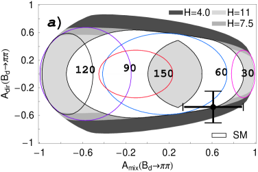
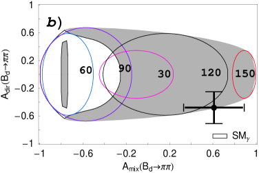
Figure 5: Allowed region in the ${\cal A}_{\rm CP}^{\rm mix}(B_{d}\to\pi^{+}\pi^{-})$–${\cal A}_{\rm CP}^{\rm dir}(B_{d}\to\pi^{+}\pi^{-})$ plane for (a) $\phi_{d}=51^{\circ}$ and various values of $H$, and (b) $\phi_{d}=129^{\circ}$ and $H=7.5$. The SM regions arise if we restrict $\gamma$ to (13) ($H=7.5$). We have also included the contours arising for various fixed values of $\gamma$.

We observe that the experimental averages overlap – within their uncertainties – nicely with the SM region for $\phi_{d}=51^{\circ}$, and point towards $\gamma\sim 50^{\circ}$. In this case, not only $\gamma$ would be in accordance with the results of the fits of the unitarity triangle [30], but also the $B^{0}_{d}$–$\overline{B^{0}_{d}}$ mixing phase $\phi_{d}$. On the other hand, for $\phi_{d}=129^{\circ}$, the experimental values favour $\gamma\sim 130^{\circ}$, and have essentially no overlap with the SM region. This feature is due to the symmetry relations given in (63). Since a value of $\phi_{d}=129^{\circ}$ would require CP-violating new-physics contributions to $B^{0}_{d}$–$\overline{B^{0}_{d}}$ mixing, also the $\gamma$ range in (13) may no longer hold, as it relies strongly on a Standard-Model interpretation of the experimental information on $B^{0}_{d,s}$–$\overline{B^{0}_{d,s}}$ mixing [30]. In particular, also values for $\gamma$ larger than $90^{\circ}$ could then in principle be accommodated. As we have noted in Subsection 3.3, theoretical analyses of $de^{i\theta}$ would actually favour values for $\gamma$ being larger than $90^{\circ}$, provided that the corresponding theoretical uncertainties are reliably under control, and that the $B_{d}\to\pi^{+}\pi^{-}$, $B_{s}\to K^{+}K^{-}$ system is still described by the Standard-Model parametrizations. In this case, (8) would point towards a $B^{0}_{d}$–$\overline{B^{0}_{d}}$ mixing phase of $129^{\circ}$, which would be a very exciting situation.

Consequently, it is very important to resolve the twofold ambiguity arising in (5) directly. To this end, $\cos\phi_{d}$ has to be measured as well. For the resolution of the discrete ambiguity, already a determination of the sign of $\cos\phi_{d}$ would be sufficient, where a positive result would imply that $\phi_{d}$ is given by $51^{\circ}$. There are several strategies on the market to accomplish this goal [49, 60]. Unfortunately, they are challenging from an experimental point of view and will require a couple of years of taking further data at the $B$ factories.

In order to put these observations on a more quantitative basis, we show in Fig. 6 the dependences of $|{\cal A}_{\rm CP}^{\rm dir}(B_{d}\to\pi^{+}\pi^{-})|$ on $\gamma$ for given values of ${\cal A}_{\rm CP}^{\rm mix}(B_{d}\to\pi^{+}\pi^{-})$. For the two solutions of $\phi_{d}$, an interesting difference arises, if we consider positive and negative values of the mixing-induced CP asymmetry, as done in (a), (b) and (c), (d), respectively, In the former case, we obtain the following excluded ranges for $\gamma$:

$$86^{\circ}\mathrel{\hbox{\hbox to0.0pt{\hbox{\lower 4.0pt\hbox{$\sim$}}\hss}\hbox{$<$}}}\gamma\mathrel{\hbox{\hbox to0.0pt{\hbox{\lower 4.0pt\hbox{$\sim$}}\hss}\hbox{$<$}}}140^{\circ}\,(\phi_{d}=51^{\circ}),\quad 40^{\circ}\mathrel{\hbox{\hbox to0.0pt{\hbox{\lower 4.0pt\hbox{$\sim$}}\hss}\hbox{$<$}}}\gamma\mathrel{\hbox{\hbox to0.0pt{\hbox{\lower 4.0pt\hbox{$\sim$}}\hss}\hbox{$<$}}}94^{\circ}\,(\phi_{d}=129^{\circ}).$$ (64)

Consequently, for $\phi_{d}=51^{\circ}$, we can conveniently accommodate the Standard-Model range (13), in contrast to the situation for $\phi_{d}=129^{\circ}$. On the other hand, if we consider negative values of ${\cal A}_{\rm CP}^{\rm mix}(B_{d}\to\pi^{+}\pi^{-})$, we obtain the following allowed ranges for $\gamma$:

$$50^{\circ}\mathrel{\hbox{\hbox to0.0pt{\hbox{\lower 4.0pt\hbox{$\sim$}}\hss}\hbox{$<$}}}\gamma\mathrel{\hbox{\hbox to0.0pt{\hbox{\lower 4.0pt\hbox{$\sim$}}\hss}\hbox{$<$}}}160^{\circ}\,(\phi_{d}=51^{\circ}),\quad 20^{\circ}\mathrel{\hbox{\hbox to0.0pt{\hbox{\lower 4.0pt\hbox{$\sim$}}\hss}\hbox{$<$}}}\gamma\mathrel{\hbox{\hbox to0.0pt{\hbox{\lower 4.0pt\hbox{$\sim$}}\hss}\hbox{$<$}}}130^{\circ}\,(\phi_{d}=129^{\circ}).$$ (65)

In this case, both ranges would contain (13), and the situation would not be as exciting as for a positive value of ${\cal A}_{\rm CP}^{\rm mix}(B_{d}\to\pi^{+}\pi^{-})$. These features can be understood in a rather transparent manner from the extremal values for ${\cal A}_{\rm CP}^{\rm mix}(B_{d}\to\pi^{+}\pi^{-})$ derived in [26].

In Fig. 6, we have also included bands, which are due to the present experimental averages given in (8). Interestingly, a positive value of ${\cal A}_{\rm CP}^{\rm mix}(B_{d}\to\pi^{+}\pi^{-})$ is now favoured by the data. From the overlap of the ${\cal A}_{\rm CP}^{\rm mix}(B_{d}\to\pi^{+}\pi^{-})$ and $|{\cal A}_{\rm CP}^{\rm dir}(B_{d}\to\pi^{+}\pi^{-})|$ bands we obtain the following solutions for $\gamma$:

$$28^{\circ}\mathrel{\hbox{\hbox to0.0pt{\hbox{\lower 4.0pt\hbox{$\sim$}}\hss}\hbox{$<$}}}\gamma\mathrel{\hbox{\hbox to0.0pt{\hbox{\lower 4.0pt\hbox{$\sim$}}\hss}\hbox{$<$}}}74^{\circ}\,(\phi_{d}=51^{\circ}),\quad 106^{\circ}\mathrel{\hbox{\hbox to0.0pt{\hbox{\lower 4.0pt\hbox{$\sim$}}\hss}\hbox{$<$}}}\gamma\mathrel{\hbox{\hbox to0.0pt{\hbox{\lower 4.0pt\hbox{$\sim$}}\hss}\hbox{$<$}}}152^{\circ}\,(\phi_{d}=129^{\circ}).$$ (66)

In the future, the experimental uncertainties will be reduced considerably, thereby providing much more stringent results for $\gamma$. Moreover, it should be emphasized that also $d$ can be determined with the help of (58). Going then back to (44), we may extract $\cos\theta$ as well, which allows an unambiguous determination of $\theta$ because of (54). Before we come back to this issue in Subsection 4.4, where we shall have a brief look at factorization and the discrete ambiguities arising typically in the extraction of $\gamma$ from the contours shown in Fig. 6, let us first turn to the uncertainties associated with the parameters $\xi$ and $\Delta\theta$.

   

   

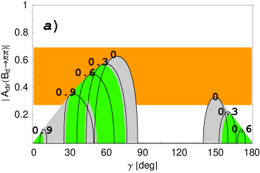
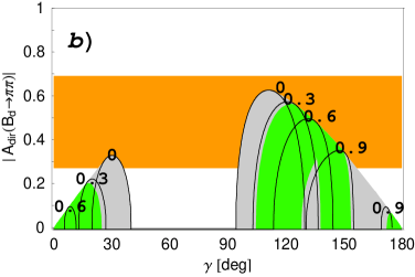
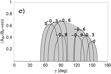
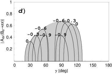
Figure 6: Dependence of $|{\cal A}_{\rm CP}^{\rm dir}(B_{d}\to\pi^{+}\pi^{-})|$ on $\gamma$ for various values of ${\cal A}_{\rm CP}^{\rm mix}(B_{d}\to\pi^{+}\pi^{-})$ in the case of $H=7.5$. In (a) and (b), we have chosen $\phi_{d}=51^{\circ}$ and $\phi_{d}=129^{\circ}$, respectively. The shaded region arises from a variation of ${\cal A}_{\rm CP}^{\rm mix}(B_{d}\to\pi^{+}\pi^{-})$ within $[0,+1]$. The corresponding plots for negative ${\cal A}_{\rm CP}^{\rm mix}(B_{d}\to\pi^{+}\pi^{-})$ are shown in (c) and (d) for $\phi_{d}=51^{\circ}$ and $\phi_{d}=129^{\circ}$, respectively. We have also included the bands arising from the experimental averages in (8).

   

   

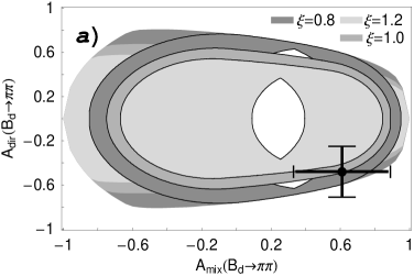
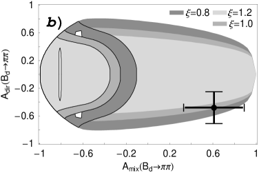
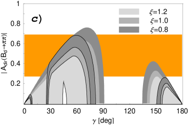
Figure 7: Impact of a variation of $\xi$ within $[0.8,1.2]$ for $H=7.5$ on (a), (b) the allowed ranges in the ${\cal A}_{\rm CP}^{\rm mix}(B_{d}\to\pi^{+}\pi^{-})$–${\cal A}_{\rm CP}^{\rm dir}(B_{d}\to\pi^{+}\pi^{-})$ plane, and (c), (d) the $\gamma$–$|{\cal A}_{\rm CP}^{\rm dir}(B_{d}\to\pi^{+}\pi^{-})|$ plane for positive values of ${\cal A}_{\rm CP}^{\rm mix}(B_{d}\to\pi^{+}\pi^{-})$, as explained in the text. We have used $\phi_{d}=51^{\circ}$ and $\phi_{d}=129^{\circ}$ in (a), (c) and (b), (d), respectively.

4.3 Sensitivity on $\xi$ and $\Delta\theta$

In the numerical analysis discussed in Subsection 4.2, we have used $\xi=1$ and $\Delta\theta=0^{\circ}$. Let us now investigate the sensitivity of our results on deviations of $\xi$ from 1, and sizeable values of $\Delta\theta$. The formulae given in Subsection 4.1 take into account these parameters exactly, thereby allowing us to study their effects straightforwardly. It turns out that the impact of $\Delta\theta$ is very small, even for values as large as $\pm 20^{\circ}$. Consequently, the most important effects are due to the parameter $\xi$. In Fig. 7, we use $H=7.5$ to illustrate the impact of a variation of $\xi$ within the range $[0.8,1.2]$: in (a) and (b), we show the allowed region in the ${\cal A}_{\rm CP}^{\rm mix}(B_{d}\to\pi^{+}\pi^{-})$–${\cal A}_{\rm CP}^{\rm dir}(B_{d}\to\pi^{+}\pi^{-})$ plane for $\phi_{d}=51^{\circ}$ and $129^{\circ}$, respectively, including also the regions, which arise if we restrict $\gamma$ to the Standard-Model range (13). In (c) and (d), we show the corresponding situation in the $\gamma$–$|{\cal A}_{\rm CP}^{\rm dir}(B_{d}\to\pi^{+}\pi^{-})|$ plane for positive values of ${\cal A}_{\rm CP}^{\rm mix}(B_{d}\to\pi^{+}\pi^{-})$. Here we have also included the bands arising from the present experimental values for CP violation in $B_{d}\to\pi^{+}\pi^{-}$. We find that a variation of $\xi$ within $[0.8,1.2]$ affects our result (66) for $\gamma$ as follows:

$$(28\pm 2)^{\circ}\mathrel{\hbox{\hbox to0.0pt{\hbox{\lower 4.0pt\hbox{$\sim$}}\hss}\hbox{$<$}}}\gamma\mathrel{\hbox{\hbox to0.0pt{\hbox{\lower 4.0pt\hbox{$\sim$}}\hss}\hbox{$<$}}}(74\pm 6)^{\circ}\,(\phi_{d}=51^{\circ}),\quad(106\pm 6)^{\circ}\mathrel{\hbox{\hbox to0.0pt{\hbox{\lower 4.0pt\hbox{$\sim$}}\hss}\hbox{$<$}}}\gamma\mathrel{\hbox{\hbox to0.0pt{\hbox{\lower 4.0pt\hbox{$\sim$}}\hss}\hbox{$<$}}}(152\pm 2)^{\circ}\,(\phi_{d}=129^{\circ}).$$ (67)

For future reduced experimental uncertainties of $|{\cal A}_{\rm CP}^{\rm dir}(B_{d}\to\pi^{+}\pi^{-})|$, also the holes in Figs. 7 (c) and (d) may have an impact on $\gamma$, excluding certain values. The impact of the hole is increasing for decreasing values of $\xi$. In Figs. 7 (c) and (d), only the smallest holes for $\xi=1.2$ are shown, whereas those corresponding $\xi=1.0$ and $\xi=0.8$ are hidden.

The range for $\xi$ considered in Figs. 4 and 7 appears rather conservative to us, since (36) is not affected by $U$-spin-breaking corrections within the factorization approach, in contrast to (39), as can be seen in (40). Non-factorizable corrections to the latter relation would show up as a systematic shift of $H$, and could be taken into account straightforwardly in our formalism.

   

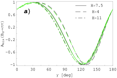
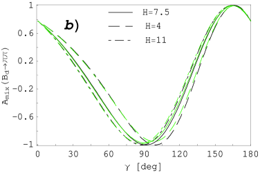
Figure 8: The dependence of ${\cal A}_{\rm CP}^{\rm mix}(B_{d}\to\pi^{+}\pi^{-})$ on $\gamma$ arising from (71) with (68) for $c=c^{\prime}=1$. In (a) and (b), we have chosen $\phi_{d}=51^{\circ}$ and $\phi_{d}=129^{\circ}$, respectively. We have also indicated the small shifts of the curves for a variation of $\theta=\theta^{\prime}$ between $160^{\circ}$ and $200^{\circ}$.

4.4 Comments on Factorization and Discrete Ambiguities

As we have noted in the introduction, the present BaBar and Belle measurements of CP violation in $B_{d}\to\pi^{+}\pi^{-}$ are not fully consistent with each other. Whereas Belle is in favour of very large CP asymmetries in this channel, the central values obtained by BaBar are close to zero. The Belle result and the average for ${\cal A}_{\rm CP}^{\rm dir}(B_{d}\to\pi^{+}\pi^{-})$ given in (8) cannot be accommodated within the factorization picture, predicting $\theta\sim 180^{\circ}$. On the other hand, this framework would still be consistent with BaBar. Let us therefore spend a few words on simplifications of the analysis given above that can be obtained by using a rather mild input from factorization.

If we look at (28) and (41), we observe that ${\cal A}_{\rm CP}^{\rm mix}(B_{d}\to\pi^{+}\pi^{-})$ and $H$ depend only on cosines of strong phases, which would be equal to $-1$ within factorization. In contrast to $\sin\theta$, the value of $\cos\theta$ is not very sensitive to deviations of $\theta$ from $\left.\theta\right|_{\rm fact}\sim 180^{\circ}$, i.e. to non-factorizable effects. Using (41), we obtain

$$d=\tilde{b}\cos\gamma+\sqrt{\tilde{a}+\left(\tilde{b}\cos\gamma\right)^{2}},$$ (68)

where

$$\tilde{a}\equiv\frac{1-\epsilon^{2}H}{\xi^{2}H-1},\quad\tilde{b}\equiv\frac{c+c^{\prime}\epsilon\xi H}{\xi^{2}H-1}$$ (69)

with

$$c\equiv-\cos\theta,\quad c^{\prime}\equiv-\cos\theta^{\prime}$$ (70)

are generalizations of $a$ and $b$ introduced in (45). The parameters $c$ and $c^{\prime}$ allow us to take into account deviations from the strict factorization limit, implying $c=c^{\prime}=1$. We may now calculate

$${\cal A}_{\rm CP}^{\rm mix}(B_{d}\to\pi^{+}\pi^{-})=\frac{\sin(\phi_{d}+2\gamma)+2dc\sin(\phi_{d}+\gamma)+d^{2}\sin\phi_{d}}{1+2dc\cos\gamma+d^{2}}$$ (71)

with the help of (68) as a function of $\gamma$.

In Fig. 8, we show the corresponding curves for various values of $H$ in the case of $c=c^{\prime}=1$; we have again to distinguish between (a) $\phi_{d}=51^{\circ}$, and (b) $\phi_{d}=129^{\circ}$. For a variation of $\theta=\theta^{\prime}$ between $160^{\circ}$ and $200^{\circ}$, we obtain very small shifts of these curves, as indicated in the figure. For ${\cal A}_{\rm CP}^{\rm mix}(B_{d}\to\pi^{+}\pi^{-})\sim 0$, as favoured by the present BaBar result, we would obtain

$$\gamma\sim 86^{\circ}\lor 160^{\circ}\,\,(\phi_{d}=51^{\circ}),\quad\gamma\sim 40^{\circ}\lor 130^{\circ}\,\,(\phi_{d}=129^{\circ}).$$ (72)

Using now once more (68) or the curves shown in Fig. 4 yields correspondingly

$$d\sim 0.4\lor 0.2\,\,(\phi_{d}=51^{\circ}),\quad d\sim 0.6\lor 0.3\,\,(\phi_{d}=129^{\circ}).$$ (73)

Since, as we have seen in Subsection 3.3, theoretical estimates prefer $d\sim 0.3$, the solutions for $\gamma$ larger than $90^{\circ}$ would be favoured. In (72) and (73), we obtain such solutions for both possible values of $\phi_{d}$.

The contours shown in Fig. 6 hold of course also in the case of ${\cal A}_{\rm CP}^{\rm dir}(B_{d}\to\pi^{+}\pi^{-})\sim 0$. However, we have then to deal with a fourfold discrete ambiguity in the extraction of $\gamma$ for each of the two possible values of $\phi_{d}$. Using the input about the cosines of strong phases from factorization, $c\sim c^{\prime}\sim 1$, these fourfold ambiguities are reduced for ${\cal A}_{\rm CP}^{\rm mix}(B_{d}\to\pi^{+}\pi^{-})\sim 0$ to the twofold ones given in (72). A similar comment applies also to other contours in Fig. 6.

Let us consider the contour corresponding to ${\cal A}_{\rm CP}^{\rm mix}(B_{d}\to\pi^{+}\pi^{-})=0.6$, which agrees with the central value in (8), to discuss this issue in more detail. For values of $|{\cal A}_{\rm CP}^{\rm dir}(B_{d}\to\pi^{+}\pi^{-})|\mathrel{\hbox{\hbox to0.0pt{\hbox{\lower 4.0pt\hbox{$\sim$}}\hss}\hbox{$>$}}}0.5$, we would obtain no solutions for $\gamma$. If, for instance, $|{\cal A}_{\rm CP}^{\rm dir}(B_{d}\to\pi^{+}\pi^{-})|$ should stabilize at 0.8, we would have an indication for new physics. In the case of $|{\cal A}_{\rm CP}^{\rm dir}(B_{d}\to\pi^{+}\pi^{-})|\sim 0.5$, the corresponding horizontal line touches the ${\cal A}_{\rm CP}^{\rm mix}(B_{d}\to\pi^{+}\pi^{-})=0.6$ contours, yielding $\gamma\sim 50^{\circ}$ and $130^{\circ}$ for $\phi_{d}=51^{\circ}$ and $\phi_{d}=129^{\circ}$, respectively. Moreover, $\theta\sim 90^{\circ}$ and $d\sim 0.4$ would be preferred in this case. For $\theta=\theta^{\prime}=90^{\circ}$, expression (41) implies

$$d=\sqrt{\frac{1-\epsilon^{2}H}{\xi^{2}H-1}},$$ (74)

which yields $d=0.39$ for $H=7.5$. It is amusing to note that $\theta=90^{\circ}$ and $d=0.39$ give for $(\gamma,\phi_{d})=(47^{\circ},51^{\circ})$ and $(133^{\circ},129^{\circ})$ the observables ${\cal A}_{\rm CP}^{\rm dir}(B_{d}\to\pi^{+}\pi^{-})=-0.49$ and ${\cal A}_{\rm CP}^{\rm mix}(B_{d}\to\pi^{+}\pi^{-})=+0.60$, which are both in excellent agreement with (8). If we reduce the value of $|{\cal A}_{\rm CP}^{\rm dir}(B_{d}\to\pi^{+}\pi^{-})|$ below 0.5, we obtain a twofold solution for $\gamma$, where the branches on the left-hand sides correspond to $0^{\circ}\mathrel{\hbox{\hbox to0.0pt{\hbox{\lower 4.0pt\hbox{$\sim$}}\hss}\hbox{$<$}}}\theta\mathrel{\hbox{\hbox to0.0pt{\hbox{\lower 4.0pt\hbox{$\sim$}}\hss}\hbox{$<$}}}90^{\circ}$ and those on the right-hand side to $90^{\circ}\mathrel{\hbox{\hbox to0.0pt{\hbox{\lower 4.0pt\hbox{$\sim$}}\hss}\hbox{$<$}}}\theta\mathrel{\hbox{\hbox to0.0pt{\hbox{\lower 4.0pt\hbox{$\sim$}}\hss}\hbox{$<$}}}180^{\circ}$. Consequently, the latter ones would be closer to factorization, and would also be in accordance with the PQCD analysis discussed in Subsection 3.3. As we have seen there, these theoretical predictions for $de^{i\theta}$ seem to favour $\gamma>90^{\circ}$, and would hence require that $\phi_{d}=129^{\circ}$ in Fig. 6. For values of $|{\cal A}_{\rm CP}^{\rm dir}(B_{d}\to\pi^{+}\pi^{-})|$ below 0.1, we would arrive at the fourfold ambiguities for $\gamma$ discussed above.

It will be very exciting to see in which direction the data will move. We hope that the discrepancy between the BaBar and Belle results will be resolved in the near future.

   

   

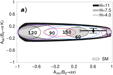
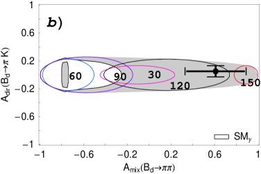
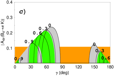
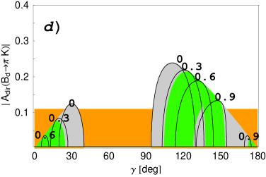
Figure 9: Correlations for the $B_{d}\to\pi^{+}\pi^{-}$, $B_{s}\to K^{+}K^{-}\approx B_{d}\to\pi^{\mp}K^{\pm}$ system: (a) and (b) are the allowed regions in the ${\cal A}_{\rm CP}^{\rm mix}(B_{d}\to\pi^{+}\pi^{-})$–${\cal A}_{\rm CP}^{\rm dir}(B_{d}\to\pi^{\mp}K^{\pm})$ plane for $\phi_{d}=51^{\circ}$ and $\phi_{d}=129^{\circ}$, respectively. In (c) and (d), we consider the $\gamma$–$|{\cal A}_{\rm CP}^{\rm dir}(B_{d}\to\pi^{\mp}K^{\pm})|$ plane for various values of ${\cal A}_{\rm CP}^{\rm mix}(B_{d}\to\pi^{+}\pi^{-})$ in the case of $\phi_{d}=51^{\circ}$ and $\phi_{d}=129^{\circ}$, respectively.

4.5 Correlations Between $B_{d}\to\pi^{+}\pi^{-}$ and $B_{d}\to\pi^{\mp}K^{\pm}$

Because of (42) and (47), it is also interesting to consider the CP asymmetry in $B_{d}\to\pi^{\mp}K^{\pm}$ decays instead of ${\cal A}_{\rm CP}^{\rm dir}(B_{d}\to\pi^{+}\pi^{-})$. The presently available $B$-factory measurements give

$${\cal A}_{\rm CP}^{\rm dir}(B_{d}\to\pi^{\mp}K^{\pm})=\left\{\begin{array}[]{ll}0.04\pm 0.16&\mbox{(CLEO \cite[cite]{[\@@bibref{}{CLEO-BpiK-CPV}{}{}]})}\\ 0.05\pm 0.06\pm 0.01&\mbox{(BaBar \cite[cite]{[\@@bibref{}{BaBar-Bpipi-new}{}{}]})}\\ 0.06\pm 0.08&\mbox{(Belle \cite[cite]{[\@@bibref{}{Belle-Bpipi}{}{}]}),}\end{array}\right.$$ (75)

yielding the average

$${\cal A}_{\rm CP}^{\rm dir}(B_{d}\to\pi^{\mp}K^{\pm})=0.05\pm 0.06.$$ (76)

On the other hand, inserting the experimental central values for ${\cal A}_{\rm CP}^{\rm dir}(B_{d}\to\pi^{+}\pi^{-})$ and $H$ into (47) yields ${\cal A}_{\rm CP}^{\rm dir}(B_{d}\to\pi^{\mp}K^{\pm})\sim 0.2$. In view of the present experimental uncertainties, this cannot be considered as a discrepancy. If we employ (42) and take into account (52) and (53), we obtain

$${\cal A}_{\rm CP}^{\rm dir}(B_{d}\to\pi^{\mp}K^{\pm})\approx{\cal A}_{\rm CP}^{\rm dir}(B_{s}\to K^{+}K^{-})$$

$$=-\epsilon\xi H\left[\cos\Delta\theta\pm\frac{\left(u+vd^{2}\right)\sin\Delta\theta}{\sqrt{4d^{2}-\left(u+vd^{2}\right)^{2}}}\right]{\cal A}_{\rm CP}^{\rm dir}(B_{d}\to\pi^{+}\pi^{-}),$$ (77)

where ${\cal A}_{\rm CP}^{\rm dir}(B_{d}\to\pi^{+}\pi^{-})$ is given by (55), with $d^{2}$ fixed through (58).

In Fig. 9, we collect the plots corresponding to those of the pure $B_{d}\to\pi^{+}\pi^{-}$ correlations given in Figs. 5 and 6: in (a) and (b), we show the allowed ranges in the ${\cal A}_{\rm CP}^{\rm mix}(B_{d}\to\pi^{+}\pi^{-})$–${\cal A}_{\rm CP}^{\rm dir}(B_{d}\to\pi^{\mp}K^{\pm})$ plane for $\phi_{d}=51^{\circ}$ and $\phi_{d}=129^{\circ}$, respectively, whereas the curves in (c) and (d) illustrate the corresponding situation in the $\gamma$–$|{\cal A}_{\rm CP}^{\rm dir}(B_{d}\to\pi^{\mp}K^{\pm})|$ plane for positive values of ${\cal A}_{\rm CP}^{\rm mix}(B_{d}\to\pi^{+}\pi^{-})$. We observe that the overlap of the experimental bands gives solutions for $\gamma$ that are consistent with (66), although we have now also two additional ranges for each $\phi_{d}$ due to the small central value of (76).

If we consider the allowed regions in observable space of the direct and mixing-induced CP asymmetries of the decay $B_{s}\to K^{+}K^{-}$, we obtain a very constrained situation. Let us next have a closer look at this particularly interesting transition.

5 Allowed Regions in $B_{s}\to K^{+}K^{-}$ Observable Space

5.1 General Formulae

From a conceptual point of view, the analysis of the decay $B_{s}\to K^{+}K^{-}$ is very similar to the one of $B_{d}\to\pi^{+}\pi^{-}$. If we use (34) to eliminate $\theta^{\prime}$ in (33), we arrive at

$${\cal A}_{\rm CP}^{\rm dir}(B_{s}\to K^{+}K^{-})=\pm\left[\frac{\sqrt{4\tilde{d}^{\prime 2}-\left(u^{\prime}+v^{\prime}\tilde{d}^{\prime 2}\right)^{2}}\sin\gamma}{(1-u^{\prime}\cos\gamma)+(1-v^{\prime}\cos\gamma)\tilde{d}^{\prime 2}}\right],$$ (78)

where $u^{\prime}$ and $v^{\prime}$ correspond to $u$ and $v$, respectively, and are given by

$$u^{\prime}\equiv\frac{{\cal A}_{\rm CP}^{\rm mix}(B_{s}\to K^{+}K^{-})-\sin(\phi_{s}+2\gamma)}{{\cal A}_{\rm CP}^{\rm mix}(B_{s}\to K^{+}K^{-})\cos\gamma-\sin(\phi_{s}+\gamma)}$$ (79)

$$v^{\prime}\equiv\frac{{\cal A}_{\rm CP}^{\rm mix}(B_{s}\to K^{+}K^{-})-\sin\phi_{s}}{{\cal A}_{\rm CP}^{\rm mix}(B_{s}\to K^{+}K^{-})\cos\gamma-\sin(\phi_{s}+\gamma)}.$$ (80)

In analogy to (55), (78) is also an exact expression. Making use of (36), the mixing-induced CP asymmetry ${\cal A}_{\rm CP}^{\rm mix}(B_{s}\to K^{+}K^{-})$ allows us to eliminate $\theta^{\prime}$ also in (41), thereby providing an expression for $\tilde{d}^{\prime 2}$. If we take into account, furthermore, (52) and (53), we obtain

$$\tilde{d}^{\prime 2}=\frac{A^{\prime}B^{\prime}+(2-u^{\prime}v^{\prime})S^{\prime 2}\pm|S^{\prime}|\sqrt{4A^{\prime}B^{\prime}-(A^{\prime}v^{\prime}+B^{\prime}u^{\prime})^{2}+4(1-u^{\prime}v^{\prime})S^{\prime 2}}}{B^{\prime 2}+v^{\prime 2}S^{\prime 2}},$$ (81)

with

$$A^{\prime} \equiv (\epsilon^{2}H-1)\xi^{2}-\epsilon\xi u^{\prime}(\cos\Delta\theta+\epsilon\xi H)\cos\gamma$$ (82)

$$B^{\prime} \equiv \epsilon\left[\epsilon\left(1-\xi^{2}H\right)+\xi v^{\prime}(\cos\Delta\theta+\epsilon\xi H)\cos\gamma\right]$$ (83)

$$S^{\prime} \equiv \epsilon\xi\cos\gamma\sin\Delta\theta.$$ (84)

In the limit of $\Delta\theta=0^{\circ}$, (81) simplifies to

$$\left.\tilde{d}^{\prime 2}\right|_{\Delta\theta=0^{\circ}}=\frac{A^{\prime}}{B^{\prime}}=\frac{(\epsilon^{2}H-1)\xi^{2}-\epsilon\xi u^{\prime}(1+\epsilon\xi H)\cos\gamma}{\epsilon\left[\epsilon\left(1-\xi^{2}H\right)+\xi v^{\prime}(1+\epsilon\xi H)\cos\gamma\right]}.$$ (85)

As in the case of $B_{d}\to\pi^{+}\pi^{-}$, (78) and (81) are invariant under the following symmetry transformation:

$$\phi_{s}\to 180^{\circ}-\phi_{s},\quad\gamma\to 180^{\circ}-\gamma.$$ (86)

Since $\phi_{s}$ is negligibly small in the Standard Model, these symmetry relations may only be of academic interest in the case of $B_{s}\to K^{+}K^{-}$. On the other hand, $\phi_{s}$ could in principle also be close to $180^{\circ}$. In this case, $B_{s}\to J/\psi\phi$ would not show CP-violating effects, as in the Standard Model. Strategies to distinguish between $\phi_{s}=0^{\circ}$ and $180^{\circ}$ were addressed in [49].

   

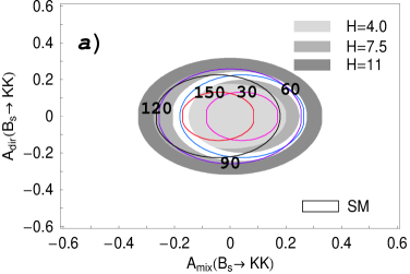
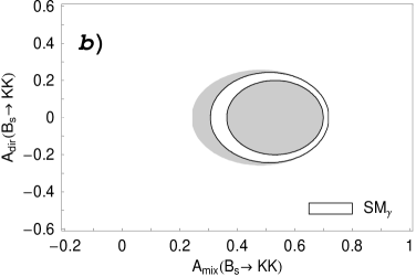
Figure 10: Allowed region in the ${\cal A}_{\rm CP}^{\rm mix}(B_{s}\to K^{+}K^{-})$–${\cal A}_{\rm CP}^{\rm dir}(B_{s}\to K^{+}K^{-})$ plane for (a) $\phi_{s}=0^{\circ}$ and various values of $H$, and (b) $\phi_{s}=30^{\circ}$, illustrating the impact of possible CP-violating new-physics contributions to $B^{0}_{s}$–$\overline{B^{0}_{s}}$ mixing. The SM regions arise if we restrict $\gamma$ to (13) ($H=7.5$). We have also included the contours corresponding to various fixed values of $\gamma$.

   

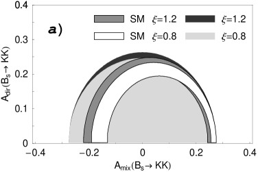
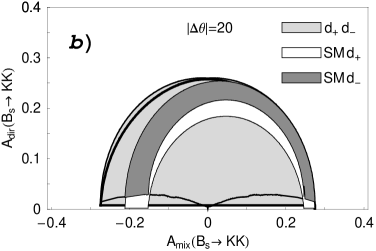
Figure 11: Impact of variations of (a) $\xi\in[0.8,1.2]$, and (b) $\Delta\theta\in[-20^{\circ},+20^{\circ}]$ on the allowed region in the ${\cal A}_{\rm CP}^{\rm mix}(B_{s}\to K^{+}K^{-})$–${\cal A}_{\rm CP}^{\rm dir}(B_{s}\to K^{+}K^{-})$ plane for $\phi_{s}=0^{\circ}$ ($H=7.5$). In (b), $d_{+}$ and $d_{-}$ correspond to the two solutions for $\tilde{d}^{\prime 2}$ arising in (81).

5.2 Numerical Analysis

In analogy to our study of $B_{d}\to\pi^{+}\pi^{-}$ in Section 4, we may now straightforwardly calculate the allowed region in the ${\cal A}_{\rm CP}^{\rm mix}(B_{s}\to K^{+}K^{-})$–${\cal A}_{\rm CP}^{\rm dir}(B_{s}\to K^{+}K^{-})$ plane. In Fig. 10, we show these correlations for (a) a negligible $B^{0}_{s}$–$\overline{B^{0}_{s}}$ mixing phase $\phi_{s}$, and (b) a value of $\phi_{s}=30^{\circ}$, illustrating the impact of possible CP-violating new-physics contributions to $B^{0}_{s}$–$\overline{B^{0}_{s}}$ mixing. We have also indicated the contours corresponding to various fixed values of $\gamma$, and the region, which arises if we restrict $\gamma$ to the Standard-Model range (13). In contrast to Fig. 5, the allowed region is now very constrained, thereby providing a narrow target range for run II of the Tevatron and the experiments of the LHC era. As we have seen in Subsection 4.5, the experimental constraints on ${\cal A}_{\rm CP}^{\rm dir}(B_{d}\to\pi^{\mp}K^{\pm})$ exclude already very large direct CP violation in this channel. Because of (47), we expect a similar situation in $B_{s}\to K^{+}K^{-}$, which is in accordance with Fig. 10. The allowed range for ${\cal A}_{\rm CP}^{\rm mix}(B_{s}\to K^{+}K^{-})$ may be shifted significantly through sizeable values of $\phi_{s}$. Such a scenario would be signaled independently through large CP-violating effects in the $B_{s}\to J/\psi\phi$ channel, which is very accessible at hadronic $B$ experiments. It is interesting to note that if the solution $\phi_{d}=129^{\circ}$ should actually be the correct one, it would be very likely to have also new-physics effects in $B^{0}_{s}$–$\overline{B^{0}_{s}}$ mixing. If we restrict $\gamma$ to the Standard-Model range (13), we even obtain a much more constrained allowed region, given by a rather narrow elliptical band.

The sensitivity of the allowed region in the ${\cal A}_{\rm CP}^{\rm mix}(B_{s}\to K^{+}K^{-})$–${\cal A}_{\rm CP}^{\rm dir}(B_{s}\to K^{+}K^{-})$ plane on variations of $\xi$ and $\Delta\theta$ within reasonable ranges is very small, as can be seen in Figs. 11 (a) and (b), respectively. In the latter figure, we consider $|\Delta\theta|=20^{\circ}$, and show explicitly the two solutions ($d_{+}$ and $d_{-}$) for $\tilde{d}^{\prime 2}$ arising in (81). As in Fig. 10, we consider again the whole range for $\gamma$, and its restriction to (13). The shifts with respect to the $\xi=1$, $\Delta\theta=0^{\circ}$ case are indeed small, as can be seen by comparing with rescaled Fig. 10 (a). Consequently, the main theoretical uncertainty of our predictions for the $B_{s}\to K^{+}K^{-}$ observable correlations is due to the determination of $H$.

It will be very exciting to see whether the measurements at run II of the Tevatron and at the experiments of the LHC era, where the physics potential of the $B_{s}\to K^{+}K^{-}$, $B_{d}\to\pi^{+}\pi^{-}$ system can be fully exploited, will actually hit the very constrained allowed region in observable space. In this case, it would be more advantageous not to use $H$ for the extraction of $\gamma$, but contours in the $\gamma$–$d^{\prime}$ and $\gamma$–$d$ planes, which can be fixed in a theoretically clean way through the CP-violating $B_{s}\to K^{+}K^{-}$ and $B_{d}\to\pi^{+}\pi^{-}$ observables, respectively [15]. Making then use of $d^{\prime}=\xi d$, $\gamma$ and the hadronic parameters $d$, $\theta$ and $\theta^{\prime}$ can be determined in a transparent manner. Concerning theoretical uncertainties, this is the cleanest way to extract information from the $B_{s}\to K^{+}K^{-}$, $B_{d}\to\pi^{+}\pi^{-}$ system. In particular, it does not rely on (40). It should be noted that this approach would also work, if $\phi_{s}$ turned out to be sizeable. This phase could then be determined through $B_{s}\to J/\psi\phi$ [48, 49].

5.3 Comments on Factorization

Using the same input from factorization as in Subsection 4.4, we obtain the following simplified expressions for the contours in the $\gamma$–$d^{\prime}$ and $\gamma$–$d$ planes:

$$d^{\prime}=\epsilon\left(\frac{c^{\prime}\pm\sqrt{c^{\prime 2}-u^{\prime}v^{\prime}}}{v^{\prime}}\right),\quad d=\frac{-c\pm\sqrt{c^{2}-uv}}{v},$$ (87)

where $u^{\prime}$, $v^{\prime}$ and $u$, $v$ are given in (79), (80) and (56), (57), respectively, and $c^{\prime}$ and $c$ are defined in (70). On the other hand, the general expressions derived in [15] that do not rely on factorization simplify for vanishing direct CP asymmetries in $B_{s}\to K^{+}K^{-}$ and $B_{d}\to\pi^{+}\pi^{-}$ as follows:

$$d^{\prime}=\epsilon\left|\frac{1\pm\sqrt{1-u^{\prime}v^{\prime}}}{v^{\prime}}\right|,\quad d=\left|\frac{-1\pm\sqrt{1-uv}}{v}\right|.$$ (88)

Consequently, since $d^{\prime}$ and $d$ are by definition positive parameters, the input from factorization would allow us to reduce the number of discrete ambiguities in this case. We have encountered a similar feature in our discussion of $B_{d}\to\pi^{+}\pi^{-}$ in Subsection 4.4. As noted in [15], in order to reduce the number of discrete ambiguities, also the contours in the $\gamma$–$d$ and $\gamma$–$d^{\prime}$ plane specified through (58) and (81), respectively, are very helpful.

   

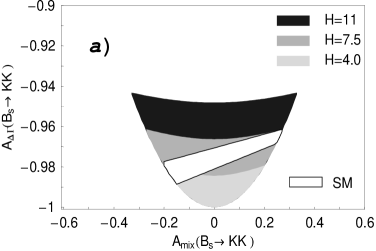
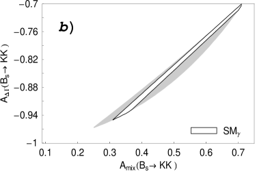
Figure 12: Allowed region in the ${\cal A}_{\rm CP}^{\rm mix}(B_{s}\to K^{+}K^{-})$–${\cal A}_{\Delta\Gamma}(B_{s}\to K^{+}K^{-})$ plane for (a) $\phi_{s}=0^{\circ}$ and various values of $H$, and (b) $\phi_{s}=30^{\circ}$, illustrating the impact of CP-violating new-physics contributions to $B^{0}_{s}$–$\overline{B^{0}_{s}}$ mixing. The SM regions arise if we restrict $\gamma$ to (13) ($H=7.5$).

5.4 The ${\cal A}_{\rm CP}^{\rm mix}(B_{s}\to K^{+}K^{-})$–${\cal A}_{\Delta\Gamma}(B_{s}\to K^{+}K^{-})$ Plane

Let us finally consider the observable ${\cal A}_{\Delta\Gamma}(B_{s}\to K^{+}K^{-})$ appearing in (1), which may be accessible due to a sizeable width difference $\Delta\Gamma_{s}$ of the $B_{s}$ system. Interestingly, this quantity may also be extracted from the “untagged” rate

$$\Gamma(B^{0}_{s}(t)\to K^{+}K^{-})+\Gamma(\overline{B^{0}_{s}}(t)\to K^{+}K^{-})\propto R_{\rm H}e^{-\Gamma_{\rm H}^{(s)}t}+R_{\rm L}e^{-\Gamma_{\rm L}^{(s)}t}$$ (89)

through

$${\cal A}_{\Delta\Gamma}(B_{s}\to K^{+}K^{-})=\frac{R_{\rm H}-R_{\rm L}}{R_{\rm H}+R_{\rm L}},$$ (90)

where $\Delta\Gamma_{s}\equiv\Gamma_{\rm H}^{(s)}-\Gamma_{\rm L}^{(s)}$ is negative in the Standard Model. Using parametrization (29), we obtain [15]

$${\cal A}_{\Delta\Gamma}(B_{s}\to K^{+}K^{-})=-\left[\frac{\cos(\phi_{s}+2\gamma)+2\tilde{d}^{\prime}\cos\theta^{\prime}\cos(\phi_{s}+\gamma)+\tilde{d}^{\prime 2}\cos\phi_{s}}{1+2\tilde{d}^{\prime}\cos\theta^{\prime}\cos\gamma+\tilde{d}^{\prime 2}}\right].$$ (91)

An important difference with respect to the direct CP asymmetry (33) is that – as in (34) – only $\cos\theta^{\prime}$ terms appear in this expression. Consequently, using the mixing-induced CP asymmetry ${\cal A}_{\rm CP}^{\rm mix}(B_{s}\to K^{+}K^{-})$ to eliminate $\cos\theta^{\prime}$, we arrive at

$${\cal A}_{\Delta\Gamma}(B_{s}\to K^{+}K^{-})=-\left[\frac{\cos(\phi_{s}+2\gamma)-u^{\prime}\cos(\phi_{s}+\gamma)+\left\{\cos\phi_{s}-v^{\prime}\cos(\phi_{s}+\gamma)\right\}\tilde{d}^{\prime 2}}{\left(1-u^{\prime}\cos\gamma\right)+\left(1-v^{\prime}\cos\gamma\right)\tilde{d}^{\prime 2}}\right].$$ (92)

In contrast to (78), no sign ambiguity appears in this expression; in the former, it is due to $\sin\theta^{\prime}=\pm\sqrt{1-\cos^{2}\theta^{\prime}}$. The square root in (78) ensures that

$$|\cos\theta^{\prime}|=\frac{|u^{\prime}+v^{\prime}\tilde{d}^{\prime 2}|}{2\tilde{d}^{\prime}}\leq 1.$$ (93)

If we fix $\tilde{d}^{\prime}$ through (81) and insert it into (92), we have to require, in addition, that this relation is satisfied. We may then perform an analysis similar to the one for the observables ${\cal A}_{\rm CP}^{\rm mix}(B_{s}\to K^{+}K^{-})$ and ${\cal A}_{\rm CP}^{\rm dir}(B_{s}\to K^{+}K^{-})$ given above.

In Fig. 12, we show the allowed region in the ${\cal A}_{\rm CP}^{\rm mix}(B_{s}\to K^{+}K^{-})$–${\cal A}_{\Delta\Gamma}(B_{s}\to K^{+}K^{-})$ plane for (a) the Standard-Model case of $\phi_{s}=0^{\circ}$, and (b) a value of $\phi_{s}=30^{\circ}$, illustrating the impact of possible new-physics contributions to $B^{0}_{s}$–$\overline{B^{0}_{s}}$ mixing. It should be noted that the width difference $\Delta\Gamma_{s}$ would be modified in the latter case as follows [49, 61]:

$$\Delta\Gamma_{s}=\Delta\Gamma_{s}^{\rm SM}\cos\phi_{s}.$$ (94)

As in Fig. 10, we have also included the regions, which arise if we restrict $\gamma$ to (13). We observe that ${\cal A}_{\Delta\Gamma}(B_{s}\to K^{+}K^{-})$ is highly constrained within the Standard Model, yielding

$$-1\mathrel{\hbox{\hbox to0.0pt{\hbox{\lower 4.0pt\hbox{$\sim$}}\hss}\hbox{$<$}}}{\cal A}_{\Delta\Gamma}(B_{s}\to K^{+}K^{-})\mathrel{\hbox{\hbox to0.0pt{\hbox{\lower 4.0pt\hbox{$\sim$}}\hss}\hbox{$<$}}}-0.95.$$ (95)

Moreover, it becomes evident that this observable may be affected significantly through sizeable values of $\phi_{s}$. Unfortunately, the width difference $|\Delta\Gamma_{s}|$ would be reduced in this case because of (94), thereby making measurements relying on a sizeable value of this quantity more difficult.

6 Conclusions and Outlook

In our paper, we have used recent experimental data to analyse allowed regions in the space of CP-violating $B\to\pi K$, $B_{d}\to\pi^{+}\pi^{-}$ and $B_{s}\to K^{+}K^{-}$ observables that arise within the Standard Model. The main results can be summarized as follows:

• As far as $B\to\pi K$ decays are concerned, the combinations of charged and neutral modes appear to be most exciting. We have presented contour plots, allowing us to read off the preferred ranges for $\gamma$ and strong phases $\delta_{\rm c,n}$ directly from the experimental data. The charged and neutral $B\to\pi K$ decays point both towards $\gamma>90^{\circ}$. On the other hand, they prefer $|\delta_{\rm c}|$ to be smaller than $90^{\circ}$, and $|\delta_{\rm n}|$ to be larger than $90^{\circ}$. This puzzling situation, which was also pointed out in [14], may be an indication of new-physics contributions to the electroweak penguin sector, but the uncertainties are still too large to draw definite conclusions. It should be kept in mind that we may also have “anomalously” large flavour-symmetry breaking effects.

• The present data on the CP-averaged $B_{d}\to\pi^{\mp}K^{\pm}$ and $B_{d}\to\pi^{+}\pi^{-}$ branching ratios allow us to obtain rather strong constraints on the penguin parameter $de^{i\theta}$. A comparison of the experimental curves with the most recent theoretical predictions for this parameter is not in favour of an interpretation within the Standard Model; comfortable agreement between theory and experiment could be achieved for values of $\gamma$ being larger than $90^{\circ}$.

• The constraints on $de^{i\theta}$ have interesting implications for the allowed region in the space of the mixing-induced and direct CP asymmetries of the decay $B_{d}\to\pi^{+}\pi^{-}$. Taking into account the first measurements of these observables at the $B$ factories, we arrive at the following picture:

  • For the $B^{0}_{d}$–$\overline{B^{0}_{d}}$ mixing phase $\phi_{d}=51^{\circ}$, the data favour a value of $\gamma\sim 50^{\circ}$. In this case, $\phi_{d}=2\beta$ and $\gamma$ would both agree with the results of the usual indirect fits of the unitarity triangle.

  • For the $B^{0}_{d}$–$\overline{B^{0}_{d}}$ mixing phase $\phi_{d}=180^{\circ}-51^{\circ}=129^{\circ}$, the data favour a value of $\gamma\sim 130^{\circ}$, i.e. larger than $90^{\circ}$. In this case, $\phi_{d}$ would require CP-violating new-physics contributions to $B^{0}_{d}$–$\overline{B^{0}_{d}}$ mixing, so that also the results of the usual indirect fits of the unitarity triangle for $\gamma$ may no longer hold.

  As we have noted above, $\gamma$ may actually be larger than $90^{\circ}$, which would then require the unconventional solution $\phi_{d}=129^{\circ}$. Consequently, it is very important to resolve the twofold ambiguity arising in the extraction of $\phi_{d}$ from ${\cal A}_{\rm CP}^{\rm mix}(B_{d}\to J/\psi K_{\rm S})=-\sin\phi_{d}$ directly through a measurement of the sign of $\cos\phi_{d}$.

• We have provided the formalism to take into account the parameters $\xi$ and $\Delta\theta$, affecting the theorectical accuracy of our approach, in an exact manner, and have studied their impact in detail.

• In the case of the decay $B_{s}\to K^{+}K^{-}$, we obtain a very constrained allowed region in the space of the corresponding CP-violating observables, thereby providing a narrow target range for run II of the Tevatron and the experiments of the LHC era. Here the impact of variations of $\xi$ and $\Delta\theta$ within reasonable ranges is practically negligible. On the basis of the present data on direct CP violation in $B_{d}\to\pi^{\mp}K^{\pm}$, we do not expect a very large value of ${\cal A}_{\rm CP}^{\rm dir}(B_{s}\to K^{+}K^{-})$, which is also in accordance with the allowed range derived in this paper. On the other hand, CP-violating new-physics contributions to $B^{0}_{s}$–$\overline{B^{0}_{s}}$ mixing may shift the range for ${\cal A}_{\rm CP}^{\rm mix}(B_{s}\to K^{+}K^{-})$ significantly.

• Using a moderate input from factorization about the cosines of CP-conserving strong phases, our analysis could be simplified, and the number of discrete ambiguities arising in the extraction of $\gamma$ could be reduced.

It will be very exciting to see in which direction the experimental results for the $B\to\pi K$, $B_{d}\to\pi^{+}\pi^{-}$ and $B_{s}\to K^{+}K^{-}$ observables will move. Unfortunately, the present measurements of the CP asymmetries in $B_{d}\to\pi^{+}\pi^{-}$ by BaBar and Belle are not fully consistent with each other. We hope that this discrepancy will be resolved soon. As we have pointed out in our analysis, we may obtain valuable insights into CP violation and the world of penguins from such measurements. A first analysis of $B_{s}\to K^{+}K^{-}$ will already be available at run II of the Tevatron, where $B^{0}_{s}$–$\overline{B^{0}_{s}}$ mixing should also be discovered, and $B_{s}\to J/\psi\phi$ may indicate a sizeable value of $\phi_{s}$. At the experiments of the LHC era, in particular LHCb and BTeV, the physics potential of the $B_{s}\to K^{+}K^{-}$, $B_{d}\to\pi^{+}\pi^{-}$ system to explore CP violation can then be fully exploited.

References

-
[1]
For reviews, see, for instance,
A.J. Buras, TUM-HEP-435-01 [hep-ph/0109197];
Y. Nir, WIS-18-01-DPP [hep-ph/0109090];
M. Gronau, TECHNION-PH-2000-30 [hep-ph/0011392];
J.L. Rosner, EFI-2000-47 [hep-ph/0011355];
R. Fleischer, DESY 00-170 [hep-ph/0011323]. -
[2]
A.B. Carter and A.I. Sanda,
Phys. Rev. Lett. 45 (1980) 952,
Phys. Rev. D23 (1981) 1567;
I.I. Bigi and A.I. Sanda, Nucl. Phys. B193 (1981) 85. - [3] BaBar Collaboration (B. Aubert et al.), Phys. Rev. Lett. 87 (2001) 091801.
- [4] Belle Collaboration (K. Abe et al.), Phys. Rev. Lett. 87 (2001) 091802.
- [5] M. Gronau, J.L. Rosner and D. London, Phys. Rev. Lett. 73 (1994) 21.
- [6] M. Gronau, O.F. Hernández, D. London and J.L. Rosner, Phys. Rev. D52 (1995) 6374.
- [7] R. Fleischer, Phys. Lett. B365 (1996) 399.
- [8] R. Fleischer and T. Mannel, Phys. Rev. D57 (1998) 2752.
- [9] M. Gronau and J.L. Rosner, Phys. Rev. D57 (1998) 6843.
- [10] R. Fleischer, Eur. Phys. J. C6 (1999) 451.
-
[11]
M. Neubert and J.L. Rosner,
Phys. Lett. B441 (1998) 403;
Phys. Rev. Lett. 81 (1998) 5076. - [12] M. Neubert, JHEP 9902 (1999) 014.
- [13] A.J. Buras and R. Fleischer, Eur. Phys. J. C11 (1999) 93.
- [14] A.J. Buras and R. Fleischer, Eur. Phys. J. C16 (2000) 97.
- [15] R. Fleischer, Phys. Lett. B459 (1999) 306.
- [16] R. Fleischer and J. Matias, Phys. Rev. D61 (2000) 074004.
-
[17]
R. Fleischer and T. Mannel, TTP-97-22,
[hep-ph/9706261];
D. Choudhury, B. Dutta and A. Kundu, Phys. Lett. B456 (1999) 185;
Y. Grossman, M. Neubert and A.L. Kagan, JHEP 9910 (1999) 029;
X.-G. He, C. Hsueh and J. Shi, Phys. Rev. Lett. 84 (2000) 18;
J. Matias, Phys. Lett. B520 (2001) 131. -
[18]
For a recent overview of the theoretical status of
, see
M. Beneke and A. Lenz, J. Phys. G27 (2001) 1219. - [19] BaBar Collaboration (B. Aubert et al.), BABAR-CONF-02/01 [hep-ex/0203007].
-
[20]
Talk by T. Karim (Belle Collaboration),
XXXVIIth Rencontres de Moriond, Electroweak Interactions and
Unified Theories, Les Arcs, France, 9–16 March 2002,
http://moriond.in2p3.fr/EW/2002/. - [21] CDF Collaboration (T. Affolder et al.), Phys. Rev. D61 (2000) 072005.
- [22] ALEPH Collaboration (R. Barate et al.), Phys. Lett. B492 (2000) 259.
- [23] R. Fleischer and T. Mannel, Phys. Lett. B506 (2001) 311.
-
[24]
K. Anikeev et al., FERMILAB-Pub-01/197
[hep-ph/0201071];
M. Tanaka (CDF Collaboration), Nucl. Instrum. Meth. A462 (2001) 165. - [25] P. Ball et al., CERN-TH-2000-101 [hep-ph/0003238].
- [26] R. Fleischer, Eur. Phys. J. C16 (2000) 87.
-
[27]
Talk by A. Farbin (BaBar Collaboration),
XXXVIIth Rencontres de Moriond, Electroweak Interactions and Unified
Theories, Les Arcs, France, 9–16 March 2002,
http://moriond.in2p3.fr/EW/2002/. - [28] Belle Collaboration (K. Abe et al.), Belle Preprint 2002-8 [hep-ex/0204002].
- [29] BaBar Collaboration (B. Aubert et al.), BABAR-CONF-01/05 [hep-ex/0107074].
-
[30]
For recent analyses, see A. Höcker et al.,
Eur. Phys. J. C21 (2001) 225;
M. Ciuchini et al., JHEP 0107 (2001) 013;
A. Ali and D. London, Eur. Phys. J. C18 (2001) 665. - [31] M. Gronau and J.L. Rosner, TECHNION-PH-2002-12 [hep-ph/0202170].
- [32] CLEO Collaboration (D. Cronin-Hennessy et al.), Phys. Rev. Lett. 85 (2000) 515.
- [33] BaBar Collaboration (B. Aubert et al.), Phys. Rev. Lett. 87 (2001) 151802.
- [34] Belle Collaboration (K. Abe et al.), Phys. Rev. Lett. 87 (2001) 101801.
- [35] CLEO Collaboration (S. Chen et al.), Phys. Rev. Lett. 85 (2000) 525.
- [36] Belle Collaboration (K. Abe et al.), Phys. Rev. D64 (2001) 071101.
- [37] L. Wolfenstein, Phys. Rev. Lett. 51 (1983) 1945.
- [38] Y. Grossman, B. Kayser and Y. Nir, Phys. Lett. B415 (1997) 90.
-
[39]
L. Wolfenstein,
Phys. Rev. D52 (1995) 537;
J.F. Donoghue et al., Phys. Rev. Lett. 77 (1996) 2178;
M. Neubert, Phys. Lett. B 424 (1998) 152;
J.-M. Gérard and J. Weyers, Eur. Phys. J. C7 (1999) 1;
A.J. Buras, R. Fleischer and T. Mannel, Nucl. Phys. B533 (1998) 3;
A.F. Falk, A.L. Kagan, Y. Nir and A.A. Petrov, Phys. Rev. D57 (1998) 4290;
R. Fleischer, Phys. Lett. B435 (1998) 221. - [40] M. Beneke, G. Buchalla, M. Neubert and C.T. Sachrajda, Phys. Rev. Lett. 83 (1999) 1914.
- [41] M. Beneke, G. Buchalla, M. Neubert and C.T. Sachrajda, Nucl. Phys. B606 (2001) 245.
- [42] M. Gronau and J.L. Rosner, Phys. Lett. B482 (2000) 71.
- [43] M. Bargiotti et al., hep-ph/0204029.
- [44] M. Gronau and J.L. Rosner, Phys. Rev. D65 (2002) 013004 [E: D65 (2002) 079901].
- [45] R. Fleischer, Int. J. Mod. Phys. A12 (1997) 2459.
- [46] A.J. Buras, M.E. Lautenbacher and G. Ostermaier, Phys. Rev. D50 (1994) 3433.
- [47] Y. Nir and D. Silverman, Nucl. Phys. B345 (1990) 301.
- [48] A.S. Dighe, I. Dunietz and R. Fleischer, Eur. Phys. J. C6 (1999) 647.
- [49] I. Dunietz, R. Fleischer and U. Nierste, Phys. Rev. D63 (2001) 114015.
- [50] I. Dunietz, Phys. Rev. D52 (1995) 3048.
- [51] M. Bauer, B. Stech and M. Wirbel, Z. Phys. C29 (1985) 637 and C34 (1987) 103.
- [52] M. Gronau, Phys. Lett. B492 (2000) 297.
- [53] D. Pirjol, Phys. Rev. D60 (1999) 054020.
- [54] A.I. Sanda and K. Ukai, DPNU-01-21 [hep-ph/0109001].
-
[55]
H.-n. Li and H.L. Yu,
Phys. Rev. D53 (1996) 2480;
Y.Y. Keum, H.-n. Li and A.I. Sanda, Phys. Lett. B504 (2001) 6,
Phys. Rev. D63 (2001) 054008;
Y.Y. Keum and H.-n. Li, Phys. Rev. D63 (2001) 074006. - [56] M. Neubert and B.D. Pecjak, JHEP 0202 (2002) 028.
- [57] M. Ciuchini et al., Phys. Lett. B515 (2001) 33.
-
[58]
W.S. Hou and K.C. Yang,
Phys. Rev. D61 (2000) 073014;
W.-S. Hou, J.G. Smith and F. Würthwein, NTU-HEP-99-25 [hep-ex/9910014]. - [59] M. Gronau and J.L. Rosner, TECHNION-PH-2002-14 [hep-ph/0203158].
-
[60]
Ya.I. Azimov, V.L. Rappoport and V.V. Sarantsev,
Z. Phys. A356 (1997) 437;
Y. Grossman and H.R. Quinn, Phys. Rev. D56 (1997) 7259;
A.S. Dighe, I. Dunietz and R. Fleischer, Phys. Lett. B433 (1998) 147;
J. Charles et al., Phys. Lett. B425 (1998) 375;
B. Kayser and D. London, Phys. Rev. D61 (2000) 116012;
H.R. Quinn, T. Schietinger, J.P. Silva, A.E. Snyder, Phys. Rev. Lett. 85 (2000) 5284. - [61] Y. Grossman, Phys. Lett. B380 (1996) 99.