Gauge Coupling Unification and Phenomenology
of Selected Orbifold 5D $N=1$ SUSY Models

Filipe Paccetti Correia^a, Michael G. Schmidt^a, Zurab Tavartkiladze^a,b

^aInstitut für Theoretische Physik, Universität Heidelberg, Philosophenweg 16,
D-69120 Heidelberg, Germany

^b Institute of Physics, Georgian Academy of Sciences, Tbilisi 380077, Georgia

We study gauge coupling unification and various phenomenological issues, such as baryon number conservation, the $\mu$ problem and neutrino anomalies, within SUSY 5D orbifold models. The 5D MSSM on an $S^{(1)}/Z_{2}$ orbifold with ’minimal’ field content does not lead to low scale unification, while some of its extensions can give unification near the multi TeV scale. Within the orbifold $SU(5)$ GUT, low scale unification can not be realized due to full $SU(5)$ multiplets participating in the renormalization above the compactification scale. As alternative examples, we construct 5D $N=1$ SUSY Pati-Salam $SU(4)_{c}\times SU(2)_{L}\times SU(2)_{R}\equiv G_{422}$ and flipped $SU(5)\times U(1)\equiv G_{51}$ GUTs [both maximal subgroups of $SO(10)$] on an $S^{(1)}/Z_{2}\times Z_{2}^{\prime}$ orbifold. New examples of low scale unifications within $G_{422}$ are presented. For $G_{51}$ the unification scale is shown to be necessarily close to $\sim 10^{16}$ GeV. The possible influence of brane couplings on the gauge coupling unification is also outlined. For the resolution of the various phenomenological problems extensions with a discrete ${\cal Z}$ symmetry turn out to be very effective.

1 Introduction: Old and new features of GUTs

The standard model of elementary particle physics (SM) gives an excellent explanation of all existing experimental data. However, there are quite strong theoretical motivations to believe that the SM is an effective theory of a more fundamental theory and that the gauge couplings of $SU(3)_{c}\times SU(2)_{L}\times U(1)_{Y}\equiv G_{321}$ have a common origin. The construction of grand unified theories (GUTs) [1], which unify $G_{321}$ gauge interactions in a single non Abelian group [$SU(5)$, $SO(10)$, $E_{6}$ etc], give an elegant explanation of charge quantization and also unify quark-lepton families. The idea of GUT got a great support from the fact that the three gauge couplings measured at that early times were indeed unifying at energies near $M_{G}\sim 10^{15}$ GeV [2]. Progress in measuring the strong gauge coupling and also the weak mixing angle $\sin^{2}\theta_{W}$ with higher accuracy has ruled out the minimal $SU(5)$ GUT [and also minimal $SO(10)$ without intermediate scale] from the viewpoint of coupling unification [3], [8]. However, the minimal supersymmetric extension of the standard model (MSSM) and also the minimal SUSY $SU(5)$ GUT [4](which except for GUT threshold corrections both have the same pattern of running of couplings below $M_{G}$) were giving values for the $\alpha_{3}(M_{Z})$ coupling [5]-[8] well within the experimental limits at that time. Indeed since SUSY theories stabilize hierarchies, for realistic model building supersymmetry might be the best way to proceed. It is assumed, that the SUSY breaking scale $m$ lies in a range $500$ GeV - few TeV and below this characteristic scale the theory is just the SM with minimal particle content except the Higgs sector, while above the $m$ scale the theory is supersymmetric. Despite these nice features of SUSY theories, there are various puzzles and problems, which are connected with SUSY GUTs and we will list some of them here.

(i) Baryon number violation is a particular feature of GUTs such as $SU(5)$, $SO(10)$. Since for SUSY GUTs the unification scale $M_{G}\simeq 2\cdot 10^{16}$ GeV is larger than for non SUSY GUTs, the gauge mediated $d=6$ nucleon decay is compatible with the latest SuperKamiokande (SK) limit $\tau_{N}\stackrel{{\scriptstyle>}}{{{}_{\sim}}}10^{33}$ yrs [9]. However, with SUSY there is a new source for nucleon decay through $d=5$ operators, which makes the minimal $SU(5)$ and $SO(10)$ scenarios incompatible [10] with SK data.

(ii) The unified multiplets of minimal $SU(5)$ lead to the wrong asymptotic mass relations $\hat{m}_{d}^{(0)}=\hat{m}_{e}^{(0)}$. In the minimal $SO(10)$ the situation is even worse, since $\hat{m}_{u}^{(0)}=\hat{m}_{d}^{(0)}=\hat{m}_{e}^{(0)}$ and $\hat{V}_{CKM}={\bf 1}$ is predicted.

(iii) The problem of doublet-triplet (DT) splitting in the Higgs supermultiplet still needs to be resolved. In GUTs, the MSSM Higgs doublets are usually accompanied by colored triplets. In order to maintain coupling unification and reasonably stable nucleons [triplets could induce nucleon decay through $d=5$ operators, see (i)], triplet components must be superheavy. So, one should provide a natural explanation of the fact that sometimes states (Higgs doublets and colored triplets) coming from the same GUT multiplet are split with a huge mass gap $M_{T}/M_{D}\geq 10^{13}$.

(iv) The spontaneous breaking of the GUT symmetry requires scalars in a high representation of the gauge group considered; thus the superpotential, responsible for symmetry breaking, contains many unknown parameters and usually looks rather complicated.

(v) The so-called $\mu$ problem exists even within the MSSM. 4D superpotential couplings allow a $Mh_{u}h_{d}$ term, where $h_{u}$, $h_{d}$ are the MSSM Higgs doublets and $M$ is some mass close to the cutoff scale of the theory. So, somehow large values for $\mu$($\sim M$) must be avoided. In order to have the desired electroweak symmetry breaking and a reasonable phenomenology, a $\mu$ term of the magnitude $\sim 500$ GeV - few TeV has to be generated in a good model (also within GUTs after solution of the DT splitting problem (iii) and having succeeded to obtain $\mu=0$ ).

(vi) Recent atmospheric [11] and solar [12] neutrino SK data have confirmed neutrino oscillations. The explanation of the atmospheric anomaly (by a characteristic mass squared scale $m^{2}_{atm}\sim 10^{-3}$ eV²) already forces us to step beyond the MSSM and the minimal SUSY $SU(5)$ (a neutrino mass $\sim 10^{-5}$ eV can be generated through Planck scale $d=5$ operators and can explain the solar anomaly through large angle vacuum oscillations. However, this solution is disfavored by the SK data). In order to have neutrinos with masses $0.1-1$ eV, the lepton number must be violated by a proper amount. This requires considering extensions of the MSSM and the minimal SUSY $SU(5)$. It would be most welcome if the considered model would contain a source for the needed lepton number violation.

(vii) Very accurate measurements of $\alpha_{3}(M_{Z})$ [9] already allow to judge whether a given GUT scenario is viable or not. Two loop renormalization studies of the MSSM (with all SUSY particles near the $M_{Z}$ scale) predict $\alpha_{3}(M_{Z})=0.126$ [13], which contradicts the experimental $\alpha_{3}^{exp}(M_{Z})=0.119\pm 0.002$ [9]. This situation can be improved either by pushing all SUSY particle masses up to the $\sim 3$ TeV mass scale [13], or by some GUT threshold corrections. With the latter the minimal SUSY $SU(5)$ does not give any promising results [14]. Comparing GUT scenarios, those would be considered more attractive which, without constraining the SUSY particle mass spectra, give acceptable values for the strong coupling.

On the theoretical side quite a few new possibilities have been found since the early days of GUTs and also the introduction of SUSY.

$\alpha$) String theory is primarily a theory of (super)gravity but it also contains in a less unique manner matter and gauge fields. It had an enormous effect on the taste of model builders although concrete phenomenological results are still not obvious. We particularly mention symmetry breaking mechanisms not requiring very high Higgs representations of the GUT gauge groups and a natural assignment of fundamental representation to matter. Also the possibility to calculate (in principle!) Yukawa couplings is very impressive. But unfortunately there is a huge and even increasing number of string vacua with (presently) no possibility to make a choice of one or the other except for phenomenological reasons. Still until recently [23] it was notoriously difficult to find a string model realization implementing the SM with three generations.

$\beta$) Extra dimensions: The Kaluza-Klein use of extra dimensions to be curled up one way or the other had several renaissances. Of course it is very tempting to obtain extra model informations from some extra dimensions - there is plenty of space in this dreamland, which can contain geometry/topology. In string theory extra dimensions are mandatory for consistency. A drawback then seems to be that such extra dimensions would show up only at the string scale which is normally identified with the Planck scale of our gravity. One then is led to talk about physics which presumably never will be tested in the laboratory. Recently it became a point of common interest whether the string scale might be as low as the TeV scale [24] still allowing for our gravity scale. In this case higher dimensions should show up soon in experiments [25].

$\gamma$) It was exciting news that dualities connect the various types of string theories [26]. The open string picture allows for $D$-branes which contain our 3-dimensional space but also allow for some extra dimensions which may be curled up or projected out in the case of intersecting branes. This version of string theory may be particularly appropriate also in the case of singular points of divided out symmetries for an approximation by a description in local quantum field theory language since there are no winding states.

In resolving problems (i)-(iv) of SUSY GUT scenarios the orbifold constructions seem to be very promising [15]-[22]. In the original paper of ref. [15], a five dimensional (5D) $N=1$ SUSY $SU(5)$ GUT on an $S^{(1)}/Z_{2}\times Z_{2}^{\prime}$ orbifold was considered. Due to this construction, it turns out that the problems (i)-(iv) can be resolved in a very natural way for a wide class of unified models [15]-[22], while (v)-(vii) still depend on peculiarities of the scenario considered and will be discussed in more detail below. Due to specific boundary conditions, it is possible to mod out selected sub-states from a given GUT representation. Through this self consistent procedure, it is possible to obtain the desired GUT symmetry breaking, nucleon stability and natural DT splitting.

In the last years, theories with extra dimensions have attracted great attention. Originally the main phenomenological motivation was the possibility to resolve the gauge hierarchy problem without supersymmetry. It was observed [27], that due to sufficiently large extra dimensions, it is possible to lower the fundamental scale $M_{f}$ even down to a few TeV (indeed, this can be an excellent starting point for understanding the electroweak scale), while the 4D Planck mass still has the required value $\sim 10^{19}$ GeV. Due to the large extra dimensions, Newton’s law could be modified at short distances where the behavior of gravity is still unknown and is studied in ongoing experiments [28]. Similarly and perhaps with a richer phenomenology [25], one can study the spectrum for scenarios with a string scale of a few TeV [24]. It turned out, that the presence of extra dimensions can play a crucial role also for obtaining low scale unification of gauge couplings [29]-[32] through power law running [33]. The construction of realistic GUT scenarios with low scale unification raises the hope that phenomenological implications can be detected. However, the orbifold GUT scenarios considered up to now do not allow for low scale unification [20], [21] because in these settings the GUT symmetry is restored at energies higher than the compactification scale. Thus full GUT multiplets [either of $SU(5)$ or $SO(10)$] will participate in the running and power law unification does not take place. Relatively low scales $\sim 10^{13-14}$ GeV are also preferable for lepton number violation. One way for obtaining unification on a scale much below $\sim 10^{16}$ GeV is to consider either GUT models with product groups or with (intermediate) stages of symmetry breaking - step by step compactification of more than one extra dimension. On the GUT scale $M_{G}$ a first step compactification ($1/R^{\prime}\sim M_{G}$) takes place and the unified group $G$ reduces to its subgroup $H$. In the second step compactification, whose scale $\mu_{0}=1/R$ is below $M_{G}$, the subgroup $H$ is broken. If $H$ is different from $SU(5)$ and if the states are non complete multiplets of $SU(5)$, then due to their contribution to the running between $\mu_{0}$ and $M_{G}$ there can appear power law unification on intermediate or low scales.

In this paper we consider 5D $N=1$ SUSY models with orbifold compactifications. We start our discussion with the standard model $G_{321}$ gauge group and an $S^{(1)}/Z_{2}$ orbifold. In order to have a model without the phenomenological problems (i)-(vi) [in this case except the (ii)-(iv) of course], we introduce a discrete ${\cal Z}$ symmetry which elegantly resolves problems (i), (v) and replacing matter $R$ parity allows for some lepton number violating couplings which can generate neutrino masses. Thus, (vi) also can be resolved. We confirm that, with the MSSM states plus appropriate Kaluza-Klein (KK) excitations, successful unification holds only for $1/R\simeq M_{G}\sim 10^{16}$ GeV. Low scale unification requires either some extensions [30], [31] or the existence of specific threshold corrections [32]. Similarly we can discuss 5D $N=1$ SUSY $SU(5)$ GUT on an $S^{(1)}/Z_{2}\times Z_{2}^{\prime}$ orbifold. In this setting the problems (ii)-(iv) are resolved naturally, while (i), (v) will again be resolved by introducing a discrete symmetry ${\cal Z}$. As far as the gauge coupling unification is concerned, all states including matter supermultiplets and their copies form full $SU(5)$ multiplets above the compactification scale. Because of this, low and intermediate scale unification can not take place. Then we address the question whether power law unification is possible or not (at low or intermediate scale) within the orbifold GUT construction. We emphasize the possibility of a so-called step by step compactification with an intermediate gauge group, different from the $SU(5)$ in structure and field content. This potentially allows for power law unification. Besides the latter a quite different and peculiar phenomenology can arise. To demonstrate this we consider Pati-Salam $SU(4)_{c}\times SU(2)_{L}\times SU(2)_{R}\equiv G_{422}$ [34] and flipped $SU(5)\times U(1)\equiv G_{51}$ GUTs. Both these gauge groups are maximal subgroups of $SO(10)$ [35], [36] and thus one could imagine that they are produced in a first step breaking of $SO(10)$ in six dimensions by the compactification of one dimension. Within 5D $N=1$ SUSY $G_{422}$ and $G_{51}$ models an extension with a discrete ${\cal Z}$ symmetry is needed for a simultaneous solution of the problems (i)-(vi). These models involve SM singlet right handed states which are necessary for the breaking of the rank and obtaining the $G_{321}$ gauge group. In combination with the ${\cal Z}$ symmetry, these singlet states also play a crucial role in understanding of problems (i), (v), (vi). They are also tied with lepton number violation and the generation of an intermediate symmetry breaking scale. The $G_{422}$ model allows to lower the unification scale not only down to intermediate scales, but even down to the multi TeV region. Differently, within $G_{51}$ the unification scale is close to $\sim 10^{16}$ GeV. The models considered have some peculiar phenomenological implications testable in the future.

The paper is organized as follows. In section 2 we present the main construction principles of the models considered. In section 3 we write the needed one loop renormalization-group equations (RGE). Using them we study gauge coupling unification within various models, in the presence of KK states. Sections 4 and 5 are devoted to the 5D orbifold $N=1$ SUSY $G_{321}$ and the $SU(5)$ models resp. In section 6 we discuss the issue of power law unification, within orbifold GUT scenarios, and outline the ways of its realization. In sections 7 and 8 Pati-Salam $G_{422}$ and flipped $SU(5)\times U(1)$ GUTs resp. are studied on an $S^{(1)}/Z_{2}\times Z_{2}^{\prime}$ orbifold. Finally discussions and conclusions are presented in section 9. The paper contains an Appendix A, in which the influence of some brane couplings on the gauge coupling running is estimated.

2 Construction principles of 5D SUSY
orbifold theories

In this section we present our construction principles of 5D SUSY theories. As we will see they are divided into two categories: principles which are related to the higher dimensionality and others which deal with problems existing on the 4D level, after dimensional reduction.

$1^{0}$. 5D SUSY action

We start the construction with a 5D $N=1$ SUSY theory. From the viewpoint of 4D (with coordinates $x$), with the fifth coordinate $x_{5}\equiv y$ as a parameter, it is equivalent to $N=2$ SUSY. $N=2$ supermultiplets can be expressed in terms of the usual 4D $N=1$ supermultiplets [38]: a gauge supermultiplet $V_{N=2}=(V,~{}\Sigma)$ contains the 4D $N=1$ vector superfield $V$ and the chiral superfield $\Sigma$, both in the adjoint representation of the gauge group $G$ and depending on the fifth coordinate. The 5D matter superfield, in 4D language, is the $N=2$ chiral supermultiplet ${\bf\Phi}_{N=2}=(\Phi,~{}\overline{\Phi})$, where $\Phi$ is the $N=1$ chiral superfield and $\overline{\Phi}$ is it’s conjugate -the so-called mirror (through out the paper the mirrors will be denoted by an overline). So, if $\Phi$ is in some irreducible representation ${\bf r}$ of $G$, then $\overline{\Phi}$ will be in an antirepresentation ${\bf\bar{r}}$ of $G$.

Under gauge transformations one has

$$e^{V}\to e^{\Lambda}e^{V}e^{\Lambda^{+}}~{},~{}~{}~{}~{}\Sigma\to e^{\Lambda}(\Sigma-\sqrt{2}\partial_{5})e^{-\Lambda}~{},$$

$$\Phi\to e^{\Lambda}\Phi~{},~{}~{}~{}~{}~{}~{}~{}~{}\overline{\Phi}\to\overline{\Phi}e^{-\Lambda}~{},$$ (2.1)

where $\Lambda$ is a chiral superfield. The transformation of $\Sigma$ in (2.1) reflects the 5D gauge invariance, since $\Sigma$ contains the fifth component of the five dimensional gauge field [37], [38]. The 5D action can be written in terms of 4D $N=1$ superfields [38] and has the form

$$S^{(5)}=\int d^{5}x({\cal L}^{(5)}_{V}+{\cal L}^{(5)}_{\Phi}),$$ (2.2)

where

$${\cal L}^{(5)}_{V}=\frac{1}{4g^{2}}\int d^{2}\theta W^{\alpha}W_{\alpha}+{\rm h.c.}+$$

$$\frac{1}{g^{2}}\int d^{4}\theta\left((\sqrt{2}\partial_{5}V+\Sigma^{+})e^{-V}(-\sqrt{2}\partial_{5}V+\Sigma)e^{V}+\partial_{5}e^{-V}\partial_{5}e^{V}\right)~{},$$ (2.3)

$${\cal L}^{(5)}_{\Phi}=\int d^{4}\theta\left(\Phi^{+}e^{-V}\Phi+\overline{\Phi}e^{V}\overline{\Phi}^{+}\right)+\int d^{2}\theta\overline{\Phi}\left(M_{\Phi}+\partial_{5}-\frac{1}{\sqrt{2}}\Sigma\right)\Phi+{\rm h.c.}.$$ (2.4)

Here $W_{\alpha}$ is the field strength supermultiplet, also in the adjoint representation of $G$ and built from $V$ ( $W_{\alpha}=-\frac{1}{4}\bar{D}\bar{D}D_{\alpha}V$). The last term in (2.4) contains the $F$-term of $\overline{\Phi}\partial_{5}\Phi$, which is crucial for 5D Lorentz invariance: for a bosonic component $\Phi_{s}$ of the $\Phi$ superfield it produces the term $|\partial_{5}\Phi_{s}|^{2}$ which together with $|\partial_{\mu}\Phi_{s}|^{2}$ [coming from the first coupling in (2.4)] is 5D Lorentz invariant. The same happens for the fermionic components. The $\partial_{5}-\frac{1}{\sqrt{2}}\Sigma$ combination is crucial for the 5D gauge invariance under (2.1).

There are two supersymmetries in ${\cal L}^{(5)}$, the obvious 4D $N=1$ SUSY and one related by a global $SU(2)_{R}$ symmetry to the former one [37]. Thus the SUSY transformation parameters as well as the scalar components of $(\Phi,\overline{\Phi})$ and the two spinors $(\lambda,\lambda^{\prime})$ in $W_{\alpha}$ and $\Sigma$ form doublets under this $SU(2)_{R}$. The fermionic components of $(\Phi,\overline{\Phi})$ and the bosonic components of $W_{\alpha}$ and $\Sigma$ are $SU(2)_{R}$ singlets. The $N=1$ SUSY theory in 5D has the advantage that there is no free superpotential. The action is completely fixed except for the $M_{\Phi}$ term in (2.4) which in some cases might be forbidden by orbifold parities (see below). The $M_{\Phi}$ only connects fields with their mirrors.

$2^{0}$. Compactification and orbifold symmetries

Since we have one extra dimension, it is important somehow to reduce the theory to the 4D one. One can start from a ${\cal M}^{(4)}\otimes S^{(1)}$ theory, where ${\cal M}^{(4)}$ is the four dimensional Minkowski space-time and $S^{(1)}$ a compact circle. Equivalently, one can consider the fifth dimension as an infinite $R^{(1)}$ line and impose some periodicity $y\sim y+2\pi R$, where $R$ is the radius of the circle corresponding to the characteristic compactification scale $\mu_{0}\simeq 1/R$. So, the theory in the fifth dimension is defined on a interval $L^{\prime}=[0,~{}2\pi R]$ or equivalently on $L=[-\pi R,~{}\pi R]$. On the interval $L$ one can introduce discrete symmetries, and $Z_{2}$ is the simplest one

$$Z_{2}~{}:~{}~{}~{}~{}~{}y\to-y~{},$$ (2.5)

which folds the circle. The theory is then built on an $S^{(1)}/Z_{2}$ orbifold. Under (2.5) all introduced fields $\phi$ should have definite parity transformation properties $\phi(x,y)\to P\phi(x,y)$, such that the 5D Lagrangian (2.3), (2.4) is invariant ($\phi$ designates all gauge and matter supermultiplets we have). $P=\pm 1$ and the mode expansions of states $\phi_{+}$ and $\phi_{-}$ with positive and negative parities resp. have the form

$$\phi_{+}(x,y)=\sum_{n=0}^{\infty}\phi^{(n)}_{+}(x)\cos\frac{ny}{R}~{},~{}~{}~{}\phi_{-}(x,y)=\sum_{n=1}^{\infty}\phi^{(n)}_{-}(x)\sin\frac{ny}{R}~{},$$ (2.6)

$\phi^{(n)}_{+}$ and $\phi^{(n)}_{-}$ are Kaluza-Klein (KK) states. As we see, $\phi_{-}(x,y)$ does not contain a zero mode. Massive KK modes have masses $m_{n}^{KK}=n/R=n\mu_{0}$. We have two fixed points $y=0$ and $y=\pi R$. With the help of the $Z_{2}$ orbifold parity it is possible to project out some states (assigning them negative parities) and to achieve the breaking of supersymmetries and gauge symmetries. If we wish to break the gauge group $G$ down to its subgroup $H$, gauge fields $V(G/H)$ should have negative parities, while the parities of fragments $V(H)$ are positive. From (2.3), it is clear that in this case $P[\Sigma(H)]=-1$ and $P[\Sigma(G/H)]=+1$ (because $y$ changes sign under $Z_{2}$). Also, it follows from (2.4) that mirrors must have opposite parities. Because of all this, together with the gauge symmetry, half of the SUSY is broken and at the fixed points we have a $4D$ $N=1$ SUSY theory with a reduced gauge group. But we are also left with the additional zero mode states of $\Sigma(G/H)$. In order to avoid them, the orbifold symmetry can be extended to $Z_{2}\times Z_{2}^{\prime}$ [15]: by additional folding of the half circle

$$Z_{2}~{}:~{}~{}y\to-y~{},~{}~{}~{}~{}~{}~{}Z_{2}^{\prime}~{}:~{}~{}y^{\prime}\to-y^{\prime}~{},$$ (2.7)

where $y^{\prime}=y+\frac{\pi R}{2}$, one can ascribe negative $Z_{2}^{\prime}$ parity to $\Sigma(G/H)$ and ’$Z_{2}^{\prime}$ charge’ for $V(G/H)$. Now the theory is defined on an $S^{(1)}/Z_{2}\times Z_{2}^{\prime}$ orbifold and at the $y=0$ fixed point (identified with our 4D world $3$-brane) we have a 4D $N=1$ SUSY theory with gauge group $H$. No additional fragments of $\Sigma$ with zero mode wave functions emerge. Of course, also in this case mirrors should have opposite $Z_{2}^{\prime}$ parities. In the next sections we will demonstrate transparently with concrete examples how this procedure is realized. Each state has a definite $Z_{2}\times Z_{2}^{\prime}$ parity $(P,P^{\prime})$ parity $\sim(\pm,~{}\pm)$. Therefore, under the transformations (2.7):

$$\phi\to P\phi~{},~{}~{}~{}~{}~{}~{}~{}\phi\to P^{\prime}\phi~{}.$$ (2.8)

Depending on the $(P,P^{\prime})$ parity, there are four possible mode expansions $\phi_{\pm\pm}$

$$\phi_{++}(x,y)=\sum_{n=0}^{\infty}\phi^{(2n)}_{++}(x)\cos\frac{2ny}{R}~{},$$

$$\phi_{+-}(x,y)=\sum_{n=0}^{\infty}\phi^{(2n+1)}_{+-}(x)\cos\frac{(2n+1)y}{R}~{},$$

$$\phi_{-+}(x,y)=\sum_{n=0}^{\infty}\phi^{(2n+1)}_{-+}(x)\sin\frac{(2n+1)y}{R}~{},$$

$$\phi_{--}(x,y)=\sum_{n=0}^{\infty}\phi^{(2n+2)}_{--}(x)\sin\frac{(2n+2)y}{R}~{}.$$ (2.9)

Consequently, the masses of the appropriate Kaluza-Klein (KK) modes of $\phi^{(2n)}_{++}$, $\phi^{(2n+1)}_{+-}$, $\phi^{(2n+1)}_{-+}(x)$ and $\phi^{(2n+2)}_{--}$ will be $\frac{2n}{R}$, $\frac{2n+1}{R}$, $\frac{2n+1}{R}$, and $\frac{2n+2}{R}$, resp. Only the $\phi_{++}$ states contain massless zero modes. States with other parities are massive. We emphasize again that, if we introduce states in the bulk and ascribe to them some parity $(p,p^{\prime})$, the mirror must carry $(-p,-p^{\prime})$ parity. In this way we have 5D Lorentz invariance. This is quite different when a state is fully restricted to the brane and does not have KK excitations (as possibly chiral matter in some cases which we will consider below) . If we want a state (introduced in the bulk) to have a zero mode component, we should assign to it (+, +) parity. For all other parity choices, the states have only massive KK excitations.

$3^{0}$. Construction of the 4D theory on a brane,

additional discrete symmetries and extensions

As we have already mentioned, 5D SUSY does not allow to have a superpotential which leads to Yukawa couplings. This enforces brane couplings in order to build a realistic phenomenology. Couplings at the $y=0$ fixed point

$${\cal L}^{\prime}=\int dy\delta(y)W^{(4)}(x,y)~{},$$ (2.10)

possess 4D $N=1$ supersymmetry and involve fields with zero mode wave functions. $W^{(4)}$ includes Yukawa couplings which are responsible for the generation of fermion masses. The couplings in (2.10) do not violate the higher supersymmetries and gauge symmetries of the 5D bulk. The reason for this is that the wave functions of generators which transform zero mode states to states with negative orbifold parities vanish in the 4D fixed point. In this way the whole theory is self consistent.

As we have already mentioned in the introduction, the orbifold constructions have big advantages in resolving various puzzles connected with GUTs. However, the problems (i), (v)-(vii) (mentioned in the introduction) still remain at the 4D level, and need to be tackled. Amongst them the most urgent ones are baryon number conservation and the $\mu$ problem. Furthermore, problems emerging from matter parity violating operators should be avoided and the neutrino deficits must be explained. We consider these problems to be severe enough to motivate us to think about some reasonable extension of the considered scenario. Starting with the $\mu$ problem, for its solution we introduce an additional discrete symmetry ${\cal Z}$ and prescribe transformation properties to $h_{u}$, $h_{d}$ in such a way as to forbid a direct $\mu$ term. We also introduce singlets ${\cal S}$, $\overline{\cal S}$ which have VEVs $\ll M$ (the cutoff scale). Through $\left(\frac{\overline{\cal S}{\cal S}}{M^{2}}\right)^{n}h_{u}h_{u}$ type couplings with a proper choice of $n$ we obtain a $\mu$ term of the desired magnitude [43]. In section 4, we explicitly demonstrate how the generation of $\overline{\cal S}$, ${\cal S}$ VEVs and the $\mu$ term suppression are realized. The MSSM and the minimal SUSY $SU(5)$ require ${\cal S}$, $\overline{\cal S}$ singlets, while the models $SU(4)_{c}\times SU(2)_{L}\times SU(2)_{R}$ and flipped $SU(5)\times U(1)$ automatically involve scalars being singlets of the MSSM (see sections 7, 8).

In the MSSM and SUSY GUTs, usually a $Z_{2}$ $R$-parity is assumed, which distinguishes matter and scalar superfields and avoids baryon number and large lepton number violation. In our approach, for the same purpose we use the ${\cal Z}$ symmetry, which avoids all baryon number violating couplings which also violate $R$ parity. With help of the introduced ${\cal Z}$ symmetry we also avoid $d=5$ and $d=6$ baryon number violating Planck scale operators, which are otherwise allowed on the 4D level, causing unacceptably rapid nucleon decay ($d=6$ operators become dangerous if we are dealing with low or intermediate scale theories). So, from this point of view, the extension with a discrete ${\cal Z}$ symmetry turns out to be very efficient [39] .

As far as the lepton number violating couplings are concerned it is well known that the MSSM and the minimal SUSY $SU(5)$ do not give sufficiently large neutrino masses and that, for accommodation of atmospheric and solar neutrino data, some extensions are needed. In our constructions we admit some lepton number violating couplings (which usually are absent due to $R$ parity) and due to proper suppression (with the help of the ${\cal Z}$ symmetry) they give desirable value(s) for the neutrino masses. We will discuss this issue in more detail through the sections 4, 5 and 8.

Concluding this section we point out that, when using ${\cal Z}$ symmetry, one should make the corresponding charge assignments to the matter and scalar supermultiplets in such a way that the terms in (2.4), allowed by orbifold symmetries, are invariant also under ${\cal Z}$ . This means that mirrors must have opposite ’${\cal Z}$ charges’ and if the considered scenario is a GUT, the states coming from one unified multiplet should have the same transformation properties under the ${\cal Z}$ symmetry.

3 Renormalization-group equations

In this section we will present general expressions for the solutions of the one loop renormalization-group equations (RGE) in the presence of KK excitations corresponding to one extra space like dimension, which will be needed to estimate gauge coupling unification in different scenarios. At energy scales below the compactification scale $\mu_{0}=1/R$ the one loop running of the gauge couplings $\alpha_{i}$ has logarithmic form [6]

$$\alpha_{i}^{-1}(\mu_{\rho+1})=\alpha_{i}^{-1}(\mu_{\rho})-\frac{b_{i}^{\rho}}{2\pi}\ln\frac{\mu_{\rho+1}}{\mu_{\rho}}~{}.$$ (3.1)

For the standard model the gauge groups labeled by $i=1,2,3$ correspond to $U(1)_{Y}$, $SU(2)_{L}$, $SU(3)_{c}$ resp. Without intermediate scales and additional states, the $b_{i}^{\rho}\equiv b_{i}$ factors will be just those corresponding to the states of the SM or the MSSM (depending on whether the theory we are studying is supersymmetric or not). Assume that up to a certain mass scale $M_{I}$ we have the $SU(3)_{c}\times SU(2)_{L}\times U(1)_{Y}\equiv G_{321}$ gauge group with the minimal content of SM/MSSM. Then the couplings at $M_{I}$ are

$$\alpha_{a}^{-1}(M_{I})=\alpha_{a}^{-1}(M_{Z})-\frac{b_{a}}{2\pi}\ln\frac{M_{I}}{M_{Z}}~{}.$$ (3.2)

Labeling couplings in (3.2) by $a$ we emphasize that we are dealing with $G_{321}$ gauge couplings. Above the scale $M_{I}$ the gauge group can be different and consequently runnings should be studied according to the existing gauge group and the corresponding states. Couplings at different mass scale regions must be matched at the intermediate scale(s) $M_{I}$. So, we will run couplings up to the unification scale $M_{G}$, which we treat as the cutoff scale of a theory. Since we are considering theories with one compact dimension, above the scale $\mu_{0}$ we should include the effects of KK modes. In the concrete models considered below, at an intermediate scale $M_{I}$, two gauge groups [either two $U(1)$s or $SU(2)$ and $U(1)$] are reduced to the $U(1)_{Y}$. We have the boundary/matching condition

$$\alpha_{1}^{-1}(M_{I})=\sin^{2}\theta\cdot\alpha_{G_{1}}^{-1}(M_{I})+\cos^{2}\theta\cdot\alpha_{G_{2}}^{-1}(M_{I})~{},$$ (3.3)

where $\tan\theta$ is a group-theoretical factor determined from the pattern of $U(1)_{Y}$ gauge group embedding in a product group $G_{1}\times G_{2}$. $\alpha_{G_{1}}$, $\alpha_{G_{2}}$ are the couplings of the gauge groups $G_{1}$, $G_{2}$ and above $M_{I}$ we will have equations of the (3.1) type for them. However, we can also write RGE for the combinations (3.3) in (3.1) form, where the role of $b_{1}$ is now to be played by a superposition of $b_{G_{1}}$ and $b_{G_{2}}$, similar to (3.3)

$$b_{1}^{M_{I}}=\sin^{2}\theta\cdot b_{G_{1}}+\cos^{2}\theta\cdot b_{G_{2}}~{}.$$ (3.4)

Taking all this into account, we will have

$$\alpha_{a}^{-1}(M_{G})=\alpha_{a}^{-1}(M_{Z})-\frac{b_{a}}{2\pi}\ln\frac{M_{I}}{M_{Z}}+\Delta_{a}~{},$$ (3.5)

with

$$\Delta_{a}=\Delta_{a}^{0}+\Delta_{a}^{KK}~{},$$ (3.6)

where

$$\Delta_{a}^{0}=-\frac{(b_{a}^{M_{I}})_{\alpha}}{2\pi}\ln\frac{M_{G}}{(M_{I})_{\alpha}}~{}$$ (3.7)

includes contributions from all existing zero mode states $\alpha$ with mass $(M_{I})_{\alpha}$. $\Delta_{a}^{KK}$ comes from the contributions of KK states. In the case that their masses are $n\mu_{0}$, we have

$$\Delta_{a}^{KK}=-\frac{\hat{b}_{a}}{2\pi}S~{},~{}~{}~{}~{}S=\sum_{n=1}^{N_{0}}\ln\frac{M_{G}}{n\mu_{0}}~{},$$ (3.8)

where $\hat{b}_{a}$ is a common factor of the given KK states and $N_{0}$ stands for the maximal number of KK states which lie below $M_{G}$.

For models with $Z_{2}\times Z_{2}^{\prime}$ orbifold parities, $\Delta_{a}^{KK}$ will have the form

$$\Delta_{a}^{KK}=-\frac{\gamma_{a}}{2\pi}S_{1}-\frac{\delta_{a}}{2\pi}S_{2}~{},$$ (3.9)

where $S_{1}$ and $S_{2}$ include contributions from KK states with masses $(2n+2)\mu_{0}$ and $(2n+1)\mu_{0}$ resp.:

$$S_{1}=\sum_{n=0}^{N}\ln\frac{M_{G}}{(2n+2)\mu_{0}}~{},~{}~{}~{}~{}S_{2}=\sum_{n=0}^{N^{\prime}}\ln\frac{M_{G}}{(2n+1)\mu_{0}}~{}.$$ (3.10)

In (3.10), $N$ and $N^{\prime}$ are the maximal numbers of appropriate KK states which lie below $M_{G}$, i.e.

$$(2N+2)\mu_{0}\stackrel{{\scriptstyle<}}{{{}_{\sim}}}M_{G}~{},~{}~{}~{}~{}~{}(2N^{\prime}+1)\mu_{0}\stackrel{{\scriptstyle<}}{{{}_{\sim}}}M_{G}~{}.$$ (3.11)

KK states with masses larger than $M_{G}$ are irrelevant. For a given $M_{G}/\mu_{0}$ the $N$ and $N^{\prime}$ can be calculated from (3.11). Let us note, that $(b_{1}^{M_{I}})_{\alpha}$, $\gamma_{1}$ and $\delta_{1}$ will be expressed by similar superpositions as $b_{1}^{M_{I}}$ in (3.4),

$$\gamma_{1}=\sin^{2}\theta\cdot\gamma_{G_{1}}+\cos^{2}\theta\cdot\gamma_{G_{2}}~{},~{}~{}~{}\delta_{1}=\sin^{2}\theta\cdot\delta_{G_{1}}+\cos^{2}\theta\cdot\delta_{G_{2}}~{}.$$ (3.12)

If at a scale $M_{G}$ we impose the condition of gauge coupling unification

$$\alpha_{1}(M_{G})=\alpha_{2}(M_{G})=\alpha_{3}(M_{G})\equiv\alpha_{G}~{},$$ (3.13)

then from (3.5), eliminating $\alpha_{G}$ and $\ln M_{I}/M_{Z}$, we find for the strong coupling at the $M_{Z}$ scale

$$\alpha_{3}^{-1}=\frac{b_{1}-b_{3}}{b_{1}-b_{2}}\alpha_{2}^{-1}-\frac{b_{2}-b_{3}}{b_{1}-b_{2}}\alpha_{1}^{-1}+\frac{b_{1}-b_{3}}{b_{1}-b_{2}}\Delta_{2}-\frac{b_{2}-b_{3}}{b_{1}-b_{2}}\Delta_{1}-\Delta_{3}~{},$$ (3.14)

where $\alpha_{a}$ in (3.14) stands for $\alpha_{a}(M_{Z})$. Also, from (3.5) one can obtain

$$\ln\frac{M_{I}}{M_{Z}}=\frac{2\pi}{b_{1}-b_{2}}(\alpha_{1}^{-1}-\alpha_{2}^{-1})+\frac{2\pi}{b_{1}-b_{2}}(\Delta_{1}-\Delta_{2})~{},$$ (3.15)

and finally the value of the unified gauge coupling

$$\alpha_{G}^{-1}=\alpha_{2}^{-1}-\frac{b_{2}}{2\pi}\ln\frac{M_{I}}{M_{Z}}+\Delta_{2}~{}.$$ (3.16)

For a given model, the values of $\Delta_{a}$ can be fixed [according to (3.6), (3.7), (3.8) or (3.9)] and from (3.14) one can calculate $\alpha_{3}$. The contribution from the $\Delta_{a}$s should not be too large, such that the experimental value [9] $\alpha_{3}(M_{Z})=0.119\pm 0.002$ is obtained. If the contributions from $\Delta_{a}$ in (3.15) are negative and large, one can obtain a (relatively) low $M_{I}$ scale and consequently small $\mu_{0}$, $M_{G}$. When constructing models, we should keep in the mind that the gauge couplings must remain in the perturbative regime until they reach the unification point. For this it is enough to require a perturbative value for $\alpha_{G}$, calculated from (3.16).

In the following, equations (3.14)-(3.16) will be used to estimate the status of gauge coupling unification in various scenarios. Of course, taking into account various threshold corrections (from weak and GUT scales or from some brane localized operators), these equations will have additional entries. The relevance of such contributions will be commented below.

4 5D SUSY $SU(3)_{c}\times SU(2)_{L}\times U(1)_{Y}$ on $S^{(1)}/Z_{2}$ orbifold

Consider a 5D $N=1$ SUSY $SU(3)_{c}\times SU(2)_{L}\times U(1)_{Y}\equiv G_{321}$ theory. Since we do not have to break the gauge group it is enough to introduce only one $Z_{2}$ orbifold parity, i.e. the theory is defined on an $S^{(1)}/Z_{2}$ orbifold. According to the discussions of section 2, in this way we can break half of the supersymmetries. The field content, their orbifold parities and $Y$ hypercharges are given in Table 1. We use the $SU(5)$ normalization

$$Y=\frac{1}{\sqrt{60}}(2,~{}2,~{}2,~{}-3,~{}-3)~{}.$$ (4.1)

At the $y=0$ fixed point we are left with the SUSY $G_{321}$ gauge theory with zero mode states $q$, $l$, ${u^{c}}$, ${d^{c}}$, ${e^{c}}$, $h_{u}$, ${h_{d}}$, which is just the content of the MSSM.

Fixed $y=0$ point brane couplings

and some phenomenology

In order to build a realistic theory we write brane couplings of the (2.10) type. The 4D Yukawa superpotential, responsible for the generation of up-down quark and charged lepton masses, has the form (neglecting coupling constants)

$$W_{Y}=q{u^{c}}h_{u}+q{d^{c}}{h_{d}}+l{e^{c}}{h_{d}}~{}.$$ (4.2)

According to part $3^{0}$ of section 2, to resolve various problems, it is useful to introduce a ${\cal Z}$ discrete symmetry. With the symmetry transformation

$$h_{u}{h_{d}}\to e^{{\rm i}\frac{2\pi}{n}}h_{u}{h_{d}}~{},$$ (4.3)

the $Mh_{u}{h_{d}}$ coupling is forbidden. Introducing singlet states ${\cal S}$, $\overline{\cal S}$ with the transformation

$$\overline{\cal S}{\cal S}\to e^{{\rm i}\frac{2\pi}{n}}\overline{\cal S}{\cal S}~{},$$ (4.4)

we get that the relevant coupling will be

$$W_{\mu}=M\left(\frac{\overline{\cal S}{\cal S}}{M^{2}}\right)^{n-1}h_{u}{h_{d}}~{}.$$ (4.5)

Table 1: Hypercharges and $Z_{2}$ parities of the states within 5D $N=1$ SUSY $G_{321}$.

$$\begin{array}[]{|c|c|c|}\hline\cr{\rm Superfields}&\sqrt{60}\cdot Y&Z_{2}\\ \hline\cr\hline\cr V_{c},~{}V_{SU(2)_{L}},~{}V_{Y}&0&+\\ \hline\cr\Sigma_{c},~{}\Sigma_{SU(2)_{L}},~{}\Sigma_{Y}&0&-\\ \hline\cr\hline\cr{\bf q}_{N=2}=(q,~{}\overline{q})&(-1,~{}1)&(+,~{}-)\\ \hline\cr{\bf l}_{N=2}=(l,~{}\overline{l})&(3,~{}-3)&(+,~{}-)\\ \hline\cr{\bf u^{c}}_{N=2}=(u^{c},~{}\overline{u}^{c})&(4,~{}-4)&(+,~{}-)\\ \hline\cr{\bf d^{c}}_{N=2}=(d^{c},~{}\overline{d}^{c})&(-2,~{}2)&(+,~{}-)\\ \hline\cr{\bf e^{c}}_{N=2}=(e^{c},~{}\overline{e}^{c})&(-6,~{}6)&(+,~{}-)\\ \hline\cr\hline\cr{\bf h^{u}}_{N=2}=(h_{u}~{},~{}\overline{h}_{u})&(-3,~{}3)&(+,~{}-)\\ \hline\cr{\bf h^{d}}_{N=2}=(h_{d}~{},~{}\overline{h}_{d})&(3,~{}-3)&(+,~{}-)\\ \hline\cr\end{array}$$

Due to the transformations of $h_{u}h_{d}$ and $\overline{{\cal S}}{\cal S}$, ${\cal Z}$ acts as a $Z_{n}$ symmetry. If ${\cal S}$, $\overline{{\cal S}}$ develop VEVs such that $\langle{\cal S}\rangle,\langle\overline{{\cal S}}\rangle\ll M$, by an adequate choice of $n$ one can obtain a properly suppressed $\mu$ term. The lowest superpotential coupling for ${\cal S}$, $\overline{{\cal S}}$ is

$$W_{\cal S}=\lambda M^{3}\left(\frac{\overline{{\cal S}}{\cal S}}{M^{2}}\right)^{n}~{},$$ (4.6)

and in the unbroken SUSY limit the conditions $F_{\cal S}=F_{\overline{\cal S}}=0$ give $\langle{\cal S}\rangle=\langle\overline{\cal S}\rangle=0$. After SUSY breaking, soft SUSY breaking terms should be involved. The relevant soft terms concerning ${\cal S}$, $\overline{{\cal S}}$ are

$$V_{soft}({\cal S})=m_{1}^{2}|{\cal S}|^{2}+m_{2}^{2}|\overline{\cal S}|^{2}+m_{3}A(W_{\cal S}+W^{*}_{\cal S})~{},$$ (4.7)

where $m_{1}$, $m_{2}$, $m_{3}$ are all of order of the SUSY scale $m$ and $A$ is a dimensionless constant. With (4.6), (4.7) one can write the total potential for ${\cal S}$ as

$$V({\cal S})=|F_{\cal S}|^{2}+|F_{\overline{\cal S}}|^{2}+V_{soft}({\cal S})~{}.$$ (4.8)

Minimization of (4.8) leads to a non zero solution for $\langle{\cal S}\rangle$, $\langle\overline{{\cal S}}\rangle$

$$\langle{\cal S}\rangle\sim\langle\overline{{\cal S}}\rangle\sim M\left(\frac{m}{M}\right)^{\frac{1}{2n-2}}~{}.$$ (4.9)

Substituting (4.9) into (4.5), we obtain for the $\mu$ term

$$\mu\simeq M\left(\frac{\langle{\cal S}\rangle}{M}\right)^{2n-2}\sim m~{}.$$ (4.10)

As we see the $Z_{n}$ symmetry gives a natural generation of the $\mu$ term (which is independent of $n$!) with the required magnitude. The relevant feature is that the $\langle{\cal S}\rangle$, $\langle\overline{{\cal S}}\rangle$ in (4.9) are expressed through the interplay of the two scales $m$ and $M$ [44]. For $m=1$ TeV, $M=M_{P}=2.4\cdot 10^{18}$ GeV (reduced Planck mass) and $n=9$ one has $\langle{\cal S}\rangle/M\sim 1/10$. For lower values of the fundamental scale $M$, the desired gap between $\langle{\cal S}\rangle$ and $M$ can be obtained by a proper choice of $n$. For example, for the same value of $m$, $\langle{\cal S}\rangle/M$ and $M\sim 10^{13}$ GeV, we need $n=6$, while for $M\sim 100$ TeV no large suppression is required and one can take $n=2$.

The introduced discrete symmetry is crucial for avoiding $d=5$ baryon number violation and also unacceptably large $R$-parity violating operators. We note however that amongst the latter operators there are lepton number violating couplings which, being properly suppressed, could generate neutrino masses of the needed magnitude [45]-[48]. Together with the Yukawa couplings in (4.2), we can therefore include the lepton number violating coupling

$$M\left(\frac{\overline{\cal S}{\cal S}}{M^{2}}\right)^{n-1}\left(\frac{\cal S}{M}\right)^{k}h_{u}l~{},$$ (4.11)

which after substituting the appropriate VEVs [see (4.9), (4.10)] leads to the bi-linear operator

$$\mu_{l}h_{u}l~{},~{}~{}~{}\mu_{l}\sim\left(\frac{\langle{\cal S}\rangle}{M}\right)^{k}\mu~{}.$$ (4.12)

Due to this operator the sneutrino field can gain a VEV of the order $\langle\tilde{\nu}\rangle\sim\frac{\mu_{l}}{\mu}{\cal O}(100~{}{\rm GeV})\equiv\sin\xi{\cal O}(100~{}{\rm GeV})$. The latter produces a neutrino-neutralino mixing which leads to a neutrino mass through the see-saw type mechanism [46]

$$m_{\nu}\sim{\cal O}(100~{}{\rm GeV})\sin^{2}\xi~{},$$ (4.13)

where $\sin\xi\sim\mu_{l}/\mu$ (assuming that there is no alignment between the superpotential and the soft SUSY breaking couplings). To have a neutrino mass $\stackrel{{\scriptstyle<}}{{{}_{\sim}}}1$ eV, in (4.13) we need $\sin\xi\stackrel{{\scriptstyle<}}{{{}_{\sim}}}3\cdot 10^{-6}$. With a $\mu$-term $\sim m$ and $k=6$, $5$, $\langle{\cal S}/M\rangle\sim 1/10$ - $1/15$, from (4.12) we have $\sin\xi\sim 10^{-6}$ which gives $m_{\nu_{\tau}}\sim 0.1$ eV, indeed the order of magnitude needed for explaining the atmospheric neutrino anomaly.

The phases of $h_{u}$, ${h_{d}}$, ${\cal S}$, $\overline{{\cal S}}$ were not fixed by the couplings (4.5) , (4.6). The couplings given above determine the transformation properties of the different states under the ${\cal Z}$ symmetry $\phi_{i}\to e^{{\rm i}\alpha(\phi_{i})}\phi_{i}$ [$\alpha(\phi_{i})$ is the phase of state $\phi_{i}$, and its mirror $\overline{\phi}_{i}$ has opposite phase). Due to the couplings in (4.2), (4.5), (4.6), (4.11) we have

$$\alpha(\overline{{\cal S}})=\alpha-\alpha({\cal S})~{},~{}~{}~{}\alpha({h_{d}})=\alpha-\alpha(h_{u})~{},~{}~{}$$

$$\alpha({d^{c}})=-\alpha(q)+\alpha(h_{u})-\alpha~{},~{}~{}\alpha(l)=-\alpha(h_{u})-k\alpha({\cal S})+\alpha~{},$$

$$\alpha({u^{c}})=-\alpha(q)-\alpha(h_{u})~{},~{}~{}~{}\alpha({e^{c}})=2\alpha(h_{u})+k\alpha({\cal S})-2\alpha~{},~{}~{}\alpha=\frac{2\pi}{n}~{},$$ (4.14)

where $\alpha(q)$, $\alpha(h_{u})$, $\alpha({\cal S})$ are undetermined. Other allowed $R$ parity breaking operators also violating the lepton number are

$$\left(\frac{\cal S}{M}\right)^{k}q{d^{c}}l~{},~{}~{}~{}~{}\left(\frac{\cal S}{M}\right)^{k}{e^{c}}ll~{}.$$ (4.15)

After substituting VEV of ${\cal S}$ they lead to the couplings

$$\lambda qd^{c}l~{},~{}~{}~{}\lambda^{\prime}e^{c}ll~{},~{}~{}~{}\lambda\sim\lambda^{\prime}\sim\left(\frac{\langle{\cal S}\rangle}{M}\right)^{k}~{}.$$ (4.16)

These couplings induce neutrino masses at one loop, with the dominant contribution given by the $b^{c}$ state inside the loop,

$${m_{\nu}}^{\prime}\propto\frac{\lambda^{2}}{8\pi^{2}}\frac{m_{b}^{2}m}{m_{\tilde{b}}^{2}}~{},$$ (4.17)

which for $k=4-6$, $\langle{\cal S}\rangle/M\sim 1/10$, $m=1$ TeV, $m_{\tilde{b}}=300$ GeV is evaluated as $m_{\nu}^{\prime}\sim(10^{-2}-3\cdot 10^{-6})$ eV, to explain the solar neutrino puzzle either through MSW (by large or small angle, depending on which mixing scenario is realized for the fermion sector) or large angle vacuum oscillations (LAVO). This way of neutrino mass generation through properly suppressed $R$ parity violating operators [45]-[48] looks attractive since it does not require the introduction of right handed neutrinos. However, additional symmetries (in this case ${\cal Z}$) are crucial [47], [48] for obtaining properly suppressed neutrino masses.

With the assignments (4.14) and taking $\alpha(q)=\alpha/2$, $\alpha(h_{u})=\alpha$, $\alpha({\cal S})=\alpha/3$ the discrete symmetry introduced would be $Z_{6n}$. With the phases presented, the ${\cal S}^{3n}$ and other higher order terms are allowed, but along the (4.9) solution they are strongly suppressed in comparison to terms in (4.6), (4.7). Therefore, the analyzes above stay valid. One can also verify that for any integer $k$ the baryon number violating $d=4$ operator $u^{c}d^{c}d^{c}$ is forbidden. Also, the baryon number violating $d=5$ operators

$$\frac{1}{M}qqql~{},~{}~{}~{}\frac{1}{M}{u^{c}}{u^{c}}{d^{c}}{e^{c}}~{},~{}~{}~{}\frac{1}{M}qqqh_{d}$$ (4.18)

are not allowed. There are also $d=6$ baryon number violating $D$-term operators

$$\frac{1}{M^{2}}\left[qqu^{c+}e^{c+}\right]_{D}~{},~{}~{}\frac{1}{M^{2}}\left[qlu^{c+}d^{c+}\right]_{D}~{},~{}~{}\frac{1}{M^{2}}\left[qh_{d}u^{c+}d^{c+}\right]_{D}~{},$$ (4.19)

which for low values of $M$ can become important and induce nucleon decay. It is easy to check that they are also forbidden by the ${\cal Z}=Z_{6n}$ symmetry.

Unstable LSP

With the presence of $R$ parity violating couplings, the LSP - the lightest neutralino $\chi$ - is an unstable particle. In the scenario considered, the LSP three body decays mostly proceed due to the bi-linear (4.12) coupling, and the LSP lifetime is

$$\tau^{-1}_{\chi}=\mu_{l}^{2}Z_{\chi\tilde{H}}^{2}\left(\frac{1}{4}+\sin^{2}\theta_{W}+\frac{4}{3}\sin^{4}\theta_{W}\right)\frac{G_{F}^{2}m_{\chi}^{3}}{192\pi^{3}}~{}.$$ (4.20)

For the value $\mu_{l}\sim 10^{-6}\mu\sim 10^{-3}$ GeV (dictated from the atmospheric neutrino scale) we have $\tau_{\chi}\sim 10^{-20}$ sec. Therefore the LSP would be cosmologically irrelevant and some other candidate for cold dark matter should be found.

4.1 Gauge coupling unification in 5D SUSY $G_{321}$

Below the compactification scale $\mu_{0}$ the field content is just that of the MSSM and the corresponding $b$ factors are

$$(b_{1},~{}b_{2},~{}b_{3})=\left(\frac{33}{5},~{}1,~{}-3\right)~{}.$$ (4.21)

Above the $\mu_{0}$ scale the KK states enter into the renormalization. Having KK excitations for all gauge and scalar superfields and also for $\eta$ families of bulk matter, the $\hat{b}$ factors, corresponding to the power law running (3.8), are

$$(\hat{b}_{1},~{}\hat{b}_{2},~{}\hat{b}_{3})=\left(\frac{6}{5},-2,-6\right)+4\eta\,(1,~{}1,~{}1)~{}.$$ (4.22)

From (3.14)-(3.16), taking into account (3.8), (4.21), (4.22), we obtain

$$\alpha_{3}^{-1}=\frac{12}{7}\alpha_{2}^{-1}-\frac{5}{7}\alpha_{1}^{-1}-\frac{6}{7\pi}S,$$ (4.23)

$$\ln{\frac{M_{G}}{M_{Z}}}=\frac{5\pi}{14}(\alpha_{1}^{-1}-\alpha_{2}^{-1})-\frac{4}{7}S,$$ (4.24)

$$\alpha_{G}^{-1}=\alpha_{2}^{-1}-\frac{1}{2\pi}\ln{\frac{M_{G}}{M_{Z}}}+\frac{1-2\eta}{\pi}S,$$ (4.25)

where $M_{I}=M_{G}$ was taken since there is no intermediate scale . $\alpha_{1}^{-1}$, $\alpha_{2}^{-1}$ are known with high precision and $\alpha_{3}^{-1}$ with some precision and thus, eq.(4.23) sets a constraint to the values of $S$. With $\alpha_{1}^{-1}=59$, $\alpha_{2}^{-1}=29.6$ and $0.117\leq\alpha_{3}\leq 0.121$ we get

$$0.19\leq S\leq 1.23~{}.$$ (4.26)

From eq.(4.24) we see that the unification scale is also constrained:

$$M_{G}\simeq(1-2)\cdot 10^{16}~{}{\rm GeV}.$$ (4.27)

From the definition (3.8) of $S$ and (4.26), (4.27) a constraint to the values of $N_{0}$, the number of KK levels, arises. It is not difficult to see that $N_{0}=1,~{}2$ are the only values of $N_{0}$ allowed for $0.19\leq S\leq 1.23$. Two examples of unification for these values of $N_{0}$ are

$$\left(N_{0},~{}\frac{M_{G}}{\mu_{0}},~{}\frac{M_{G}}{\rm GeV},~{}\alpha_{3}\right)=\left(1,~{}1.3,~{}1.7\cdot 10^{16},~{}0.117\right)~{},~{}~{}\left(2,~{}2,~{}1.3\cdot 10^{16},~{}0.119\right)~{}.$$ (4.28)

The question may arise whether taking into account some threshold corrections will change the results or not. In fact, the SUSY threshold corrections would introduce additional terms in (4.23)-(4.25), which can be important for the predictions of $\alpha_{3}$. These threshold corrections can be characterized by one ’threshold scale’ $\hat{M}_{SUSY}$ and change the strong coupling as [13] ${\alpha_{3}^{\prime}}^{-1}=\alpha_{3}^{-1}+\frac{19}{28\pi}\ln\frac{\hat{M}_{SUSY}}{M_{Z}}$, where $\alpha_{3}^{-1}$ is given in (4.23). For $100~{}{\rm GeV}<\hat{M}_{SUSY}<1$ TeV inequality (4.26) is modified to $0.26\leq S\leq 3.13$, which would change $M_{G}$ not more than by factor of $3$. As we see, there is no qualitative change, but scales can be modified slightly. Because of this, throughout the paper we will not take into account this type of threshold corrections. Apart from this, on the 4D fixed points $N=1$ SUSY invariant kinetic terms are allowed, which in general could alter the unification picture [49]. However, if the size of extra dimension(s) is relatively large $1/R=\mu_{0}\ll M$($=$fundamental scale), then contributions from localized kinetic terms will be negligible [20]. The condition $\mu_{o}\ll M$ holds for the low scale unification scenarios considered below and is also crucial for avoiding unwanted effects from other brane operators (see Appendix A).

Low scale unification

By a look at the equations (4.23), (4.24) we recognize that to have low scale unification it is important that the last term in eq.(4.24) is a large negative number, while the KK contributions in (4.23) must be small or vanish. Thus, to have low scale unification we need some extension as to cancel the last term in (4.23) and to keep the negative last term in (4.24). Among a few possible extensions [29]-[31], the simplest one seems to be the model of ref. [30], where states ${\bf E}_{N=2}^{(i)}=(E,~{}\overline{E})^{(i)}$ ($i=1,2$) were introduced. The $E^{(i)}$, $\overline{E}^{(i)}$ states are singlets of $SU(3)_{c}$, $SU(2)_{L}$ and carry hypercharges $6$, $-6$, resp., in the $1/\sqrt{60}$ units (4.1). With the $Z_{2}$ parities

$$(E^{(1)},~{}\overline{E}^{(2)})\sim+~{},~{}~{}~{}~{}~{}(E^{(2)},~{}\overline{E}^{(1)})\sim-~{},$$ (4.29)

only the $E^{(1)}$, $\overline{E}^{(2)}$ states will have zero modes. The contribution of the ${\bf E}_{N=2}^{(1,2)}$ states to the $\hat{b}$ factors is then

$$\Delta_{E}(\hat{b}_{1},~{}\hat{b}_{2},~{}\hat{b}_{3})=\left(\frac{12}{5},~{}0,~{}0\right)~{},$$ (4.30)

while the $b$ factors corresponding to the logarithmic runnings get the additions

$$\Delta_{E}(b_{1},~{}b_{2},~{}b_{3})=\left(\frac{6}{5},~{}0,~{}0\right)~{}.$$ (4.31)

Taking these into account we have

$$\alpha_{3}^{-1}=\frac{12}{7}\alpha_{2}^{-1}-\frac{5}{7}\alpha_{1}^{-1}+\frac{3}{7\pi}\ln{\frac{M_{G}}{M_{E}}},$$ (4.32)

$$\ln{\frac{M_{G}}{M_{Z}}}=\frac{5\pi}{14}(\alpha_{1}^{-1}-\alpha_{2}^{-1})-\frac{3}{14}\ln{\frac{M_{G}}{M_{E}}}-S,$$ (4.33)

and

$$\alpha_{G}^{-1}=\alpha_{2}^{-1}-\frac{1}{2\pi}\ln{\frac{M_{G}}{M_{Z}}}+\frac{1-2\eta}{\pi}S~{},$$ (4.34)

where $M_{E}$ is the 4D mass of $E^{(1)}$, $\overline{E}^{(2)}$ written as a brane coupling. In this setting the KK modes do not contribute in (4.32). To have a reasonable value for $\alpha_{3}$ one has to take $M_{E}\simeq M_{G}$. The GUT scale $M_{G}$ can be as low as we like. With $M_{G}/\mu_{0}\simeq 30$, $N_{0}=29$ we have $S=27.38$ and from (4.33) we obtain $M_{G}\simeq 25$ TeV. For $\eta=0$ in (4.34) the $\alpha_{G}$ remains in the perturbative regime. Although the value of $M_{E}$ is much higher than $\mu_{0}$, the form of the power law function $S$ of (3.8) is not affected by the $M_{E}E^{(1)}\overline{E}^{(2)}$ brane coupling. In appendix A we study the possible brane operator effects on RGE and show that for $\mu_{0}\ll M_{G}$ they do not affect the expressions of (3.8), (3.10). Therefore the analysis carried out through eqs. (4.32)-(4.34) remains valid.

5 5D SUSY $SU(5)$ GUT on $S^{(1)}/Z_{2}\times Z_{2}^{\prime}$ orbifold

We start our study of GUT orbifold models with the 5D $N=1$ SUSY $SU(5)$ theory. The fifth dimension is compact and is considered to be an $S^{(1)}/Z_{2}\times Z_{2}^{\prime}$ orbifold. Two $Z_{2}$’s are necessary to avoid extra zero mode states. In the notation of sect. 2, the 4D $N=1$ gauge supermultiplet $V(24)$ in $G_{321}$ terms splits up as

$$V(24)=V_{c}(8,~{}1)_{0}+V_{SU(2)_{L}}(1,~{}3)_{0}+V_{s}(1,~{}1)_{0}+V_{X}(3,~{}\bar{2})_{5}+V_{Y}(\bar{3},~{}2)_{-5}~{},$$ (5.1)

where subscripts are the hypercharge $Y$ in the $1/\sqrt{60}$ units of (4.1). The decomposition of $\Sigma(24)$ will be similar to (5.1).

We ascribe to the fragments of $V(24)$ and $\Sigma(24)$ the following $Z_{2}\times Z_{2}^{\prime}$ parities

$$\left(V_{c},~{}V_{SU(2)_{L}},~{}V_{s}\right)\sim(+,~{}+)~{},~{}~{}\left(V_{X},~{}V_{Y}\right)\sim(-,~{}+)~{},$$

$$\left(\Sigma_{c},~{}\Sigma_{SU(2)_{L}},~{}\Sigma_{s}\right)\sim(-,~{}-)~{},~{}~{}\left(\Sigma_{X},~{}\Sigma_{Y}\right)\sim(+,~{}-)~{}.$$ (5.2)

With this assortment all the couplings in (2.3) remain invariant. From the $N=2$ SUSY $SU(5)$ gauge supermultiplet only the $N=1$ gauge superfields of $G_{321}$ have zero modes. Therefore, at the $y=0$ fixed point (brane) we have a $N=1$ SUSY $G_{321}$ gauge theory. The other states, including the $X$, $Y$ gauge bosons which would induce $d=6$ nucleon decay, are projected out.

To have two MSSM Higgs doublets, one should introduce two $N=2$ supermultiplets ${\bf H}_{N=2}=(H,~{}\overline{H})$, ${{\bf H}^{\prime}}_{N=2}=(H^{\prime},\overline{H}^{\prime})$ where $H$, $H^{\prime}$ are $5$-plets of $SU(5)$. In terms of $G_{321}$

$$H(5)=h_{u}(1,~{}2)_{-3}+T(3,~{}1)_{2}~{},~{}~{}\overline{H}(\bar{5})=h_{d}(1,~{}\bar{2})_{3}+\overline{T}(\bar{3},~{}1)_{-2}~{},$$ (5.3)

and similarly for $H^{\prime}$, $\overline{H}^{\prime}$. $\overline{H}$ and $\overline{H}^{\prime}$ are mirrors of $H$ and $H^{\prime}$ resp. With the following assignment of orbifold parities

$$(h_{u},~{}{h_{d}}^{\prime})\sim(+,~{}+)~{},~{}~{}(h_{d},~{}{h_{u}}^{\prime})\sim(-,~{}-)~{},~{}~{}(T,~{}\overline{T}^{\prime})\sim(-,~{}+)~{},~{}~{}(\overline{T},~{}T^{\prime})\sim(+,~{}-)~{},$$ (5.4)

the states $h_{u}$, ${h_{d}}^{\prime}$ have zero modes, which we identify with one pair of MSSM Higgs doublets. As we can see, all colored triplet states are projected out and therefore will not participate in the $d=5$ nucleon decays. All couplings in (2.4) are invariant under the $Z_{2}\times Z_{2}^{\prime}$ symmetry except the $M_{\Phi}\overline{\Phi}\Phi$ type couplings, which thus are not allowed. This means that on the 5D level the $h_{u}{h_{d}}^{\prime}$ coupling is absent due to $N=2$ SUSY, while $h_{u}h_{d}$ and ${h_{u}}^{\prime}{h_{d}}^{\prime}$ are not allowed by the orbifold parities.

Concerning the matter sector in $SU(5)$ we have anomaly free $10$, $\bar{5}$ multiplets, one per generation. If at the level of the 5D SUSY theory we wish to introduce them as bulk fields, we should embed them into the $N=2$ matter supermultiplets. Per generation we then have ${\bf{\cal X}}_{N=2}=(10,~{}\overline{10})$ and ${\bf\overline{\cal V}}_{N=2}=(\bar{5},~{}5)$, where $\overline{10}$ and $5$ are mirrors of $10$ and $\bar{5}$ resp. In terms of $G_{321}$ this reads

$$10=e^{c}(1,1)_{-6}+q(3,2)_{-1}+u^{c}(\bar{3},1)_{4}~{},~{}~{}~{}\bar{5}=l(1,\bar{2})_{3}+d^{c}(1,\bar{3})_{-2}~{}.$$ (5.5)

Attempting to assign appropriate orbifold parities to the mirrors and to project them out, one can easily realize that due to the parities (5.2) of the gauge fields, some of the states in (5.5) will not have zero modes. To overcome this difficulty one can introduce copies ([20] and first refs. in [21]) ${{\bf{\cal X}}\hskip 0.85358pt^{\prime}}_{N=2}$, ${{\bf\overline{\cal V}}\hskip 0.85358pt^{\prime}}_{N=2}$ where exactly those states are allowed to have zero modes which correspond to the MSSM states which come from ${\bf{\cal X}}_{N=2}$ and ${\bf\overline{\cal V}}_{N=2}$ and are projected out. With orbifold parity prescriptions

$$\left(q,~{}l,~{}{u^{c}}^{\prime},~{}{d^{c}}^{\prime},~{}{e^{c}}^{\prime}\right)\sim(+,~{}+)~{},~{}~{}\left(q^{\prime},~{}l^{\prime},~{}{u^{c}},~{}{d^{c}},~{}{e^{c}}\right)\sim(-,~{}+)~{},$$ (5.6)

and opposite ones for the corresponding mirrors, it is easy to verify that now the scenario is compatible with the bulk construction since all terms (except the mass term) of (2.4) are invariant.

An alternative possibility would be to introduce fermionic states only on the $y=0$ fixed point brane. This case can appear in string models with intersecting branes [23]. Thus, in general one can have $3-\eta$ of generations living at the brane only and $\eta$ generations living also in the bulk. For the latter case we have to introduce $\eta$ copies. This applies not only for the $SU(5)$ model, but also for the other scenarios considered below.

Fixed point brane couplings at $y=0$

and some phenomenology

At the $y=0$ fixed point we are left with a SUSY $G_{321}$ gauge theory with states $q$, $l$, ${u^{c}}^{\prime}$, ${d^{c}}^{\prime}$, ${e^{c}}^{\prime}$, $h_{u}$, ${h_{d}}^{\prime}$, which is just the field content of the MSSM. Since the 5D action does not provide any Yukawa couplings, we should write appropriate couplings on the brane. The 4D Yukawa superpotential, responsible for the generation of up-down quark and lepton masses, has the form

$$W_{Y}=q{u^{c}}^{\prime}h_{u}+q{d^{c}}^{\prime}{h_{d}}^{\prime}+l{e^{c}}^{\prime}{h_{d}}^{\prime}~{}.$$ (5.7)

Since states with primes and without primes come from different unified multiplets, in this case we do not have any asymptotic relations between fermion masses. This avoids the problem (ii) of fermion masses which exists in the minimal $SU(5)$ GUT. Also, since the colored triplets are projected out, the DT splitting problem (iii) as well as the problem (i) caused by $d=5$ colored triplet exchange nucleon decay do not exist any more.

However, the problem due to general $d=5$ baryon number violating operators and the $\mu$ problem are still unresolved on the 4D level (as in the case of the MSSM) unless some additional mechanism is applied. One way for resolving these problems is to impose a continuous $R$ symmetry [20], [18], which in orbifold constructions emerges on the 4D level after compactification as an $U(1)_{R}$ symmetry [20]. The latter can guarantee baryon number conservation, a suppressed $\mu$ term and automatic matter parity. Here and throughout the paper, alternatively, we impose a discrete ${\cal Z}$ symmetry which allows some matter parity/lepton number violating operators responsible for the generation of appropriately suppressed neutrino masses. In the spirit of sect. 4, we also introduce ${\cal S}$, $\overline{\cal S}$ singlets. With the transformations (4.4) for $\overline{\cal S}{\cal S}$ and for doublets (4.3) (here in all couplings $h_{d}$ must be replaced by ${h_{d}}^{\prime}$) the relevant couplings will be precisely the same as in (4.5) and (4.6). Through the couplings in (4.8) the VEV in (4.9) is obtained and consequently a $\mu$ term of the (4.10) right magnitude is generated.

Since the minimal SUSY $SU(5)$ does not involve right handed neutrino states the neutrinos are massless. To give them mass, we also include, together with the Yukawa couplings (5.7), the lepton number violating bi-linear coupling (4.11), which (as discussed in sect. 4) induces the neutrino mass (4.13). For $k=2$, $\langle{\cal S}/M\rangle\sim 10^{-3}$ according to (4.12) we obtain $m_{\nu_{\tau}}\sim 0.1$ eV, a desirable value to explain the atmospheric anomaly.

With the couplings in (5.7), (4.5), (4.6), (4.11) and taking into account the unified $SU(5)$ multiplets on 5D level we have

$$\alpha(\overline{\cal S})=\alpha-\alpha({\cal S})~{},~{}~{}~{}\alpha({h_{d}}^{\prime})=\alpha-\alpha(h_{u})~{},$$

$$\alpha({u^{c}}^{\prime})=\alpha({e^{c}}^{\prime})=k\alpha({\cal S})+2\alpha(h_{u})-2\alpha~{},~{}~{}\alpha({d^{c}}^{\prime})=k\alpha({\cal S})+4\alpha(h_{u})-3\alpha~{},~{}~{}$$

$$\alpha(l)=-k\alpha({\cal S})-\alpha(h_{u})+\alpha~{},~{}~{}\alpha(q)=-k\alpha({\cal S})-3\alpha(h_{u})+2\alpha~{},~{}~{}\alpha=\frac{2\pi}{n}~{},$$ (5.8)

where $\alpha(h_{u})$, $\alpha({\cal S})$ are undetermined. This still allows the lepton number violating couplings (4.15) , giving for $k=2$, $\langle{\cal S}\rangle/M\sim 10^{-3}$ a radiative neutrino mass $m_{\nu}^{\prime}\sim 3\cdot 10^{-6}$ eV [see eq. (4.17), (4.16)]. This is the relevant scale for explaining the solar neutrino puzzle through the large angle vacuum oscillations of the $\nu_{e}$ state into the $\nu_{\mu,\tau}$.

As we will see in the next subsection, the scale of unification is close to $10^{16}$ GeV. Assuming that the cutoff scale $M$ has the same magnitude for ${\cal S}/M\sim 10^{-3}$ in (4.9) we need $n=3$. If in the eqs. (5.8) one takes $k=2$, $n=3$, $\alpha(h_{u})=\alpha/4$, $\alpha({\cal S})=\alpha/3$ the discrete symmetry would be $Z_{12n}$ and one can verify that baryon number violating $d=5$ operators $qqql$, ${u^{c}}^{\prime}{u^{c}}^{\prime}{d^{c}}^{\prime}{e^{c}}^{\prime}$ are forbidden. Also, all other $R$-parity and baryon number violating couplings are absent in this scenario.

5.1 Gauge coupling unification in 5D SUSY $SU(5)$

Below the compactification scale $\mu_{0}$, we have precisely the MSSM field content with the $b$ factors given in (4.21), while above $\mu_{0}$, due to the $Z_{2}\times Z_{2}^{\prime}$ parities of the states given in (5.2), (5.4) and for $\eta$ generations of (5.6) in the bulk, we have

$$\left(\gamma^{~{}}_{1},~{}\gamma^{~{}}_{2},~{}\gamma_{3}\right)=\left(\frac{6}{5},~{}-2,~{}-6\right)+4\eta(1,~{}1,~{}1)~{},$$

$$\left(\delta_{1},~{}\delta_{2},~{}\delta_{3}\right)=\left(-\frac{46}{5},~{}-6,~{}-2\right)+4\eta(1,~{}1,~{}1)~{}.$$ (5.9)

From this and (3.14)-(3.16), and taking into account (3.9), we get

$$\alpha_{3}^{-1}=\frac{12}{7}\alpha_{2}^{-1}-\frac{5}{7}\alpha_{1}^{-1}-\frac{6}{7\pi}(S_{1}-S_{2})~{},$$ (5.10)

$$\ln\frac{M_{G}}{M_{Z}}=\frac{5\pi}{14}(\alpha_{1}^{-1}-\alpha_{2}^{-1})-\frac{4}{7}(S_{1}-S_{2})~{},$$ (5.11)

$$\alpha_{G}^{-1}=\alpha_{2}^{-1}-\frac{1}{2\pi}\ln\frac{M_{G}}{M_{Z}}+\frac{1-2\eta}{\pi}S_{1}+\frac{3-2\eta}{\pi}S_{2}~{}.$$ (5.12)

(Here we do not have an intermediate scale and we take $M_{I}=M_{G}$.) We see that contributions to (5.10), (5.11) from the power law functions $S_{1}$, $S_{2}$ [defined in (3.10)] are canceled out in the limit $S_{1}=S_{2}$. This is understandable, since in this limit the $SU(5)$ symmetry is restored above the $\mu_{0}$ scale and there are only contributions from complete $SU(5)$ multiplets [according to (5.9) $\gamma_{a}+\delta_{a}=$const.]. To have a reasonable value for $\alpha_{3}$ one needs $S_{1}-S_{2}\simeq 0$, which means $M_{G}/\mu_{0}\simeq 1$ leading to $S_{1}\simeq S_{2}\simeq 0$. Because of this, from (5.11) we get $M_{G}\simeq 2\cdot 10^{16}$ GeV. The value of $\alpha_{G}$ in (5.12) remains perturbative for $\eta=0-3$. Thus in contrast to the 5D SUSY $G_{321}$ scenario, it is impossible to get low scale unification within the orbifold $SU(5)$ scenario.

6 Step by step compactification and
power law unification

In the previous section we have seen that within orbifold $SU(5)$ GUT a power law unification does not take place. Although above the $\mu_{0}=1/R$ scale each coupling of $G_{321}$ has power law running, the renormalization of their relative slope (e.g. running of $\alpha_{i}^{-1}-\alpha_{j}^{-1}$) is still logarithmic because above $\mu_{0}$ the full $SU(5)$ multiplets participate in renormalization. Because of this, one does not get low scale unification. This result would be the same for any higher dimensional orbifold GUT scenario with semisimple gauge group [such as $SO(10)$, $SU(5+N)$, $E_{6}$, $E_{8}$, $\cdots$ ] if the compactification of all extra dimensions occurs at a single mass scale. Then representations of all gauge groups listed above again can be decomposed to complete $SU(5)$ multiplets. Low scale unification within GUT models with orbifold extra dimensions is however possible if we allow for compactifications of various extra dimensions at different mass scales. Suppose, we have a GUT model with gauge group $G$ and with two extra spacial dimensions, and assume compactification in two steps with scales $\frac{1}{R^{\prime}}\gg\frac{1}{R}$ with a symmetry breaking chain

$$G\stackrel{{\scriptstyle 1/R^{\prime}}}{{\longrightarrow}}{\cal H}\stackrel{{\scriptstyle 1/R}}{{\longrightarrow}}{\cal H}_{1}~{}.$$ (6.1)

For having power law unification it is crucial that ${\cal H}$ must be different from $SU(5)$ and also must not contain it as a subgroup. Then the field content of ${\cal H}$, relevant between $\frac{1}{R^{\prime}}$ and $\frac{1}{R}$, will not constitute full $SU(5)$ multiplets. This would give us the possibility of low scale unification. The bottom-up picture of such a scenario looks as follows: at an energy scale $\mu_{0}=\frac{1}{R}$ the gauge group ${\cal H}_{1}$ is ’restored’ to ${\cal H}$ and above $\mu_{0}$ KK states in incomplete multiplets give power law differential running (of $\alpha_{i}^{-1}-\alpha_{j}^{-1}$). The gap $\frac{1}{R^{\prime}}\gg\frac{1}{R}$ must be big enough to reduce the ’intermediate’ scale $\mu_{0}$ [see eq. (3.15), which gives a low intermediate scale $M_{I}$ in case of large $S$ (or $S_{1}$, $S_{2}$) and a negative coefficient; a similar expression can be derived for scale $\mu_{0}$ in case of several compactification mass scales]. Scale $\frac{1}{R^{\prime}}$ is close to $M_{G}$: note, that the case with $\frac{1}{R^{\prime}}\ll M_{G}$ will not work because above $\frac{1}{R^{\prime}}$ the unification group $G$ is restored and its full multiplets would be ’alive’.

In order to realize this idea, the gauge group $G$ a) must be higher (in rank) than $SU(5)$; b) should have subgroups different from $SU(5)$ and c) its subgroups must give a realistic phenomenology, e.g. they should contain the $G_{321}$ gauge group and MSSM states. One of the groups, which has these properties, is $SO(10)$. Its maximal subgroups are $SU(4)_{c}\times SU(2)_{L}\times SU(2)_{R}\equiv G_{422}$ and flipped $SU(5)\times U(1)\equiv G_{51}$. It is straightforward to study compactification breaking of these groups and to see what is going on above the scale $\mu_{0}=\frac{1}{R}$. Since for power law unification the region between $\frac{1}{R}$ and $\frac{1}{R^{\prime}}\simeq M_{G}$ is relevant, we can consider five dimensional $G_{422}$ and $G_{51}$ orbifold models. As we will see in the following sections this type of bottom-up approach turns out to be quite transparent and convenient for studying various phenomenological issues together with gauge coupling unification.

7 5D $SU(4)_{c}\times SU(2)_{L}\times SU(2)_{R}$ $N=1$ SUSY model
on $S^{(1)}/Z_{2}\times Z_{2}^{\prime}$ orbifold

In the following we consider a supersymmetric $SU(4)_{c}\times SU(2)_{L}\times SU(2)_{R}\equiv G_{422}$ model in five dimensions (5D). $V(15_{c})$ the adjoint of $SU(4)_{c}$, in $SU(3)_{c}\times U(1)^{\prime}$ terms reads

$$V(15_{c})=V_{s}(1)_{0}+V_{c}(8)_{0}+V_{t}(3)_{4}+V_{\bar{t}}(\bar{3})_{-4}~{},$$ (7.1)

where subscripts denote $U(1)^{\prime}$ charges in $1/\sqrt{24}$ units ($SU(4)_{c}$ normalization):

$$Y_{U(1)^{\prime}}=\frac{1}{\sqrt{24}}{\rm Diag}(1~{},~{}1~{},~{}1~{},~{}-3)~{}.$$ (7.2)

The decomposition of $\Sigma(15_{c})$ is identical.

The decomposition of the $SU(2)_{R}$’s adjoints through the $SU(2)_{R}\to U(1)_{R}$ channel has the form

$$V(3_{R})=V_{R}(1)_{0}+V_{p}(1)_{2}+V_{\bar{p}}(1)_{-2}~{},$$ (7.3)

and the same for $\Sigma(3_{R})$. Here subscripts denote $U(1)_{R}$ charges in $1/2$ units:

$$Y_{U(1)_{R}}=\frac{1}{2}{\rm Diag}(1~{},~{}-1)~{}.$$ (7.4)

Matter sector.

We introduce $\eta$ generations of $N=2$ chiral supermultiplets

$${\bf F}_{N=2}=(F~{},~{}\overline{F})~{},~{}~{}~{}{\bf F^{c}}_{N=2}=(F^{c}~{},~{}\overline{F}^{c})~{},$$ (7.5)

where under $G_{422}$

$$F\sim(4~{},~{}2~{},~{}1)~{},~{}~{}~{}~{}F^{c}\sim(\bar{4}~{},~{}1~{},~{}2)~{},$$ (7.6)

$$F=(q~{},~{}l)~{},~{}~{}~{}~{}F^{c}=(u^{c}~{},~{}d^{c}~{},~{}\nu^{c}~{},~{}e^{c}),$$ (7.7)

and also $\eta$ generations of ’copies’

$${\bf F^{\prime}}_{N=2}=(F^{\prime}~{},~{}\overline{F}^{\prime})~{},~{}~{}~{}{\bf F^{\prime c}}_{N=2}=(F^{\prime c}~{},~{}\overline{F}^{\prime c})~{}.$$ (7.8)

with precisely the same content and transformation properties as ${\bf F}_{N=2}$ and ${\bf F^{c}}_{N=2}$ resp. The remaining $3-\eta$ generations at the fixed point have the same massless field content as the $\eta$ bulk generations. Note that the introduction of copies is crucial if one wants a $Z_{2}\times Z_{2}^{\prime}$ orbifold invariant 5D action, with matter both in the bulk and on a fixed point, which reduces at low energies to the chiral content of the MSSM, extended only by right handed neutrino states.

Scalar sector.

We need two sets of scalars. First we introduce hypermultiplets, which will contain the two Higgs doublet superfields of the MSSM.

$${\bf\Phi}_{N=2}=(\Phi~{},~{}\overline{\Phi})~{},~{}~{}~{}~{}{\bf\Phi^{\prime}}_{N=2}=(\Phi^{\prime}~{},~{}\overline{\Phi}^{\prime})~{},$$ (7.9)

where under $G_{422}$

$$\Phi\sim(1~{},~{}2~{},~{}2)~{},~{}~{}~{}\overline{\Phi}\sim(1~{},~{}\bar{2}~{},~{}\bar{2})~{}.$$ (7.10)

$\Phi$ and $\overline{\Phi}$ have the field content

$$\Phi=(h_{u}~{},~{}h_{d})~{},~{}~{}~{}~{}\overline{\Phi}=(\overline{h}_{u}~{},~{}\overline{h}_{d})~{}.$$ (7.11)

$h_{u}$ and $h_{d}$ have the same quantum numbers as the MSSM higgses responsible for the generation of up and down quark masses resp. ${\bf\Phi^{\prime}}_{N=2}$ is a copy of ${\bf\Phi}_{N=2}$. and its introduction is crucial for having vectorlike Higgs content, keeping the theory anomaly free.

To break the $G_{422}$ symmetry we use orbifold compactification. Since this breaking does not reduce the rank of the group we should introduce some additional scalars to provide for the needed rank breaking via Higgs mechanism. The model with minimal field content thus possesses also the following two $N=2$ supermultiplets

$${\bf H}_{N=2}=(H^{c}~{},~{}\overline{H}^{c})~{},~{}~{}~{}~{}{\bf H^{\prime}}_{N=2}=({H^{c}}\hskip 0.56905pt^{\prime}~{},~{}{\overline{H}^{c}}\hskip 0.28453pt^{\prime})~{},$$ (7.12)

where

$$H^{c}\sim(\bar{4}~{},~{}1~{},~{}2)~{},~{}~{}~{}\overline{H}^{c}\sim(4~{},~{}1~{},\bar{2})~{},$$ (7.13)

$$H^{c}=(u^{c}_{H}~{},~{}d^{c}_{H}~{},~{}\nu^{c}_{H}~{},~{}e^{c}_{H})~{},~{}~{}~{}\overline{H}^{c}=(\overline{u}^{c}_{H}~{},~{}\overline{d}^{c}_{H}~{},~{}\overline{\nu}^{c}_{H}~{},~{}\overline{e}^{c}_{H})~{},$$ (7.14)

and ${\bf H^{\prime}}_{N=2}$ is a copy of ${\bf H}_{N=2}$.

7.1 $G_{422}\to G_{321}$ via $SU(3)\times SU(2)_{L}\times U(1)_{R}\times U(1)^{\prime}$ compactification breaking and related phenomenology

In this subsection we will show how the $G_{422}$ symmetry can be broken down to the standard model gauge group $G_{321}$. By a special selection of boundary conditions on the $S^{(1)}/Z_{2}\times Z_{2}^{\prime}$ orbifold, at a first stage $G_{422}$ symmetry can be broken down to the $SU(3)_{c}\times SU(2)_{L}\times U(1)^{\prime}\times U(1)_{R}\equiv G_{3211}$ symmetry (where $U(1)^{\prime}$ and $U(1)_{R}$ come from $SU(4)_{c}$ and $SU(2)_{R}$ resp.). With the $Z_{2}\times Z_{2}^{\prime}$ parities presented in Table 2, the $G_{422}$ symmetry reduces to $G_{3211}$ and $N=2$ SUSY reduces to $N=1$ SUSY. On the fixed point $y=0$ we have only states with $Z_{2}\times Z_{2}^{\prime}$ parities $(+,~{}+)$. We therefore have three generations of $q,~{}l\hskip 1.70717pt^{\prime},~{}u^{c},~{}{d^{c}}^{\prime},~{}{\nu^{c}}^{\prime},~{}e^{c}$, and two MSSM Higgs doublets $h_{u}$, ${h_{d}}^{\prime}$. In addition, there are extra ’scalar’ supermultiplets $\nu^{c}_{H}$, ${\overline{\nu}^{c}_{H}}^{\prime}$, $d^{c}_{H}$, ${\overline{d}^{c}_{H}}^{\prime}$.

To break $U(1)^{\prime}\times U(1)_{R}$ down to the standard $U(1)_{Y}$ we use the states $\nu^{c}_{H}$, ${\overline{\nu}^{c}_{H}}^{\prime}$, which have zero $U(1)_{Y}$ hypercharge. By developing non zero VEVs along their scalar components they induce the desired breaking. With $\langle\nu^{c}_{H}\rangle$, $\langle{\overline{\nu}^{c}_{H}}^{\prime}\rangle$ we have unbroken

$$Y=-\sqrt{\frac{2}{5}}Y_{U(1)^{\prime}}+\sqrt{\frac{3}{5}}Y_{U(1)_{R}}~{},$$ (7.15)

where $Y$ is given in $(\ref{hipcharge})$ in the ’standard’ $SU(5)$ normalization. The superposition orthogonal to (7.15) corresponds to the hypercharge of the broken rank.

Table 2: $U(1)^{\prime}$, $U(1)_{R}$ charges and $Z_{2}\times Z_{2}^{\prime}$ parities of various fragments in 5D SUSY $G_{422}$ scenario. All mirrors of ’matter’ and ’scalar’ states presented here have opposite charges and parities.

$$\begin{array}[]{|c|c|c|c|}\hline\cr N=1~{}{\rm superfield}&\sqrt{24}\cdot Y_{U(1)^{\prime}}&2\cdot Y_{U(1)_{R}}&Z_{2}\times Z_{2}^{\prime}\\ \hline\cr\hline\cr V_{c},~{}V_{SU(2)_{L}},~{}V_{s},~{}V_{R}&0&0&(+,~{}+)\\ \hline\cr\Sigma_{c},~{}\Sigma_{SU(2)_{L}},~{}\Sigma_{s},~{}\Sigma_{R}&0&0&(-,~{}-)\\ \hline\cr V_{t}~{},~{}V_{\bar{t}}&4~{},~{}-4&0&(-,~{}+)\\ \hline\cr\Sigma_{t}~{},~{}\Sigma_{\bar{t}}&4~{},~{}-4&0&(+,~{}-)\\ \hline\cr V_{p}~{},~{}V_{\bar{p}}&0&2~{},~{}-2&(-,~{}+)\\ \hline\cr\Sigma_{p}~{},~{}\Sigma_{\bar{p}}&0&2~{},~{}-2&(+,~{}-)\\ \hline\cr\hline\cr q~{}~{},~{}~{}q\hskip 1.70717pt^{\prime}&1&0&(+,~{}+),~{}(-,~{}+)\\ \hline\cr l~{}~{},~{}~{}l\hskip 1.70717pt^{\prime}&-3&0&(-,~{}+),~{}(+,~{}+)\\ \hline\cr u^{c}~{}~{},~{}~{}{u^{c}}^{\prime}&-1&1&(+,~{}+),~{}(-,~{}+)\\ \hline\cr d^{c}~{}~{},~{}~{}{d^{c}}^{\prime}&-1&-1&(-,~{}+),~{}(+,~{}+)\\ \hline\cr\nu^{c}~{}~{},~{}~{}{\nu^{c}}^{\prime}&3&1&(-,~{}+),~{}(+,~{}+)\\ \hline\cr e^{c}~{}~{},~{}~{}{e^{c}}^{\prime}&3&-1&(+,~{}+),~{}(-,~{}+)\\ \hline\cr\hline\cr h_{u}~{}~{},~{}~{}{h_{d}}^{\prime}&0&-1,~{}1&(+,~{}+)\\ \hline\cr{h_{u}}^{\prime}~{}~{},~{}~{}{h_{d}}&0&-1,~{}1&(-,~{}+)\\ \hline\cr\nu^{c}_{H}~{}~{},~{}~{}{\overline{\nu}^{c}_{H}}^{\prime}&3,~{}-3&1,~{}-1&(+,~{}+)\\ \hline\cr d^{c}_{H}~{}~{},~{}~{}{\overline{d}^{c}_{H}}^{\prime}&-1,~{}1&-1,~{}1&(+,~{}+)\\ \hline\cr e^{c}_{H}~{}~{},~{}~{}{\overline{e}^{c}_{H}}^{\prime}&3,~{}-3&-1,~{}1&(-,~{}+)\\ \hline\cr u^{c}_{H}~{}~{},~{}~{}{\overline{u}^{c}_{H}}^{\prime}&-1,~{}1&1,~{}-1&(-,~{}+)\\ \hline\cr\end{array}$$

Below we use a mechanism similar to the one we used in the MSSM and $SU(5)$ cases, to generate the $\langle\nu^{c}_{H}\rangle$ and $\langle{\overline{\nu}^{c}_{H}}^{\prime}\rangle$ VEVs. Here, to solve the various phenomenological issues, we do not need to introduce the singlets ${\cal S}$, $\overline{\cal S}$ since their role will be played by $\nu^{c}_{H}$ and ${\overline{\nu}^{c}_{H}}^{\prime}$. We introduce a ${\cal Z}$ symmetry under which the combination ${\overline{\nu}^{c}_{H}}^{\prime}\nu^{c}_{H}$ ($G_{3211}$ invariant) has the same transformation as the $\overline{\cal S}{\cal S}$ in (4.4). Then the relevant soft breaking terms and consequently the whole potential is precisely the same as in (4.6), (4.7), (4.8), but now with ${\cal S}$ and $\overline{\cal S}$ replaced by $\nu^{c}_{H}$ and ${\overline{\nu}^{c}_{H}}^{\prime}$. Also, as in (4.9), the solutions $\langle\nu^{c}_{H}\rangle$, $\langle{\overline{\nu}^{c}_{H}}^{\prime}\rangle$ with parameterization

$$\langle\nu^{c}_{H}\rangle\sim\langle{\overline{\nu}^{c}_{H}}^{\prime}\rangle\equiv v~{},$$ (7.16)

will be

$$v\sim M\left(\frac{m}{M}\right)^{\frac{1}{2n-2}}~{}.$$ (7.17)

In this way the $U(1)^{\prime}\times U(1)_{R}$ symmetry breaking scale $v$ is expressed by the interplay of the cutoff scale $M$ and the SUSY mass scale $m$, and the magnitude of $v$ is controlled by the discrete ${\cal Z}$ symmetry, i.e. by $n$. Depending on the scenario one considers, one can select $n$ in such a way as to obtain a reasonable ratio $v/M$. For instance for $n=4$, $m\simeq 1$ TeV, $M\simeq M_{G}\sim 10^{13}$ GeV we get $v/M\sim 2\cdot 10^{-2}$, which is indeed a desirable value (see first row of Table 4 which corresponds to model I-susy422). For low values of $M$, there are no large mass gaps, and there is no need for large $n$’s: e.g. for $m=500$ GeV, $M\sim 500$ TeV, and $n=2$ we have $v/M\sim 0.01$. Also this case can be realized with successful unification of gauge couplings (see rows 1-3 of Table 5, corresponding to the model III-susy422).

To avoid the 4D superpotential coupling $Mh_{u}{h_{d}}^{\prime}$ we postulate the transformation property (4.3), where $h_{d}$ is to be replaced by ${h_{d}}^{\prime}$. The coupling responsible for the $\mu$ term generation then is

$$W_{\mu}=M\left(\frac{{\overline{\nu}^{c}_{H}}^{\prime}\nu^{c}_{H}}{M^{2}}\right)^{n-1}h_{u}h_{d}^{\prime}~{},$$ (7.18)

and after substituting the VEVs of the $\nu^{c}_{H}$, ${\overline{\nu}^{c}_{H}}^{\prime}$ states, taking into account (7.17), we get

$$\mu\sim M\left(\frac{v}{M}\right)^{2n-2}\sim m~{}.$$ (7.19)

For the time being the introduced discrete symmetry is acting as $Z_{n}$ on the field combinations ${\overline{\nu}^{c}_{H}}^{\prime}\nu^{c}_{H}$, $h_{u}{h_{d}}^{\prime}$ while the transformation properties of the single fields were not specified. The phases of the ${\cal Z}$ transformations for the introduced states are given in Table 3. The 4D Yukawa superpotential generating charged fermion masses reads

Table 3: $\phi_{i}\to e^{{\rm i}\alpha(\phi_{i})}\phi_{i}$ transformation properties of various superfields. $\omega=\frac{2\pi}{12n}$, while $\alpha(q)$ is a free phase and we take $\alpha(q)=5\omega$.

$$\begin{array}[]{|c|c|c|c|c|}\hline\cr{\rm Field}~{}\phi_{i}&~{}{\nu^{c}}_{H}{}&~{}{\overline{\nu^{c}}_{H}}^{\prime}{}&~{}h_{u}{}&~{}{h_{d}}^{\prime}{}\\ \hline\cr\alpha(\phi_{i})&-\alpha(q)+3(4-k)\omega&\alpha(q)+3k\omega&3(2-k)\omega&3(2+k)\omega\\ \hline\cr\hline\cr{\rm Field}~{}\phi_{i}&~{}q{}&~{}l^{\prime}{}&u^{c},~{}e^{c}&{d^{c}}^{\prime},~{}{\nu^{c}}^{\prime}\\ \hline\cr\alpha(\phi_{i})&\alpha(q)&\alpha(q)-6k\omega&-\alpha(q)-3(2-k)\omega&-\alpha(q)-3(2+k)\omega\\ \hline\cr\end{array}$$

$$W_{Y}=qu^{c}h_{u}+q{d^{c}}^{\prime}{h_{d}}^{\prime}+e^{c}l^{\prime}{h_{d}}^{\prime}~{},$$ (7.20)

where family indices are suppressed.

For the Dirac and Majorana couplings of neutrinos we have

$$W_{\nu}=\lambda_{\nu}\left(\frac{{\overline{\nu}^{c}_{H}}^{\prime}{\nu^{c}}_{H}}{M^{2}}\right)^{k}{\nu^{c}}^{\prime}l^{\prime}h_{u}+\frac{{\overline{\nu}^{c}_{H}}^{\prime}{\nu^{c}}_{H}}{M^{3}}({\overline{\nu}^{c}_{H}}^{\prime}{\nu^{c}}^{\prime})^{2}~{},$$ (7.21)

where $k$ is some integer, the value of which is dictated by the model considered, depending on what suppressions for neutrino masses are needed. After substituting the appropriate VEVs and integrating out the ${\nu^{c}}^{\prime}$ states (with masses $M_{{\nu^{c}}^{\prime}}\sim v^{4}/M^{3}$), we obtain neutrino masses

$$m_{\nu}\simeq\lambda_{\nu}^{2}\frac{h_{u}^{2}}{M}\left(\frac{v}{M}\right)^{4k-4}~{}.$$ (7.22)

For $\lambda_{\nu}\sim 1$, $k=1$, $M\sim 10^{13}$ GeV this gives $m_{\nu}\sim h_{u}^{2}/M\sim 1$ eV. In the case $k=2$, $m_{\nu}\sim\left(\frac{v}{M}\right)^{4}\frac{h_{u}^{2}}{M}$ it is possible to reduce the cut off scale even down to the multi TeV: for $M\sim 100$ TeV and $v/M\sim 10^{-2}$ we get $m_{\nu}\sim 1$ eV. We will see below that both cases $k=1,~{}2$ can be realized and give successful pictures of unification (see models I-susy422 and III-susy422 in sect. 7.1.1). In order to accommodate recent atmospheric data with neutrino mass scales $1$ eV, one might assume neutrino species with degenerate masses [50], e.g. $\sum_{i}m_{\nu_{i}}\sim 3$ eV so that neutrinos are candidates for dark matter. An alternative solution of the atmospheric and solar neutrino puzzles could be provided by a hierarchical structure of masses, which requires $m_{\nu_{3}}\sim 0.1$ eV. This scale can be obtained having $\lambda_{\nu_{3}}\sim 1/3$ in (7.22). A stronger suppression for the first two neutrino generations can be achieved by introducing some flavor symmetries in the spirit of [51].

Matter $R$-parity violating operators

$${\nu^{c}}_{H}h_{u}l^{\prime}~{},~{}~{}~{}{\nu^{c}}_{H}q{d^{c}}^{\prime}l^{\prime}~{},~{}~{}~{}{\nu^{c}}_{H}u^{c}{d^{c}}^{\prime}{d^{c}}^{\prime}~{},~{}~{}~{}{\nu^{c}}_{H}e^{c}l^{\prime}l^{\prime}~{},$$ (7.23)

which are invariant under $G_{3211}$, are forbidden by the $Z_{12n}$ symmetry with the charge selections given in Table 3, for $k=1$ or $2$. The $d=5$ baryon number violating operators of the type presented in (4.18) and also $qqq{h_{d}}^{\prime}{\overline{\nu^{c}}_{H}}^{\prime}$ (this operator violates also $R$ parity and leads to a $d=5$ baryon number violating coupling after the substitution of VEV $\langle{\overline{\nu}^{c}_{H}}^{\prime}\rangle$) are forbidden in this scenario for both choices $k=1$ and $k=2$. There are also $d=6$ (4.19) type operators allowed by $G_{3211}$ symmetry and in addition the $(qq{{d^{c}}^{\prime}}^{\hskip 1.42271pt+}{{\nu^{c}}^{\prime}}^{\hskip 1.42271pt+})_{D}$ coupling. It is easy to check that these are absent due to the $Z_{12n}$ symmetry.

In order that the 5D Lagrangian terms of (2.3), (2.4), allowed by the $Z_{2}\times Z_{2}^{\prime}$ orbifold parities, are invariant under the introduced $Z_{12n}$ discrete symmetry, we must assure that the other fields transform properly. This is the case if $\alpha(F)=\alpha(q)$, $\alpha(F^{\prime})=\alpha(l^{\prime})$, $\alpha(F^{c})=\alpha(u^{c})$, $\alpha({F^{c}}^{\prime})=\alpha({d^{c}}^{\prime})$, $\alpha(\Phi)=\alpha(h_{u})$, $\alpha({\Phi}^{\prime})=\alpha({h_{d}}^{\prime})$, $\alpha(H^{c})=\alpha(\nu^{c}_{H})$, $\alpha({\overline{H}^{c}}^{\prime})=\alpha({\overline{\nu}^{c}_{H}}^{\prime})$ (and all mirrors with opposite phases).

Since the states $d^{c}_{H}$ and ${\overline{d}^{c}_{H}}^{\prime}$ transform as $\nu^{c}_{H}$ and ${\overline{\nu}^{c}_{H}}$ resp., their mass term is generated through an operator $({\overline{\nu}^{c}_{H}}^{\prime}\nu^{c}_{H}/M^{2})^{n-1}M{\overline{d}^{c}_{H}}^{\prime}d^{c}_{H}$ and one gets $M_{d^{c}_{H}}\sim m$. First of all we must make sure that these triplet states do not cause nucleon decay. The allowed couplings of $d^{c}_{H}$, ${\overline{d}^{c}_{H}}^{\prime}$ with matter are $({\overline{\nu}^{c}_{H}}^{\prime}\nu^{c}_{H})^{n-1}\nu^{c}_{H}ql^{\prime}d^{c}_{H}$ and ${\overline{\nu}^{c}_{H}}^{\prime}e^{c}u^{c}{\overline{d}^{c}_{H}}^{\prime}$ for $k=1$, while for $k=2$ the operators $\nu^{c}_{H}ql^{\prime}d^{c}_{H}$ and $({\overline{\nu}^{c}_{H}}^{\prime}\nu^{c}_{H})^{n-1}{\overline{\nu}^{c}_{H}}^{\prime}e^{c}u^{c}{\overline{d}^{c}_{H}}^{\prime}$ are permitted. However, the couplings $\nu^{c}_{H}u^{c}{d^{c}}^{\prime}d^{c}_{H}$ and ${\overline{\nu}^{c}_{H}}^{\prime}qq{\overline{d}^{c}_{H}}^{\prime}$ are forbidden (see Table 3) and the baryon number violating $d=5$ operators $qqql$, $u^{c}u^{c}{d^{c}}^{\prime}e^{c}$ do not emerge. The issue of gauge coupling unification in this model , which we call I-susy422, will be studied below. As it turns out, successful unification can be obtained for various scales as presented in Table 4. For the case shown in the first row we obtain $v/M\sim 2\cdot 10^{-2}$ (obtained for $n=4$ according to (7.17)). This mass gap is crucial for $\mu$-term generation with the correct magnitude. For this case we have $M_{d^{c}_{H}}\simeq 10$ TeV. The existence of colored triplet states with this mass can have interesting phenomenological implications [52]. There might be a leptoquark like signature [53], similar to what is expected within some $R$-parity violating models.

A different scenario, with heavy $d^{c}_{H}$, ${\overline{d}^{c}_{H}}^{\prime}$ states, can be constructed introducing additional two $N=2$ supermultiplets $6^{(i)}_{N=2}=(6,~{}\bar{6})^{(i)}$ ($i=1,2$) of $SU(4)_{c}$, where

$$6^{(i)}=T^{\hskip 0.56905pt(i)}(3_{-2})+\overline{T}^{\hskip 0.56905pt(i)}(\bar{3}_{2})~{},~{}~{}~{}~{}\bar{6}^{(i)}={\cal T}^{\hskip 0.56905pt(i)}(3_{-2})+\overline{\cal T}^{\hskip 0.85358pt(i)}(\bar{3}_{2})~{}.$$ (7.24)

With the $Z_{2}\times Z_{2}^{\prime}$ parity assignment

$$(T^{\hskip 0.56905pt(1)},~{}\overline{T}^{\hskip 0.85358pt(2)})\sim(+,~{}+),~{}~{}~{}~{}~{}(T^{\hskip 0.56905pt(2)},~{}\overline{T}^{\hskip 0.56905pt(1)})\sim(-,~{}+)~{},$$

$$({\cal T}^{\hskip 0.56905pt(1)},~{}\overline{\cal T}^{\hskip 0.85358pt(2)})\sim(+,~{}-)~{},~{}~{}~{}~{}~{}({\cal T}^{\hskip 0.56905pt(2)},~{}\overline{\cal T}^{\hskip 0.85358pt(1)})\sim(-,~{}-)~{},$$ (7.25)

the triplet-antitriplet pair $T^{\hskip 0.56905pt(1)}$, $\overline{T}^{\hskip 0.85358pt(2)}$ will have zero modes and can therefore couple with the $d^{c}_{H}$, ${\overline{d}^{c}_{H}}^{\prime}$ giving them large masses. With $Z_{12n}$ phases $\alpha(T^{\hskip 0.56905pt(1)})=-2\alpha(\nu^{c}_{H})$, $\alpha(\overline{T}^{\hskip 0.85358pt(2)})=-2\alpha({\overline{\nu}^{c}_{H}}^{\prime})$ the relevant 4D superpotential couplings will thus be

$$W_{T}=\nu^{c}_{H}d^{c}_{H}T^{\hskip 0.56905pt(1)}+{\overline{\nu}^{c}_{H}}^{\prime}{\overline{d}^{c}_{H}}^{\prime}\overline{T}^{\hskip 0.85358pt(2)}~{}.$$ (7.26)

After substituting the VEVs of $\nu^{c}_{H}$, ${\overline{\nu}^{c}_{H}}^{\prime}$, the triplet states acquire masses $M_{T}\sim v$. The allowed couplings of the $T^{\hskip 0.56905pt(1)}$, $\overline{T}^{\hskip 0.85358pt(2)}$ states with matter, are $({\overline{\nu}^{c}_{H}}^{\prime}\nu^{c}_{H})^{k}ql^{\prime}\overline{T}^{\hskip 0.85358pt(2)}$, $({\overline{\nu}^{c}_{H}}^{\prime}\nu^{c}_{H})^{3-k}e^{c}u^{c}T^{\hskip 0.56905pt(1)}$. However, the couplings $qqT^{\hskip 0.56905pt(1)}$, $u^{c}{d^{c}}^{\prime}\overline{T}^{\hskip 0.85358pt(2)}$ are forbidden by $Z_{12n}$ symmetry and baryon number is still conserved. We refer to this model as II-susy422. Also in this case successful unification of gauge couplings occurs if $M_{I}\simeq\mu_{0}\simeq M_{G}$ (see sect. 7.1.1). However, as we will see, with a specific extension it is possible to get unification near the multi TeV region (see Table 5 for the model III-susy422, which presents mass scales for which unification holds). For this case, since triplets get masses $\sim M_{I}$ through the couplings (7.26), their masses are a few TeV, making this scenario testable in future collider experiments.

We conclude this section by noting that, together with a natural $U(1)^{\prime}\times U(1)_{R}$ breaking pattern and $\mu$-term generation, the $Z_{12n}$ symmetry provides automatic $R$-parity and baryon number conservation within the 5D SUSY orbifold $G_{422}$ model.

7.1.1 Gauge coupling unification in 5D SUSY with $G_{422}\to G_{3211}$
intermediate breaking

Here we will study the issue of gauge coupling unification for SUSY $G_{422}$ model with compactification breaking to $G_{3211}$. Throughout this analysis we will use the expressions obtained in section 3.

Model I-susy422

The field content of this scenario is as follows. We have the scalar superfields of (7.9), (7.12), which are necessary to obtain the pair of MSSM Higgs doublets and to realize the wanted $G_{3211}$ breaking to $G_{321}$. We also have $\eta$ generations of $F$, $F^{c}$ presented in (7.5), and $\eta$ copies, if $\eta$ generations of matter have KK excitations. We then identify the scale of $U(1)_{R}\times U(1)^{\prime}$ symmetry breaking $\langle\nu^{c}_{H}\rangle=\langle{\overline{\nu}^{c}_{H}}^{\prime}\rangle$ with the intermediate scale $M_{I}$ in (3.2), (3.3). Below $M_{I}$, the gauge group is $G_{321}$ and the field content is that of the MSSM with the $b$-factors (4.21), plus the states $d^{c}_{H}$, ${\overline{d}^{c}_{H}}^{\prime}$ with a mass $M_{d^{c}_{H}}$ in the range $100$ GeV-$1$ TeV, which have $b$-factors

$$b_{i}^{d^{c}_{H}}=\left(\frac{2}{5}~{},~{}0~{},~{}1\right)~{}.$$ (7.27)

Above the scale $M_{I}$ we have

$$\left(b_{U(1)_{R}},~{}b_{U(1)^{\prime}},~{}b_{2},~{}b_{3}\right)^{M_{I}}=\left(9,~{}7,~{}1,~{}-2\right)~{}.$$ (7.28)

With the $Z_{2}\times Z_{2}^{\prime}$ parities shown in Table 2, the corresponding $\gamma$ and $\delta$-factors of (3.9), will be

$$\left(\gamma^{~{}}_{U(1)_{R}},~{}\gamma^{~{}}_{U(1)^{\prime}},~{}\gamma^{~{}}_{2},~{}\gamma_{3}\right)=\left(6,~{}2,~{}-2,~{}-4\right)+4\eta\left(1,~{}1,~{}1,~{}1\right)~{},$$

$$\left(\delta_{U(1)_{R}},~{}\delta_{U(1)^{\prime}},~{}\delta_{2},~{}\delta_{3}\right)=\left(2,~{}-6,~{}2,~{}0\right)+4\eta\left(1,~{}1,~{}1,~{}1\right)~{}.$$ (7.29)

Due to (7.15), which determines the pattern of $U(1)_{Y}$ embedding in $U(1)_{R}\times U(1)^{\prime}$, the group-theoretical factor $\tan\theta$ in (3.3), (3.4), (3.12) will be $\tan\theta=\sqrt{\frac{3}{2}}$ if $G_{1}=U(1)_{R}$ and $G_{2}=U(1)^{\prime}$. Taken this into account, using (3.3)-(3.7), (3.9), (3.12), it is not difficult to derive from (3.14)-(3.16) the following equations

$$\alpha_{3}^{-1}=\frac{12}{7}\alpha_{2}^{-1}-\frac{5}{7}\alpha_{1}^{-1}+\frac{9}{14\pi}\ln\frac{M_{I}}{M_{d^{c}_{H}}}+\frac{15}{14\pi}\ln\frac{M_{G}}{M_{I}}+\frac{9}{7\pi}S_{1}-\frac{15}{7\pi}S_{2}~{},$$ (7.30)

$$\ln\frac{M_{I}}{M_{Z}}=\frac{5\pi}{14}(\alpha_{1}^{-1}-\alpha_{2}^{-1})-\frac{1}{14}\ln\frac{M_{I}}{M_{d^{c}_{H}}}-\frac{9}{7}\ln\frac{M_{G}}{M_{I}}-\frac{8}{7}S_{1}+\frac{4}{7}S_{2}~{},$$ (7.31)

$$\alpha_{G}^{-1}=\alpha_{2}^{-1}-\frac{1}{2\pi}\ln\frac{M_{G}}{M_{Z}}+\frac{1-2\eta}{\pi}S_{1}-\frac{1+2\eta}{\pi}S_{2}~{}.$$ (7.32)

Without the four last terms in (7.30) the one loop value of $\alpha_{3}$ would be $0.116$, which is close to the experimental value of the strong coupling $\alpha_{3}(M_{Z})$. Therefore, the contribution of the remaining terms should not be large. Since $S_{1}$ and $S_{2}$ have nearly the same values, the sum of the last two terms in (7.30) will be negative and this negative number must be compensated by the third and fourth term by a proper choice of the mass scales. In (7.31) the last four terms give a negative contribution. This gives the possibility to have a relatively low scale $M_{I}$. This is realized for $\eta=0$. The latter is crucial for gauge constant’s perturbativity. Within all models with large gap between $\mu_{0}$ and $M_{G}$ scales we will take $\eta=0$, i.e. matter is located at the fixed point (in agreement with string models with intersecting branes [23]). Mass scales, which give successful unification, are presented in Table 4. $N$, $N^{\prime}$ are the maximal numbers of even and odd KK states resp., which lie below $M_{G}$ and are determined from the inequalities (3.11). The picture of unification for the $M_{G}/\mu_{0}=30$ case of Table 4 is presented in Fig. 1.

Table 4: Unification for SUSY $G_{422}$ model I-susy422, with $\alpha_{3}(M_{Z})=0.119$ and $\eta=0$. Mass scales are measured in GeV units.

$$\begin{array}[]{|c|c|c|c|c|c|}\hline\cr M_{G}/\mu_{0}&(N,~{}N^{\prime})&\log_{10}[M_{I}]&\log_{10}[\mu_{0}]&\log_{10}[M_{G}]&\log_{10}[M_{I}/M_{d^{c}_{H}}]\\ \hline\cr\hline\cr 30&(14,~{}14)&10.93&11.15&12.63&6.92\\ \hline\cr 28&(13,~{}13)&11.5&11.5&12.94&6.75\\ \hline\cr 26&(12,~{}13)&11.64&11.64&13.08&6.5\\ \hline\cr\end{array}$$

Model II-susy422

In this scenario we introduce two $6_{N=2}$ supermultiplets with the components shown in (7.24) and with $Z_{2}\times Z_{2}^{\prime}$ parities shown in (7.25). As we will see, with only this extension, it is impossible to get unification with a mass gap between $M_{I}$, $\mu_{0}$ and $M_{G}$, as well as relatively low $M_{G}$. But this can be achieved with a simple additional extension (model III-susy422).

Due to the couplings (7.26), all triplet zero mode states decouple on the $M_{I}=v$ scale and consequently, below $M_{I}$, the gauge coupling runnings will be precisely the same as in the MSSM, with $b$-factors (4.21). Due to the presence of the $T^{\hskip 0.56905pt(1)}$, $\overline{T}^{\hskip 0.85358pt(2)}$ states, the $b$-factors will be modified above $M_{I}$ and (7.28) will be changed by

$$\Delta_{\bf 6}\left(b_{U(1)_{R}},~{}b_{U(1)^{\prime}},~{}b_{2},~{}b_{3}\right)^{M_{I}}=\left(0,~{}1,~{}0,~{}1\right)~{}.$$ (7.33)

The $\gamma$ and $\delta$ factors in (7.29) are modified by

$$\Delta_{\bf 6}\left(\gamma^{~{}}_{U(1)_{R}},~{}\gamma^{~{}}_{U(1)^{\prime}},~{}\gamma^{~{}}_{2},\gamma_{3}\right)=\Delta_{\bf 6}\left(\delta_{U(1)_{R}},~{}\delta_{U(1)^{\prime}},~{}\delta_{2},~{}\delta_{3}\right)=\left(0,~{}2,~{}0,~{}2\right)~{}.$$ (7.34)

(The subscript ’6’ in $\Delta_{\bf 6}$ indicates that the changes are due to states coming from the two ${\bf 6}_{N=2}$ supermultiplets.) Taking all this into account, we have

$$\alpha_{3}^{-1}=\frac{12}{7}\alpha_{2}^{-1}-\frac{5}{7}\alpha_{1}^{-1}+\frac{12}{7\pi}\ln\frac{M_{G}}{M_{I}}+\frac{18}{7\pi}S_{1}-\frac{6}{7\pi}S_{2}~{},$$ (7.35)

$$\ln\frac{M_{I}}{M_{Z}}=\frac{5\pi}{14}(\alpha_{1}^{-1}-\alpha_{2}^{-1})-\frac{19}{14}\ln\frac{M_{G}}{M_{I}}-\frac{9}{7}S_{1}+\frac{3}{7}S_{2}~{}.$$ (7.36)

In (7.35) we see that the contribution of the last three terms is always positive and for reasonable $\alpha_{3}$ the only possibility is to have $M_{I}\simeq\mu_{0}\simeq M_{G}$. Due to this fact, from (7.36) one can see that $M_{I}\simeq 2\cdot 10^{16}$ GeV.

Model III-susy422: low scale unification

Here we present an extension which gives low scale unification. In addition to the field content of model II-susy422 we introduce two ${\bf 2}_{N=2}^{(j)}=(D,~{}\overline{D})^{(j)}$ ($j=1,2$), which are supermultiplets of $SU(2)_{L}$. With $Z_{2}\times Z_{2}^{\prime}$ parities

$$(D^{\hskip 0.56905pt(1)},~{}{\overline{D}^{\hskip 1.13809pt(2)}})\sim(+,~{}+)~{},~{}~{}~{}~{}~{}~{}(D^{\hskip 0.56905pt(2)},~{}{\overline{D}^{\hskip 1.13809pt(1)}})\sim(-,~{}-)~{},$$ (7.37)

only the states $D^{\hskip 0.56905pt(1)}$, ${\overline{D}^{\hskip 1.13809pt(2)}}$ have zero modes. The contributions to the $b^{M_{I}}$, $\gamma$, and $\delta$-factors, due to ${\bf 2}_{N=2}^{(j)}$ supermultiplets, are

$$\Delta_{\bf 2}\left(b_{U(1)_{R}},~{}b_{U(1)^{\prime}},~{}b_{2},~{}b_{3}\right)^{M_{I}}=(0,~{}0,~{}1,~{}0)~{},$$

$$\Delta_{\bf 2}\left(\gamma_{U(1)_{R}},~{}\gamma_{U(1)^{\prime}},~{}\gamma_{2},~{}\gamma_{3}\right)=(0,~{}0,~{}2,~{}0)~{},~{}~{}~{}~{}~{}~{}\Delta_{\bf 2}\delta_{i}=0~{},$$ (7.38)

and consequently we obtain

$$\alpha_{3}^{-1}=\frac{12}{7}\alpha_{2}^{-1}-\frac{5}{7}\alpha_{1}^{-1}+\frac{12}{7\pi}\ln\frac{M_{G}}{M_{I}}-\frac{6}{7\pi}\ln\frac{M_{G}}{M_{D}}+\frac{6}{7\pi}(S_{1}-S_{2})~{},$$ (7.39)

$$\ln\frac{M_{I}}{M_{Z}}=\frac{5\pi}{14}(\alpha_{1}^{-1}-\alpha_{2}^{-1})-\frac{19}{14}\ln\frac{M_{G}}{M_{I}}+\frac{5}{28}\ln\frac{M_{G}}{M_{D}}-\frac{13}{14}S_{1}+\frac{3}{7}S_{2}~{},$$ (7.40)

$$\alpha_{G}^{-1}=\alpha_{2}^{-1}-\frac{1}{2\pi}\ln\frac{M_{G}}{M_{Z}}-\frac{1}{2\pi}\ln\frac{M_{G}}{M_{D}}-\frac{2\eta}{\pi}S_{1}-\frac{1+2\eta}{\pi}S_{2}~{},$$ (7.41)

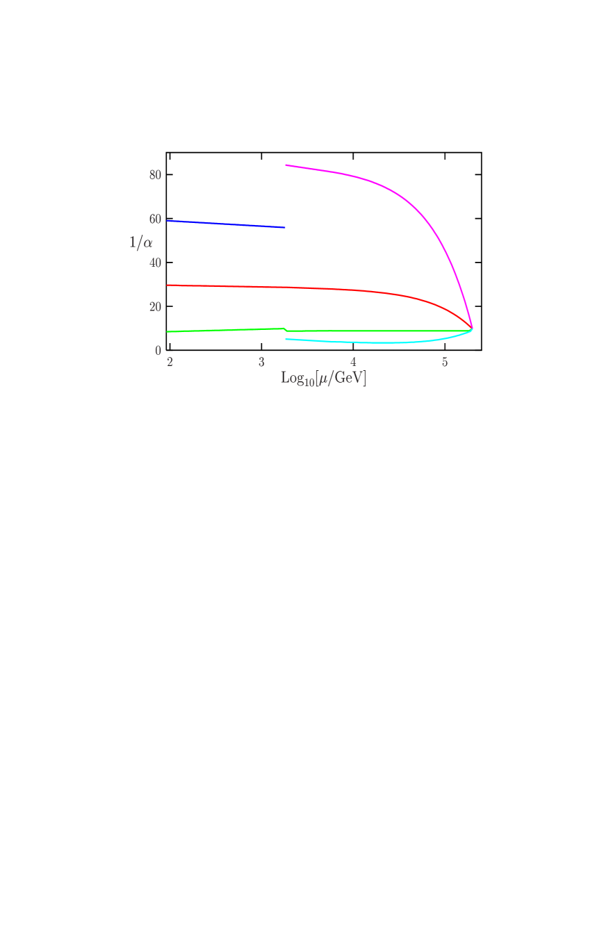
Figure 2: Low scale unification picture for model III-susy422 with $\alpha_{s}(M_{Z})\simeq 0.1184$ and $\eta=0$; $M_{I}=\mu_{0}\simeq 1.8$ TeV, $M_{G}\simeq 200$ TeV.

where $M_{D}$ is the mass of the zero mode of the doublet states $D^{\hskip 0.56905pt(1)}$, $\overline{D}^{\hskip 0.85358pt(2)}$, which arises from the 4D superpotential coupling $M_{D}D^{\hskip 0.56905pt(1)}\overline{D}^{\hskip 0.85358pt(2)}$. From (7.39) we see that for $S_{1}=S_{2}$ the contribution from KK states cancels out. Since $S_{1}$, $S_{2}$ differ slightly, the cancellation is partial and for a desirable value of $\alpha_{3}(M_{Z})$, appropriate contributions from the logarithmic terms are needed. Now, the contribution from KK states in (7.40) is always negative (there is no possible cancellation). Thus it is possible to get low scale unification in this scenario. The values of the mass scales, which give a successful picture of unification, are presented in Table 5. As one can see, for $M_{G}/\mu_{0}=110-107$ the couplings unify at the scale $M_{G}\simeq(200-400)$ TeV; the unified coupling constant $\alpha_{G}$($\simeq 0.1$) is perturbative. The picture of unification for case $M_{G}/\mu_{0}=110$ of Table 5 is presented in Fig. 2. Note, that in these cases the mass of the doublet pair $D^{\hskip 0.56905pt(1)}$, $\overline{D}^{\hskip 0.85358pt(2)}$ is $M_{D}\simeq(123-257)$ GeV. This makes the model testable in future collider experiments.

Table 5: Unification for the SUSY $G_{422}$ model III-susy422, with $\eta=0$. In all cases $\alpha_{G}\simeq 0.1$ is perturbative. Scales are measured in GeV units.

$$\begin{array}[]{|c|c|c|c|c|c|c|}\hline\cr M_{G}/\mu_{0}&(N,~{}N^{\prime})&\log_{10}[M_{I}]&\log_{10}[\mu_{0}]&\log_{10}[M_{G}]&\log_{10}[M_{G}/M_{D}]&\alpha_{3}(M_{Z})\\ \hline\cr\hline\cr 110&(54,~{}54)&3.26&3.26&5.30&3.21&0.1184\\ \hline\cr 108&(53,~{}53)&3.48&3.48&5.52&3.21&0.1185\\ \hline\cr 107&(52,~{}53)&3.6&3.6&5.62&3.21&0.1186\\ \hline\cr 106&(52,~{}52)&3.71&3.71&5.73&3.21&0.1186\\ \hline\cr\end{array}$$

7.2 $G_{422}\to G_{321}$ via $SU(3)\times SU(2)_{L}\times SU(2)_{R}\times U(1)^{\prime}$ compactification
breaking and related phenomenology

In this subsection, similar to 7.1, we will consider the breaking of $G_{422}$ by orbifold compactification down to $SU(3)\times SU(2)_{L}\times SU(2)_{R}\times U(1)^{\prime}\equiv G_{3221}$. The breaking of the latter to $G_{321}$ again will occur on the 4D level through the non-vanishing VEVs of certain fields.

The decomposition of $V(15_{c})$ ($\Sigma(15_{c})$) under $SU(3)_{c}\times U(1)^{\prime}$ is given in (7.1). The gauge group $SU(2)_{L}\times SU(2)_{R}$ is, in this case, not broken by the compactification.

The matter sector is the same as in (7.5) with copies (7.8) needed if chiral states are introduced in the bulk. The content of $F$, $F^{c}$ from the viewpoint of $G_{3221}$ is

$$F=q(3,~{}2,~{}1)_{1}+l(1,~{}2,~{}1)_{-3}~{},~{}~{}~{}F^{c}=q^{c}(\bar{3},~{}1,~{}2)_{-1}+l^{c}(1,~{}1,~{}2)_{3}~{},$$ (7.42)

where

$$q^{c}=(u^{c},~{}d^{c}),\quad l^{c}=(e^{c},~{}\nu^{c})~{}.$$ (7.43)

For the copies we have similar expressions.

To obtain one pair of MSSM Higgs doublets, it is enough in this case to have only one $N=2$ supermultiplet ${\bf\Phi}_{N=2}=(\Phi,~{}\overline{\Phi})$ (see (7.9)) with field content as in (7.10), (7.11).

For further $SU(2)_{R}\times U(1)^{\prime}$ breaking to $U(1)_{Y}$ we need the states (7.12) with components (7.13), (7.14) where now under $G_{3221}$ $H^{c}$ decomposes as

$$H^{c}=q^{c}_{H}(\bar{3},~{}1,~{}2)_{-1}+l^{c}_{H}(1,~{}1,~{}2)_{3}~{}$$ (7.44)

and similarly for $H^{\prime}$, $\overline{H}^{c}$, ${\overline{H}^{c}}^{\prime}$. The $Z_{2}\times Z_{2}^{\prime}$ parities and $U(1)^{\prime}$ charges of the appropriate fragments are given in Table 6. With these parity assignments, $G_{422}$ is broken to $G_{3221}$ and the zero mode matter and ’scalar’ superfields are $q$, $l^{\prime}$, $q^{c}$, ${l^{c}}^{\prime}$, $\Phi$, $l^{c}_{H}$, ${\overline{l}^{c}_{H}}^{\prime}$.

Table 6: $U(1)^{\prime}$ charges and $Z_{2}\times Z_{2}^{\prime}$ parities of the various fragments. All mirrors have opposite charges and parities.

$$\begin{array}[]{|c|c|c|}\hline\cr N=1~{}\textup{superfield}&\sqrt{24}\cdot Y_{U(1)^{\prime}}&Z_{2}\times Z_{2}^{\prime}\\ \hline\cr\hline\cr V_{c},~{}V_{L},~{}V_{s},~{}V_{R}&0&(+,~{}+)\\ \hline\cr\Sigma_{c},~{}\Sigma_{L},~{}\Sigma_{s},~{}\Sigma_{R}&0&(-,~{}-)\\ \hline\cr V_{t},~{}V_{\bar{t}}&4,-4&(-,~{}+)\\ \hline\cr\Sigma_{t},~{}\Sigma_{\bar{t}}&4,-4&(+,~{}-)\\ \hline\cr\hline\cr q~{},~{}q^{\prime}&1&(+,~{}+),~{}(-,~{}+)\\ \hline\cr l~{},~{}l^{\prime}&-3&(-,~{}+),~{}(+,~{}+)\\ \hline\cr q^{c}~{},~{}{q^{c}}^{\prime}&-1&(+,~{}+),~{}(-,~{}+)\\ \hline\cr l^{c}~{},~{}{l^{c}}^{\prime}&3&(-,~{}+),~{}(+,~{}+)\\ \hline\cr\hline\cr\Phi&0&(+,~{}+)\\ \hline\cr\hline\cr l^{c}_{H}~{},~{}{l^{c}_{H}}^{\prime}&3,-3&(+,~{}+)\\ \hline\cr q^{c}_{H}~{},~{}{q^{c}_{H}}^{\prime}&-1,1&(-,~{}+)\\ \hline\cr\end{array}$$

The $SU(2)_{R}\times U(1)^{\prime}\to U(1)_{Y}$ breaking occurs through $l^{c}_{H}$, ${\overline{l}^{c}_{H}}^{\prime}$ states, after their neutral scalar components $\nu^{c}_{H}$, ${\overline{\nu}^{c}_{H}}^{\prime}$ have developed non-zero VEV’s. As for the models considered above, here we also introduce a discrete ${\cal Z}$ symmetry. The combination ${\overline{l}^{c}_{H}}^{\prime}l^{c}_{H}$ transforms similarly to (4.4) and the relevant couplings will be (4.6)-(4.8) but with ${\cal S}$, $\overline{\cal S}$ replaced by $l^{c}_{H}$, ${\overline{l}^{c}_{H}}^{\prime}$. Thus, $\nu^{c}_{H}$ and ${\overline{\nu}^{c}_{H}}^{\prime}$ which are components of $l^{c}_{H}$ and ${\overline{l}^{c}_{H}}^{\prime}$ resp. will have non-vanishing VEV’s (7.16), (7.17). This provides the symmetry breaking down to $G_{321}$ at an intermediate mass scale between the SUSY scale $m$ and the unification scale $M$. As a first example suppose that $M\sim 10^{16}$GeV in which case $v\sim 10^{16}10^{-7/(n-1)}$GeV. With $n=7$ we get $v\stackrel{{\scriptstyle<}}{{{}_{\sim}}}M$, the value needed to have successful high scale unification in the I’-susy422 model (see below). On the other hand if the unification scale is as small as $M\sim 10^{6}$GeV, with $n=2$ we obtain $v\sim 10^{4}$GeV as needed in low scale unification scenarios.

With $\Phi$ transforming under ${\mathcal{Z}}$ as

$$\Phi\to e^{i\frac{\pi}{n}}\Phi~{},$$ (7.45)

the coupling responsible for the $\mu$-term generation is

$$W_{\mu}=M\left(\frac{{\overline{l}^{c}_{H}}^{\prime}l^{c}_{H}}{M^{2}}\right)^{n-1}\Phi^{2},$$ (7.46)

and we obtain the same $\mu$ term as in (7.19). The 4D Yukawa superpotential, responsible for generation of up-down quark and charged lepton masses, is

$$W_{Y}=qq^{c}\Phi+l^{\prime}{l^{c}}^{\prime}\Phi~{}.$$ (7.47)

From this coupling the Dirac type coupling for the neutrinos is also generated and $\hat{m}^{D}_{\nu}\sim\hat{m}_{e}$. There is therefore no additional suppression of the Dirac neutrino masses. For a low fundamental scale this turns out to be a problem. To overcome this difficulty we can introduce an additional singlet state ${\mathcal{N}}$. The relevant couplings are

$$\frac{1}{M}\left(\frac{{l^{c}_{H}}^{\prime}l^{c}_{H}}{M^{2}}\right)^{k}{\mathcal{N}}l^{c}_{H}\Phi l^{\prime}+{l^{c}_{H}}^{\prime}{l^{c}}^{\prime}{\mathcal{N}}.$$ (7.48)

Due to the last term in (7.48) the state ${\nu^{c}}^{\prime}$ decouples at the scale $\langle\nu^{c}_{H}\rangle\equiv M_{I}$ and the first term, which violates lepton number, is suppressed by appropriate powers of $M_{I}/M$. This can lead to a neutrino mass generation of the needed magnitude. It is not difficult to verify that together with the ${\nu^{c}}^{\prime}{\nu}^{\prime}h_{u}$ coupling, the operators in (7.48) give

$$m_{\nu}\sim\left(\frac{M_{I}}{M}\right)^{2k}\frac{\langle h_{u}^{0}\rangle^{2}}{M}~{}.$$ (7.49)

Note that we consider $M_{I}\ll M$ and therefore for $k>0$ one can obtain the needed suppression. For instance, with $k=1,2$, $M_{I}/M\sim 3\cdot 10^{-4}-10^{-2}$ and $M=(10^{6}-10^{9})$ GeV, one can have $m_{\nu}\sim 1$ eV.

7.2.1 Gauge coupling unification in 5D SUSY with $G_{422}\to G_{3221}$
intermediate breaking

Here we address the question of gauge coupling unification for $G_{422}$ with compactification breaking to $G_{3221}$.

Model I’-susy422

The field content of this scenario is minimal: $N=2$ gauge supermultiplets, scalar superfields, and $\eta$ generation of matter in the bulk. All these states, their $U(1)^{\prime}$ charges, and $Z_{2}\times Z_{2}^{\prime}$ parities are presented in Table 6. The corresponding $b^{M_{I}}$, $\gamma$, and $\delta$ factors are

$$(b_{U(1)^{\prime}},~{}b_{SU(2)_{R}},~{}b_{2},~{}b_{3})^{M_{I}}=\left(\frac{15}{2},~{}2,~{}1,-3\right),$$ (7.50)

$$(\gamma_{U(1)^{\prime}},~{}\gamma_{SU(2)_{R}},~{}\gamma_{2},~{}\gamma_{3})=\left(3,~{}0,-2,-6\right)+4\eta\left(1,~{}1,~{}1,~{}1\right),$$

$$(\delta_{U(1)^{\prime}},~{}\delta_{SU(2)_{R}},~{}\delta_{2},~{}\delta_{3})=\left(-7,~{}6,~{}0,~{}2\right)+4\eta\left(1,~{}1,~{}1,~{}1\right).$$ (7.51)

On the scale $M_{I}$ we have matching conditions (3.3), (3.4), where $G_{1}=SU(2)_{R}$, $G_{2}=U(1)^{\prime}$ and $\tan\theta=\sqrt{\frac{3}{2}}$. Taking all this into account, from (3.14)-(3.16) we obtain

$$\alpha_{3}^{-1}=\frac{12}{7}\alpha_{2}^{-1}-\frac{5}{7}\alpha_{1}^{-1}-\frac{6}{7\pi}\ln{\frac{M_{G}}{M_{I}}}-\frac{3}{7\pi}(2S_{1}-3S_{2}),$$ (7.52)

$$\ln{\frac{M_{I}}{M_{Z}}}=\frac{5\pi}{14}(\alpha_{1}^{-1}-\alpha_{2}^{-1})-\frac{4}{7}\ln{\frac{M_{G}}{M_{I}}}-\frac{1}{7}(4S_{1}+S_{2}),$$ (7.53)

$$\alpha_{G}^{-1}=\alpha_{2}^{-1}-\frac{1}{2\pi}\ln{\frac{M_{G}}{M_{Z}}}+\frac{1-2\eta}{\pi}S_{1}-\frac{2\eta}{\pi}S_{2}.$$ (7.54)

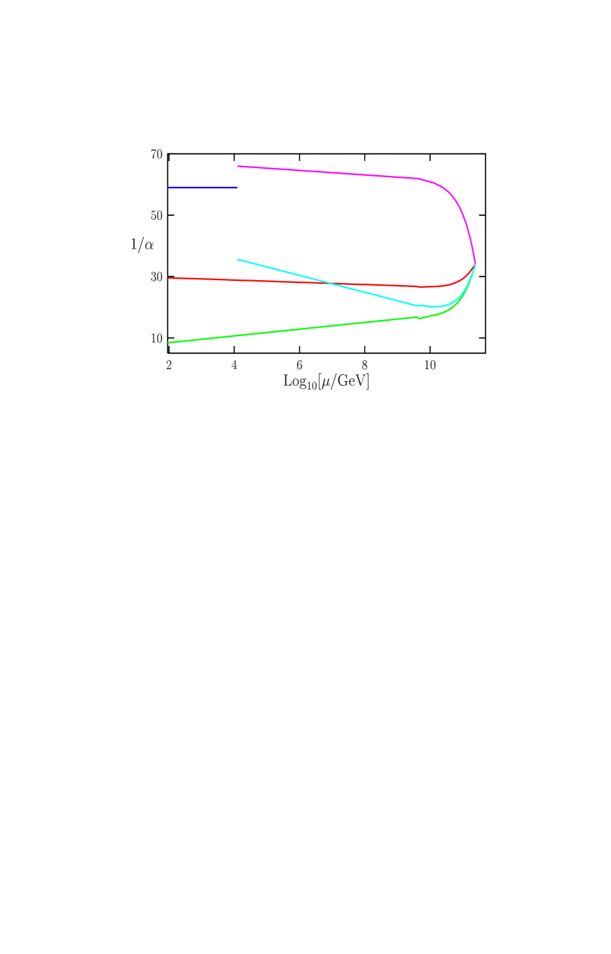
Figure 3: Unification picture for Model I’-susy422 with $\alpha_{s}(M_{Z})\simeq 0.119$ and $\eta=0$; $M_{I}\simeq 12.6$ TeV, $\mu_{0}\simeq 4.4\cdot 10^{9}$ GeV, $M_{G}\simeq 2.5\cdot 10^{11}$ GeV.

In Table 7 we present several solutions of the above equations. The experimental lower bound $M_{I}\stackrel{{\scriptstyle>}}{{{}_{\sim}}}10^{4}$GeV for the $SU(2)_{R}$ symmetry breaking scale [9], [54] puts a bound also on the unification scale $M_{G}\stackrel{{\scriptstyle>}}{{{}_{\sim}}}10^{11}$GeV. The picture of unification for the case in the last row of Table 7 is presented in Fig. 3.

Table 7: Unification in the model I’-susy422, with $\eta=0$. Mass scales are measured in GeV units and $\alpha_{3}=0.119$. In all cases $\alpha_{G}\simeq 0.03$ is perturbative.

$$\begin{array}[]{|c|c|c|c|c|c|}\hline\cr M_{G}/\mu_{0}&(N,~{}N^{\prime})&\log_{10}{[M_{I}]}&\log_{10}{[\mu_{0}]}&\log_{10}{[M_{G}]}\\ \hline\cr\hline\cr 50&(24,~{}24)&5.40&10.32&12.02\\ \hline\cr 51&(24,~{}25)&5.18&10.20&11.91\\ \hline\cr 55&(26,~{}27)&4.31&9.75&11.49\\ \hline\cr 56&(27,~{}27)&4.10&9.64&11.39\\ \hline\cr\end{array}$$

Model II’-susy422: low scale unification

In order to have low scale unification, as for the model III-susy422, we introduce two ${\bf 6}_{N=2}^{(i)}$ plets of $SU(4)_{c}$ (i=1, 2) with decomposition (7.24), and two ${\bf 2}_{N}=2^{(j)}=(D,~{}\overline{D})^{(j)}$ of $SU(2)_{L}$ ($j=1,2$). In addition we introduce one bi-doublet ${\bf\Phi^{\prime}}_{N=2}$ state of (7.9). We will take $Z_{2}\times Z_{2}^{\prime}$ parities (7.25) and (7.37) for fragments from ${\bf 6}_{N=2}^{(i)}$ and ${\bf 2}_{N=2}^{(j)}$, resp., while for the fragments of ${\bf\Phi^{\prime}}_{N=2}$ we take the parities $\Phi^{\prime}\sim(-,+)$, $\bar{\Phi}^{\prime}\sim(+,-)$. The contributions of these states to the $b$, $\gamma$, and $\delta$ factors are

$$(b_{U(1)^{\prime}},~{}b_{SU(2)_{R}},~{}b_{2},~{}b_{3})^{T}=\left(1,~{}0,~{}0,~{}1\right),$$ (7.55)

$$(b_{U(1)^{\prime}},~{}b_{SU(2)_{R}},~{}b_{2},~{}b_{3})^{D}=\left(0,~{}0,~{}1,~{}0\right),$$ (7.56)

$$({\bf\Delta_{6}}+{\bf\Delta_{2}})(\gamma_{U(1)^{\prime}},~{}\gamma_{SU(2)_{R}},~{}\gamma_{2},~{}\gamma_{3})=\left(2,~{}0,~{}0,~{}2\right)+\left(0,~{}0,~{}2,~{}0\right),$$

$$({\bf\Delta_{6}}+{\bf\Delta_{\Phi^{\prime}}})(\delta_{U(1)^{\prime}},~{}\delta_{SU(2)_{R}},~{}\delta_{2},~{}\delta_{3})=\left(2,~{}0,~{}0,~{}2\right)+\left(0,~{}2,~{}2,~{}0\right).$$ (7.57)

With these changes we obtain

$$\alpha_{3}^{-1}=\frac{12}{7}\alpha_{2}^{-1}-\frac{5}{7}\alpha_{1}^{-1}-\frac{6}{7\pi}\ln{\frac{M_{G}}{M_{I}}}+\frac{9}{14\pi}\ln{\frac{M_{G}}{M_{T}}}-\frac{6}{7\pi}\ln{\frac{M_{G}}{M_{D}}}-\frac{9}{7\pi}\left(S_{1}-S_{2}\right),$$ (7.58)

$$\ln{\frac{M_{I}}{M_{Z}}}=\frac{5\pi}{14}(\alpha_{1}^{-1}-\alpha_{2}^{-1})-\frac{4}{7}\ln{\frac{M_{G}}{M_{I}}}-\frac{1}{14}\ln{\frac{M_{G}}{M_{T}}}+\frac{5}{28}\ln{\frac{M_{G}}{M_{D}}}-\frac{1}{14}\left(5\,S_{1}+2\,S_{2}\right),$$ (7.59)

$$\alpha_{G}^{-1}=\alpha_{2}^{-1}-\frac{1}{2\pi}\ln{\frac{M_{G}}{M_{Z}}}-\frac{1}{2\pi}\ln{\frac{M_{G}}{M_{D}}}-\frac{2\eta}{\pi}S_{1}-\frac{1+2\eta}{\pi}S_{2}.$$ (7.60)

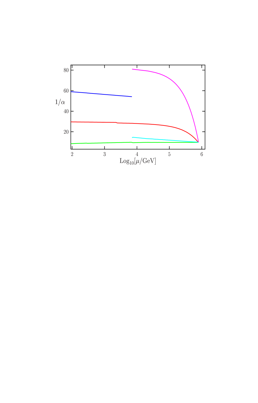
Figure 4: Low scale unification picture for Model II’-susy422 with $\alpha_{s}(M_{Z})\simeq 0.119$ and $\eta=0$; $M_{I}\simeq 7.1$ TeV, $\mu_{0}\simeq 7.2$ TeV, $M_{G}\simeq 794$ TeV.

In (7.58) the last term vanishes in the $S_{1}=S_{2}$ limit, while the last term of (7.59) is negative. This shows that low scale unification is possible. In Table 8 we present several cases of successful unification in this scenario. With the experimental bound $M_{I}\stackrel{{\scriptstyle>}}{{{}_{\sim}}}10^{4}$GeV we have $M_{G}\stackrel{{\scriptstyle>}}{{{}_{\sim}}}10^{6}$GeV. The picture of unification for the $M_{G}/\mu_{0}=110$ case of Table 8 is presented in Fig. 4.

Table 8: Unification in the model II’-susy422, with $\eta=0$. Mass scales are measured in GeV units and $\alpha_{3}=0.119$. In all cases $\alpha_{G}\simeq 0.1$ is perturbative.

$$\begin{array}[]{|c|c|c|c|c|c|c|c|}\hline\cr M_{G}/\mu_{0}&(N,~{}N^{\prime})&\log_{10}{[M_{G}/M_{T}]}&\log_{10}{[M_{G}/M_{D}]}&\log_{10}{[M_{I}]}&\log_{10}{[\mu_{0}]}&\log_{10}{[M_{G}]}\\ \hline\cr\hline\cr 110&(54,~{}54)&3.44&2.52&3.85&3.86&5.90\\ \hline\cr 109&(53,~{}54)&3.62&2.65&3.97&3.98&6.00\\ \hline\cr 108&(53,~{}53)&3.80&2.80&4.10&4.10&6.15\\ \hline\cr 107&(52,~{}53)&3.78&2.78&4.21&4.21&6.23\\ \hline\cr 90&(44,~{}44)&5.26&1.96&4.71&6.67&8.63\\ \hline\cr 89&(43,~{}44)&5.42&1.95&4.73&6.82&8.77\\ \hline\cr 80&(39,~{}39)&7.90&1.90&4.45&8.46&10.36\\ \hline\cr\end{array}$$

Model III’-susy422: low scale unification

A different model which also gives low scale unification is a scenario extended with ${\bf\Phi^{\prime}}_{N=2}$ and four ${\bf R}^{r}_{N=2}=(R,~{}\overline{R})^{(r)}$ ($r=1,\cdots,4$), where $R$ is a doublet of $SU(2)_{R}$. With $Z_{2}\times Z_{2}^{\prime}$ parities

$$R^{(r)}\sim(+,~{}+)~{},~{}~{}~{}\overline{R}^{(r)}\sim(-,~{}-)~{},$$ (7.61)

their contributions to the $b$-factors (above the common mass $M_{R}$) and $\gamma$, $\delta$ factors are

$$(b_{U(1)^{\prime}},~{}b_{SU(2)_{R}},~{}b_{2},~{}b_{3})^{M_{R}}=\left(0,~{}2,~{}0,~{}0\right),$$ (7.62)

$${\bf\Delta_{R}}(\gamma_{U(1)^{\prime}},~{}\gamma_{SU(2)_{R}},~{}\gamma_{2},~{}\gamma_{3})=(0,~{}4,~{}0,~{}0).$$ (7.63)

RGEs in this case are

$$\alpha_{3}^{-1}=\frac{12}{7}\alpha_{2}^{-1}-\frac{5}{7}\alpha_{1}^{-1}-\frac{6}{7\pi}\ln{\frac{M_{G}}{M_{I}}}+\frac{3}{7\pi}\ln{\frac{M_{G}}{M_{R}}},$$ (7.64)

$$\ln{\frac{M_{I}}{M_{Z}}}=\frac{5\pi}{14}(\alpha_{1}^{-1}-\alpha_{2}^{-1})-\frac{4}{7}\ln{\frac{M_{G}}{M_{I}}}-\frac{3}{14}\ln{\frac{M_{G}}{M_{R}}}-S_{1},$$ (7.65)

$$\alpha_{G}^{-1}=\alpha_{2}^{-1}-\frac{1}{2\pi}\ln{\frac{M_{G}}{M_{Z}}}+\frac{1-2\eta}{\pi}S_{1}-\frac{1+2\eta}{\pi}S_{2}.$$ (7.66)

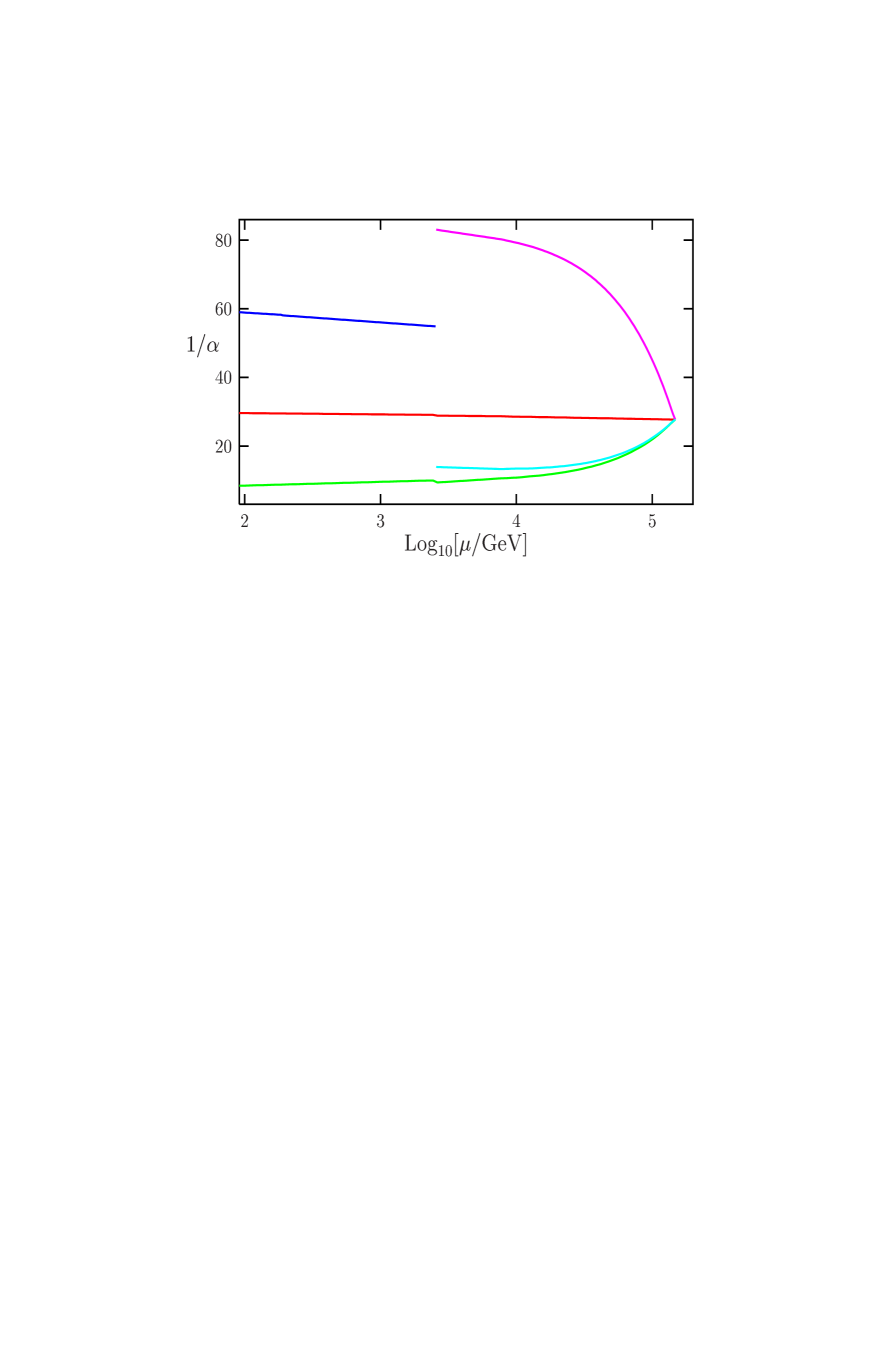
Figure 5: Low scale unification picture for model III’-susy422 with $\alpha_{s}(M_{Z})\simeq 0.119$ and $\eta=0$; $M_{I}=\mu_{0}\simeq 2.6$ TeV, $M_{G}\simeq 148$ TeV.

From the above equations we see that this scenario also allows low scale unification. In Table 9 we present mass scales giving successful unification. In this case the experimental bound $M_{I}\stackrel{{\scriptstyle>}}{{{}_{\sim}}}10^{4}$ GeV gives $M_{G}\stackrel{{\scriptstyle>}}{{{}_{\sim}}}10^{5.8}$GeV. The picture of unification for the $M_{G}/\mu_{0}=57$ case of Table 9 is presented in Fig. 5.

Table 9: Unification in the model III’-susy422, with $\eta=0$. Mass scales are measured in GeV units and $\alpha_{3}=0.119$. In all cases $\alpha_{G}\simeq 0.04$ is perturbative.

$$\begin{array}[]{|c|c|c|c|c|c|c|}\hline\cr M_{G}/\mu_{0}&(N,~{}N^{\prime})&\log_{10}{[M_{G}/M_{R}]}&\log_{10}{[M_{I}]}&\log_{10}{[\mu_{0}]}&\log_{10}{[M_{G}]}\\ \hline\cr\hline\cr 57&(27,~{}28)&2.89&3.41&3.41&5.17\\ \hline\cr 55&(26,~{}27)&2.85&3.85&3.85&5.59\\ \hline\cr 54&(26,~{}26)&2.84&4.08&4.08&5.81\\ \hline\cr 53&(25,~{}26)&2.82&4.30&4.30&6.02\\ \hline\cr 37&(17,~{}18)&7.11&5.55&7.85&9.42\\ \hline\cr 36&(17,~{}17)&7.29&5.67&8.07&9.63\\ \hline\cr 18&(8,~{}8)&11.08&7.54&12.14&13.39\\ \hline\cr 17&(7,~{}8)&11.24&7.66&12.36&13.59\\ \hline\cr\end{array}$$

8 5D flipped $SU(5)\times U(1)$ model
on $S^{(1)}/Z_{2}\times Z_{2}^{\prime}$ orbifold

Finally we consider flipped $SU(5)\times U(1)\equiv G_{51}$ GUT in 5D. The decomposition of $SU(5)$’s adjoint $V(24)$ in terms of $SU(3)_{c}\times SU(2)_{L}\times U(1)^{\prime}$ reads

$$V(24)=V_{c}(8,1)_{0}+V_{SU(2)_{L}}(1,3)_{0}+V_{s}(1,1)_{0}+V_{X}(3,\bar{2})_{5}+V_{Y}(\bar{3},2)_{-5}~{},$$ (8.1)

where subscripts denote $U(1)^{\prime}$ charges in $1/\sqrt{60}$ units. Since the $U(1)^{\prime}$ comes from $SU(5)$, it has the usual $1/\sqrt{60}$ normalization. $V_{s}$ in (8.1) corresponds to the $U(1)^{\prime}$ gauge superfield. The decomposition of $\Sigma(24)$ has an identical form.

Matter  sector

The matter sector contains $\eta$ generations of $N=2$ supermultiplets

$${\bf X}_{N=2}=({\cal X},~{}\overline{\cal X})~{},~{}~{}~{}~{}{\bf V}_{N=2}=({\cal V},~{}\overline{\cal V})~{},~{}~{}~{}~{}{\bf I}_{N=2}=({\cal I},~{}\overline{\cal I})~{},$$ (8.2)

where

$${\cal X}={\bf 10}_{-1}=(\nu^{c},~{}q,~{}d^{c})_{-1}~{},~{}~{}{\cal V}=\bf{\bar{5}}_{3}=(l,~{}u^{c})_{3}~{},~{}~{}{\cal I}={\bf 1}_{-5}=e^{c}_{-5}~{}$$ (8.3)

are the usual chiral multiplets of flipped $SU(5)\times U(1)$ GUT, and $\overline{\cal X}$, $\overline{\cal V}$, $\overline{\cal I}$ in (8.2) are their mirrors. Subscripts in (8.3) denote $U(1)$ charges, defined up to some normalization factor. Assuming that $G_{51}$ comes from $SO(10)$, the normalization factor will be $1/\sqrt{40}$. Therefore, in $SO(10)$ normalization

$$Y_{U(1)}[{\cal X}]=-\frac{1}{\sqrt{40}}~{},~{}~{}~{}Y_{U(1)}[{\cal V}]=\frac{3}{\sqrt{40}}~{},~{}~{}~{}Y_{U(1)}[{\cal I}]=-\frac{5}{\sqrt{40}}~{},~{}$$ (8.4)

In fact, the $SO(10)$ spinor ${\bf 16}$ in terms of $G_{51}$ reads

$${\bf 16}_{SO(10)}={\bf 10}_{-1}+{\bf\bar{5}}_{3}+{\bf 1}_{-5}~{}.$$ (8.5)

We also introduce $\eta$ copies ${\bf X^{\prime}}_{N=2}$, ${\bf V^{\prime}}_{N=2}$, ${\bf I^{\prime}}_{N=2}$. $3-\eta$ generations are introduced at the brane.

Scalar sector

To have MSSM doublets we introduce the following set of supermultiplets:

$${\bf h}_{N=2}=\left(h(5_{2}),~{}\overline{h}(\bar{5}_{-2})\right)~{},~{}~{}~{}~{}{\bf h}_{N=2}^{\prime}=\left(h^{\prime}(5_{-2}),~{}\bar{h}^{\prime}(\bar{5}_{-2})\right)~{},$$ (8.6)

where subscripts denote $U(1)$ charges in $1/\sqrt{40}$ units. In (8.6) one has

$$h(5_{2})=(h_{d},~{}\overline{d}^{c}_{h})_{2}~{},~{}~{}~{}~{}~{}\overline{h}(\bar{5}_{-2})=(h_{u},~{}d^{c}_{\bar{h}})_{-2}~{},$$ (8.7)

and the same for states with primes.

For reducing the rank of the group via Higgs breaking we need additional states. Thus we introduce

$${\bf H}_{N=2}=\left(H,~{}\overline{H}\right)~{},~{}~{}~{}~{}~{}{\bf H}_{N=2}^{\prime}=\left(H^{\prime},~{}\overline{H}\hskip 0.85355pt^{\prime}\right)~{},$$ (8.8)

where

$$H=10_{-1}^{H}=\left(\nu^{c}_{H},~{}d^{c}_{H},~{}q^{~{}}_{H}\right)_{-1}~{},~{}~{}~{}\overline{H}=\overline{10}^{H}_{1}=\left(\overline{\nu}^{c}_{H},~{}\overline{d}^{c}_{H},~{}\overline{q}^{~{}}_{H}\right)_{1}~{},$$ (8.9)

and similarly for $H^{\prime}$ and $\overline{H}\hskip 0.85355pt^{\prime}$.

8.1 $G_{51}\to G_{321}$ breaking and related phenomenological questions

The first stage of breakdown of the $G_{51}$ gauge group again occurs through orbifolding: prescribing to various fragments of $G_{51}$ multiplets certain $Z_{2}\times Z_{2}^{\prime}$ parities some states are projected out, and at a fixed point we remain with a reduced gauge group. The transformation properties of the fragments of 5D SUSY $G_{51}$ are given in Table 10.

Table 10: $U(1)$, $U(1)^{\prime}$ charges and $Z_{2}\times Z_{2}^{\prime}$ parities of various fragments in 5D SUSY $G_{51}$ scenario. All mirrors, of matter and scalars, have opposite charges and parities.

$$\begin{array}[]{|c|c|c|c|}\hline\cr N=1~{}{\rm superfield}&\sqrt{40}\cdot Y_{U(1)}&\sqrt{60}\cdot Y_{U(1)^{\prime}}&Z_{2}\times Z_{2}^{\prime}\\ \hline\cr\hline\cr V_{c},~{}V_{SU(2)_{L}},~{}V_{U(1)},~{}V_{s}&0&0&(+,~{}+)\\ \hline\cr\Sigma_{c},~{}\Sigma_{SU(2)_{L}},~{}\Sigma_{U(1)},~{}\Sigma_{s}&0&0&(-,~{}-)\\ \hline\cr V_{X}~{},~{}V_{Y}&0&5,~{}-5&(-,~{}+)\\ \hline\cr\Sigma_{X}~{},~{}\Sigma_{Y}&0&5,~{}-5&(+,~{}-)\\ \hline\cr\hline\cr q~{}~{},~{}~{}q\hskip 1.70717pt^{\prime}&-1&-1&(+,~{}+),~{}(-,~{}+)\\ \hline\cr l~{}~{},~{}~{}l\hskip 1.70717pt^{\prime}&3&3&(+,~{}+),~{}(-,~{}+)\\ \hline\cr u^{c}~{}~{},~{}~{}{u^{c}}^{\prime}&3&-2&(-,~{}+),~{}(+,~{}+)\\ \hline\cr d^{c}~{}~{},~{}~{}{d^{c}}^{\prime}&-1&4&(-,~{}+),~{}(+,~{}+)\\ \hline\cr\nu^{c}~{}~{},~{}~{}{\nu^{c}}^{\prime}&-1&-6&(-,~{}+),~{}(+,~{}+)\\ \hline\cr e^{c}~{}~{},~{}~{}{e^{c}}^{\prime}&-5&0&(+,~{}+),~{}(-,~{}+)\\ \hline\cr\hline\cr h_{u}~{}~{},~{}~{}{h_{d}}^{\prime}&-2,~{}2&3,~{}-3&(+,~{}+)\\ \hline\cr{d^{c}}_{\bar{h}}~{}~{},~{}~{}{\bar{d}^{c^{\prime}}_{h}}&-2,~{}2&-2,~{}2&(-,~{}+)\\ \hline\cr\nu^{c}_{H}~{}~{},~{}~{}{\overline{\nu}^{c}_{H}}^{\prime}&-1,~{}1&-6,~{}6&(+,~{}+)\\ \hline\cr d^{c}_{H}~{}~{},~{}~{}{\overline{d}^{c}_{H}}^{\prime}&-1,~{}1&4,~{}-4&(+,~{}+)\\ \hline\cr q^{~{}}_{H}~{}~{},~{}~{}{\overline{q}^{~{}}_{H}}^{\prime}&-1,~{}1&-1,~{}1&(-,~{}+)\\ \hline\cr\end{array}$$

One can easily see that at the $y=0$ fixed point we have a $SU(3)_{c}\times SU(2)_{L}\times U(1)\times U(1)^{\prime}\equiv{G^{\prime}}_{3211}$ gauge group. At this fixed point together with three generations of quark-lepton and right handed neutrino superfields $q$, ${u^{c}}^{\prime}$, ${d^{c}}^{\prime}$, $l$, $e^{c}$, ${\nu^{c}}^{\prime}$ and an MSSM pair of Higgs doublets $h_{u}$, ${h_{d}}^{\prime}$, we also have the states $d^{c}_{H}$, ${\overline{d}^{c}_{H}}^{\prime}$, $\nu^{c}_{H}$, ${\overline{\nu}^{c}_{H}}^{\prime}$. The latter two states are responsible for an $U(1)\times U(1)^{\prime}$ breaking down to $U(1)_{Y}$. If they develop VEVs on the scale $M_{I}$ the second stage of symmetry breaking occurs and we have the unbroken $U(1)_{Y}$ generator

$$Y=\frac{2\sqrt{6}}{5}Y_{U(1)}-\frac{1}{5}Y_{U(1)^{\prime}}~{},$$ (8.10)

where $Y_{U(1)^{\prime}}$ and $Y_{U(1)}$ charges of the states are given in Table 10. [For $Y_{U(1)}$ again we have used $SO(10)$ normalization (8.4), since flipped $SU(5)\times U(1)$ is one of its maximal subgroups [35], [36]].

The generation of $\langle\nu^{c}_{H}\rangle$, $\langle{\overline{\nu}^{c}_{H}}^{\prime}\rangle$ VEVs can happen in the same way as for the $SU(4)_{c}\times SU(2)_{L}\times SU(2)_{R}$ scenario presented in sect. 7.1. Introducing a discrete ${\cal Z}$ symmetry and a transformation for ${\overline{\nu}^{c}_{H}}^{\prime}\nu^{c}_{H}$ as in (4.4), the relevant superpotential, soft SUSY breaking, and all the potential couplings will have the form of (4.6), (4.7), (4.8) resp. if the states ${\cal S}$, $\overline{\cal S}$ are replaced by $\nu^{c}_{H}$, ${\overline{\nu}^{c}_{H}}^{\prime}$. From all this one can ensure non zero VEV solutions (7.16), (7.17). By a proper choice of $n$ one can obtain a gap between the mass scales $v\equiv M_{I}$ and $M$. Also $\mu$ term generation can happen similarly. With transformation (4.3) for the $h_{u}{h_{d}}^{\prime}$ combination and coupling (7.18) the $\mu$ term (7.19) is derived.

Also for the SUSY $G_{51}$ model we use a ${\cal Z}$ symmetry to obtain a realistic phenomenology. The Lagrangian (2.3), (2.4) with $Z_{2}\times Z_{2}^{\prime}$ orbifold parities should be invariant under this ${\cal Z}$; therefore the fragments of matter and scalar superfields from the same $SU(5)\times U(1)$ multiplets should have identical ${\cal Z}$ phases, while the phases of mirrors must be opposite. Together with quark-lepton superfields and right handed neutrinos at the $y=0$ fixed point we have zero mode $\nu^{c}_{H}$, ${\overline{\nu}^{c}_{H}}^{\prime}$, $d^{c}_{H}$, ${\overline{d}^{c}_{H}}^{\prime}$ states. With couplings (4.6) (with $\overline{\cal S}{\cal S}$ replaced by ${\overline{\nu}^{c}_{H}}^{\prime}{\nu}^{c}_{H}$), (7.18) we thus have

$$\alpha(\nu^{c}_{H})+\alpha({\overline{\nu}^{c}_{H}}^{\prime})=\alpha({h_{d}}^{\prime})+\alpha(h_{u})=\frac{2\pi}{n}~{},$$ (8.11)

and

$$\alpha({\nu^{c}}^{\prime})=\alpha({d^{c}}^{\prime})~{},~{}~{}~{}\alpha(\nu^{c}_{H})=\alpha(d^{c}_{H})~{},~{}~{}~{}\alpha({\overline{\nu}^{c}_{H}}^{\prime})=\alpha({\overline{d}^{c}_{H}}^{\prime})~{}.$$ (8.12)

Therefore, at this stage together with the phases of $q$, $u^{c}$, $l$, $e^{c}$, we have 8 independent phases. Writing Yukawa couplings which generate masses for up-down quarks and charged leptons

$$W_{Y}=q{u^{c}}^{\prime}h_{u}+q{d^{c}}^{\prime}{h_{d}}^{\prime}+le^{c}{h_{d}}^{\prime}~{},$$ (8.13)

we will remain with 4 independent phases. It is possible to fix two of them from the neutrino sector, writing Dirac and Majorana type couplings. For the question of the mass scales needed for successful unification the couplings of type (7.21) are irrelevant, while terms ${\nu^{c}}^{\prime}lh_{u}+\frac{1}{M}({\overline{\nu}^{c}_{H}}^{\prime}{\nu^{c}}^{\prime})^{2}$ give $m_{\nu}\sim\frac{h_{u}^{2}}{M_{I}^{2}}M$. The latter leads to the reasonable value $m_{\nu}\sim 1$ eV for $M_{G}/\mu_{0}=1$ in Table 11. However, through these couplings the phases of appropriate states are selected in such a way, that some unacceptably large matter parity (lepton number) and baryon number violating couplings are allowed. To avoid this, we will modify to a model, which gives a value for the neutrino mass accommodating atmospheric data and does not lead to any unacceptable process. Including a matter parity violating (4.11) type coupling

$$\left(\frac{{\overline{\nu}^{c}_{H}}^{\prime}\nu^{c}_{H}}{M^{2}}\right)^{n-1}\nu^{c}_{H}lh_{u}~{},$$ (8.14)

similar to the treatment in the MSSM and $SU(5)$ cases, one obtains an operator $\mu_{l}lh_{u}$ with $\mu_{l}\sim\frac{M_{I}}{M}m$ inducing a neutrino mass (4.13), where in this case $\sin\xi\sim\frac{M_{I}}{M}$ (still without assuming any alignment between superpotential and soft SUSY breaking couplings). For a suppressed neutrino mass we need $M_{I}/M\leq 3\cdot 10^{-6}$. This case indeed is realized with successful unification [see case $M_{G}/\mu=5$ in Table 11]: for $M_{I}\simeq 6\cdot 10^{10}$ GeV and $M=M_{G}\simeq 2\cdot 10^{16}$ GeV, three gauge couplings are unified and we have $m_{\nu}\stackrel{{\scriptstyle<}}{{{}_{\sim}}}1$ eV.

Couplings (8.13), (8.14) and conditions (8.11), (8.12) determine the phases

$$\alpha({h_{d}}^{\prime})=\alpha-\alpha(h_{u})~{},~{}~{}\alpha({u^{c}}^{\prime})=-\alpha(q)-\alpha(h_{u})~{},~{}~{}\alpha(e^{c})=-\alpha(l)+\alpha(h_{u})-\alpha~{},$$

$$\alpha({\nu^{c}}^{\prime})=\alpha({d^{c}}^{\prime})=-\alpha(q)+\alpha(h_{u})-\alpha~{},~{}~{}\alpha(\nu^{c}_{H})=\alpha(d^{c}_{H})=\alpha-\alpha(l)-\alpha(h_{u})~{},$$

$$\alpha({\overline{\nu}^{c}_{H}}^{\prime})=\alpha({\overline{d}^{c}_{H}}^{\prime})=\alpha(l)+\alpha(h_{u})~{},~{}~{}~{}\alpha=\frac{2\pi}{n}~{},$$ (8.15)

but $\alpha(q)$, $\alpha(l)$, $\alpha(h_{u})$ are still free. With eqs. (8.15) the lepton number violating operators

$$\frac{\nu^{c}_{H}}{M}q{d^{c}}^{\prime}l~{},~{}~{}~{}~{}~{}\frac{\nu^{c}_{H}}{M}e^{c}ll~{},$$ (8.16)

are allowed, and for $M_{I}/M\sim 3\cdot 10^{-6}$ they lead to a radiative neutrino mass $m_{\nu}^{\prime}\sim 10^{-5}$ eV [see eq. (4.17), (4.16)], with the relevant scale for the solar neutrino anomaly.

Chosing $\alpha(q)$, $\alpha(l)$ and $\alpha(h_{u})$ as

$$\alpha(q)=\alpha(l)=\alpha/3,~{}~{}~{}~{}~{}\alpha(h_{u})=\alpha~{},$$ (8.17)

the discrete ${\cal Z}$ symmetry will be $Z_{3n}$. With assignment (8.15), (8.17) the coupling $\nu^{c}_{H}qld^{c}_{H}$ is allowed. However, the coupling ${\overline{\nu}^{c}_{H}}^{\prime}qq{\overline{d}^{c}_{H}}^{\prime}$ is forbidden and therefore the $d=5$ operator $qqql$ does not emerge. One can verify easily that all other matter parity and baryon number violating operators are absent in this setting. The coupling $\nu^{c}_{H}qld^{c}_{H}$ would induce decays of a light triplet $d^{c}_{H}$ (mass $\sim$ few TeV) $d^{c}_{H}\to ql$ with leptoquark signature, observable in future collider experiments [53].

Concluding this subsection we note that in order to give masses to the states ${\nu^{c}}^{\prime}$ one can introduce ${\cal N}$ singlet states with $Z_{3n}$ phase $\alpha({\cal N})=-\alpha$. Through couplings ${\overline{\nu}^{c}_{H}}^{\prime}{\nu^{c}}^{\prime}{\cal N}$ right handed states would decouple at the scale $M_{I}$.

8.2 Gauge coupling unification in 5D SUSY $G_{51}$

Below $M_{I}$ we have the MSSM field content with the b-factors (4.21), plus states $d^{c}_{H}$, ${\overline{d}^{c}_{H}}^{\prime}$ with mass $M_{d^{c}_{H}}$ in the TeV range and b-factors as in (7.27). Above the $M_{I}$ scale we obtain

$$\left(b_{U(1)},~{}b_{U(1)^{\prime}},~{}b_{2},~{}b_{3}\right)^{M_{I}}=\left(\frac{33}{5},~{}\frac{47}{5},~{}1,~{}-2\right)~{},$$ (8.18)

and for the $\gamma$ and $\delta$ factors

$$\left(\gamma^{~{}}_{U(1)},~{}\gamma^{~{}}_{U(1)^{\prime}},~{}\gamma_{2},~{}\gamma_{3}\right)=\left(\frac{6}{5},~{}\frac{34}{5},~{}-2,~{}-4\right)+4\eta(1,~{}1,~{}1,~{}1)~{},$$

$$\left(\delta_{U(1)},~{}\delta_{U(1)^{\prime}},~{}\delta_{2},~{}\delta_{3}\right)=\left(\frac{9}{5},~{}-\frac{44}{5},~{}0,~{}2\right)+4\eta(1,~{}1,~{}1,~{}1)~{},$$ (8.19)

if $\eta$ families have KK excitations.

According to (8.10), we get $\tan\theta=2\sqrt{6}$ for the $\tan\theta$ in (3.3) if $G_{1}=U(1)$ and $G_{2}=U(1)^{\prime}$. Taking into account this and also (3.2)-(3.16) one obtains

$$\alpha_{3}^{-1}=\frac{12}{7}\alpha_{2}^{-1}-\frac{5}{7}\alpha_{1}^{-1}+\frac{27}{50\pi}\ln\frac{M_{G}}{M_{I}}+\frac{9}{14\pi}\ln\frac{M_{I}}{M_{d^{c}_{H}}}+\frac{39}{175\pi}S_{1}+\frac{261}{175\pi}S_{2}~{},$$ (8.20)

$$\ln\frac{M_{I}}{M_{Z}}=\frac{5\pi}{14}(\alpha_{1}^{-1}-\alpha_{2}^{-1})-\frac{51}{50}\ln\frac{M_{G}}{M_{I}}-\frac{1}{14}\ln\frac{M_{I}}{M_{d^{c}_{H}}}-\frac{107}{175}S_{1}-\frac{43}{175}S_{2}~{},$$ (8.21)

$$\alpha_{G}^{-1}=\alpha_{2}^{-1}-\frac{1}{2\pi}\ln\frac{M_{G}}{M_{Z}}+\frac{1-2\eta}{\pi}S_{1}-\frac{2\eta}{\pi}S_{2}~{}.$$ (8.22)

The last four terms in (8.20) are positive and in order to get a reasonable value for $\alpha_{3}$ one should take $\mu_{0}\simeq M_{G}\simeq M_{I}\simeq M_{d^{c}_{H}}$. Then from (8.21) one obtains $M_{I}\sim 10^{16}$ GeV ($\simeq M_{d^{c}_{H}}$). On the other hand we know that this scenario leads to light $d^{c}_{H}$, ${\overline{d}^{c}_{H}}^{\prime}$ states, inconsistent with unification. To resolve this problem we can introduce additional $N=2$ SUSY states, which contain zero mode $SU(2)_{L}$ doublets, which being light ($\sim$TeV) will compensate contributions from colored triplets: states ${\bf\Psi}^{(i)}_{N=2}=(\Psi,~{}\overline{\Psi})^{(i)}$ ($i=1,2$), with $SU(5)\times U(1)$ representations $\Psi^{(i)}\sim 5_{2}$, $\overline{\Psi}^{(i)}\sim\bar{5}_{-2}$; They decompose into doublets and triplets $\Psi^{(i)}=(D,T)^{(i)}$, $\overline{\Psi}^{(i)}=(\overline{D},\overline{T})^{(i)}$. With $Z_{2}\times Z_{2}^{\prime}$ orbifold parities

$$(D^{(1)},~{}\overline{D}^{(2)})\sim(+,~{}+)~{},~{}~{}~{}(D^{(2)},~{}\overline{D}^{(1)})\sim(-,~{}-)~{},$$

$$(T^{(1)},~{}\overline{T}^{(2)}))\sim(-,~{}+)~{},~{}~{}~{}(T^{(2)},~{}\overline{T}^{(1)})\sim(+,~{}-)~{},$$ (8.23)

only $D^{(1)}$, $\overline{D}^{(2)}$ states will have zero modes and contribute in the b-factors. Below $M_{I}$

$$\Delta_{\Psi}\left(b_{1},~{}b_{2},~{}b_{3}\right)=\left(\frac{3}{5},~{}1,~{}0\right)~{},$$ (8.24)

while above the $M_{I}$ scale

$$\Delta_{\Psi}\left(b_{U(1)},~{}b_{U(1)^{\prime}},~{}b_{2},~{}b_{3}\right)^{M_{I}}=\left(\frac{2}{5},~{}\frac{3}{5},~{}1,~{}0\right)~{}.$$ (8.25)

Contributions to the $\gamma$ and $\delta$ factors from the fragments of ${\bf\Psi}_{N=2}^{(i)}$ states are

$$\Delta_{\Psi}\left(\gamma^{~{}}_{U(1)},~{}\gamma^{~{}}_{U(1)^{\prime}},~{}\gamma_{2},~{}\gamma_{3}\right)=\left(\frac{4}{5},~{}\frac{6}{5},~{}2,~{}0\right)~{},~{}$$

$$\Delta_{\Psi}\left(\delta_{U(1)},~{}\delta_{U(1)^{\prime}},~{}\delta_{2},~{}\delta_{3}\right)=\left(\frac{6}{5},~{}\frac{4}{5},~{}0,~{}2\right)~{}.$$ (8.26)

Taking into account (8.18), (8.19), (8.24)-(8.26), we finally have

$$\alpha_{3}^{-1}=\frac{12}{7}\alpha_{2}^{-1}-\frac{5}{7}\alpha_{1}^{-1}-\frac{6}{35\pi}\ln\frac{M_{G}}{M_{I}}+\frac{9}{14\pi}\ln\frac{M_{I}}{M_{d^{c}_{H}}}-\frac{9}{14\pi}\ln\frac{M_{I}}{M_{D}}-\frac{6}{5\pi}S_{1}+\frac{102}{35\pi}S_{2}~{},$$ (8.27)

$$\ln\frac{M_{I}}{M_{Z}}=\frac{5\pi}{14}(\alpha_{1}^{-1}-\alpha_{2}^{-1})-\frac{32}{35}\ln\frac{M_{G}}{M_{I}}-\frac{1}{14}\ln\frac{M_{I}}{M_{d^{c}_{H}}}+\frac{1}{14}\ln\frac{M_{I}}{M_{D}}-\frac{14}{35}S_{1}-\frac{16}{35}S_{2}~{},$$ (8.28)

$$\alpha_{G}^{-1}=\alpha_{2}^{-1}-\frac{1}{2\pi}\ln\frac{M_{G}}{M_{Z}}-\frac{1}{2\pi}\ln\frac{M_{G}}{M_{D}}-\frac{2\eta}{\pi}S_{1}-\frac{2\eta}{\pi}S_{2}~{},$$ (8.29)

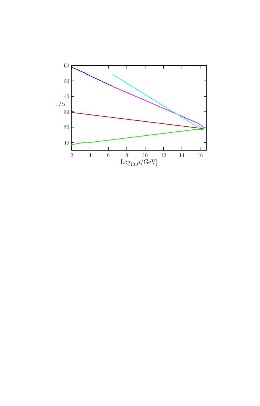
Figure 6: Unification picture for flipped $SU(5)\times U(1)$ model with $\alpha_{s}(M_{Z})\simeq 0.116$ and $\eta=0$; $M_{I}\simeq 2.8\cdot 10^{6}$ GeV, $\mu_{0}\simeq 4.7\cdot 10^{15}$ GeV, $M_{G}\simeq 2.8\cdot 10^{16}$ GeV.

where $M_{D}$ is the mass of $D^{(1)}$, $\overline{D}^{(2)}$ state’s zero modes. The mass scales, for which successful unification takes place in this model, are presented in Table 11. As we see, the masses of the doublets are in a range $1.7$ TeV–$141$ GeV. The picture of unification for the case in the last row of Table 11 is presented in Fig. 6.

Table 11: Unification for SUSY $G_{51}$ model. (Scales are measured in units of GeV.)

$$\begin{array}[]{|c|c|c|c|c|c|c|c|}\hline\cr M_{G}/\mu_{0}&(N,~{}N^{\prime})&\log_{10}[M_{I}]&\log_{10}[\mu_{0}]&\log_{10}[M_{G}]&\log_{10}[\frac{M_{I}}{M_{d^{c}_{H}}}]&\log_{10}[\frac{M_{I}}{M_{D}}]&\alpha_{3}(M_{Z})\\ \hline\cr\hline\cr 1&(0,~{}0)&15.37&16.37&16.37&12&12.15&0.119\\ \hline\cr 3&(0,~{}1)&14.59&15.61&16.09&11&12.2&0.1184\\ \hline\cr 4&(1,~{}1)&12.79&15.69&16.29&8&10.2&0.119\\ \hline\cr 5&(1,~{}2)&10.77&15.58&16.27&6.7&8.6&0.117\\ \hline\cr 6&(2,~{}2)&5.53&15.75&16.53&2&3.3&0.1176\\ \hline\cr 6&(2,~{}2)&6.45&15.67&16.45&3&4.3&0.116\\ \hline\cr\end{array}$$

Concluding this subsection, we note that in the flipped $SU(5)\times U(1)$ GUT it is impossible to get low scale (near few or multi TeV) unification. The reason is the following: introducing some additional states, one should cancel the positive power law contribution in (8.20) in order to get a reasonable $\alpha_{3}(M_{Z})$. The contribution from additional states will have the form $\frac{12}{7}{\Delta^{\prime}}_{2}-\frac{5}{7}{\Delta^{\prime}}_{1}-{\Delta^{\prime}}_{3}$, where ${\Delta^{\prime}}_{a}$ is a contribution to the renormalization of $\alpha^{-1}_{a}$. Since fragments from non trivial $SU(5)$ representations give the same contribution to factors of $SU(2)_{L}$ and $SU(3)_{c}$ we have ${\Delta^{\prime}}_{3}={\Delta^{\prime}}_{2}$. Therefore the final contribution to $\alpha_{3}^{-1}$ is $\frac{5}{7}({\Delta^{\prime}}_{2}-{\Delta^{\prime}}_{1})$. The latter should cancel the last two terms in (8.20), which in the $S_{1}=S_{2}\equiv S$ limit are equal to $\frac{12}{7\pi}S$. Thus, from the cancellation condition we have ${\Delta^{\prime}}_{1}-{\Delta^{\prime}}_{2}=\frac{12}{5\pi}S$; and thus the contribution in (8.21) is $\frac{6}{7}S$. This value precisely cancels the last two terms of (8.21) in the $S_{1}=S_{2}=S$ limit. This means that $M_{G}$ can not be lowered down to multi TeV. In Fig. 5 all couplings unify at one point. However, it would be quite natural in spirit of a two step unification that at a first step only the three couplings of $SU(5)$ unify and the $U(1)$ coupling joins at a higher scale. This can be achieved either by a change of the intermediate scale or by a different choice of the extra state’s masses.

9 Conclusions and outlook

We have considered 5D orbifold SUSY models and within them we have addressed numerous phenomenological issues. Orbifold constructions give an attractive resolution of several outstanding problems of GUTs, but some extensions are still needed to have full control of difficulties which even appear outside GUTs. In fact, problems such as baryon number violation, $\mu$ problem and neutrino oscillations (tied with lepton number violation) are not cured by extra dimensions, and some care is needed to deal with them. In our approach we have considered extensions with a discrete ${\cal Z}$ symmetry, which gives a natural and simultaneous understanding of these problems. In the essential part of the paper we have addressed the question of gauge coupling unification, which in the presence of KK states gets new facets. Since the orbifold approach to the celebrated $SU(5)$ GUT does not allow for low or intermediate scale unification, we studied extended (in rank) GUTs. As we have seen this opens up new and interesting possibilities from the viewpoints of unification and phenomenological implications. For extended GUTs, symmetry breaking can occur by a step by step compactification and if the intermediate gauge group differs from semisimple $SU(5)$, power law unification can take place. As an example we have considered the two maximal subgroups of $SO(10)$ - the Pati-Salam $G_{422}$ and flipped $G_{51}$ GUTs. Within $G_{422}$, low scale unification can take place, while $G_{51}$ only allows for unification at scales $\sim 10^{16}$ GeV. The latter scales are also possible for $G_{422}$. Within both scenarios extensions with a discrete ${\cal Z}$ symmetry were pursued; thus key phenomenological problems were resolved in an elegant way. The $G_{51}$ model and also in some cases the $G_{422}$ one predict colored triplet states in the few TeV range. $G_{422}$ models with low scale unification lead to additional relatively light states. Because of these the models have an interesting phenomenology, in particular if KK states appear near the TeV scale. Future high energy collider experiments will test the relevance of such models.

In our studies we have used one loop RGE analysis. Two loop power law contributions to the $\beta$-function would contribute significantly. This would make estimates unstable. However, due to higher dimensional supersymmetries, in higher loops full sets of $N=2$ supermultiplets can contribute [29], [30] and in this case effects of higher loops will be logarithmic. The latter contributions would not change the unification picture and might only imply a slight modification of mass scales. The same argument could be applied for threshold corrections coming from different sources.

Our studies of the $G_{422}$ and $G_{51}$ groups were performed in a bottom-up approach and therefore the ’low energy’ sector was more relevant for our considerations. Having in mind that both $G_{422}$ and $G_{51}$ are maximal subgroups of $SO(10)$, it would be interesting to construct a higher (at least two extra) dimensional $SO(10)$ model where extra dimensions do not compactify at a single mass scale (in contrast to the models of [22]) but with intermediate groups $G_{422}$ or $G_{51}$ at a scale between $\frac{1}{R^{\prime}}\gg\frac{1}{R}$. Only this kind of step by step compactification breaking of an initial semisimple gauge group can give power law unification near the TeV scale. It would be also interesting to consider other extended gauge groups in higher dimensions and to study the breaking pattern and the phenomenological implications. We wish to study these and other relevant issues in our future publications.

Acknowledgement

F.P.C. is supported by Fundação de Ciência e Tecnologia (grant SFRH/BD/4973/2001).

Appendix A: Influence of brane couplings
        on gauge coupling unification

In this appendix we investigate the influence of some brane operators on gauge coupling renormalization. We will show that the 4D mass term of bulk vectorlike states does not change the expressions for the power law functions $S$ and $S_{1}$, $S_{2}$ of (3.8) and (3.10) resp.. Also, it turns out that some brane bi-linear derivative couplings, involving states with negative parities, do not change this picture for $\mu_{0}\ll M\sim M_{G}$. The latter condition is usually satisfied in models with power law unification . Our discussion will be model independent. We will consider here the case of $S^{(1)}/Z_{2}$ orbifold, but generalization to $S^{(1)}/Z_{2}\times Z_{2}^{\prime}$ scenarios is straightforward.

Consider two $N=2$ supermultiplets ${\bf E}_{N=2}=(E,~{}\overline{E})$ and ${\bf E^{\prime}}_{N=2}=(E^{\prime},~{}{\overline{E}}^{\prime})$ transforming non trivially under a certain gauge group $G$. If $E$, $E^{\prime}$ belong to some representation ${\bf r}$ of $G$, then $\overline{E}$, ${\overline{E}}^{\prime}$ transform as ${\bf\bar{r}}$. Let us assign the orbifold parities as

$$(E,~{}{\overline{E}}^{\prime})\sim{\bf+}~{},~{}~{}~{}~{}(E^{\prime},~{}\overline{E})\sim{\bf-}~{}.$$ (A.1)

Thus, only $E$, ${\overline{E}}^{\prime}$ states have zero modes. Writing the brane coupling

$$\int d^{5}xd^{2}\theta\delta(y)\left(\lambda_{E}\,E{\overline{E}}^{\prime}+h.c.\right)~{},$$ (A.2)

we obtain, after performing the integration over $y$, the 4D superpotential mass terms

$$W_{E}=2M_{E}\sum_{m,n}E^{(m)}{\overline{E}^{(n)}}^{\prime}\eta^{(m)}\eta^{(n)}~{},$$ (A.3)

where $M_{E}=\lambda_{E}\mu_{0}/\pi=\lambda_{E}/(\pi R)$ and $\eta^{(0)}=1/\sqrt{2}$, $\eta^{(n)}|_{n\neq 0}=1$. On the other hand, the last term in the 5D bulk Lagrangian (2.4) gives direct mass terms for the KK states

$$W^{KK}_{E}=\mu_{0}\sum_{n=1}^{\infty}n\left(E^{(n)}\overline{E}^{(n)}+{E^{(n)}}^{\prime}{\overline{E}^{(n)}}^{\prime}\right)~{}.$$ (A.4)

For our calculations only a certain number of KK states is relevant, which contribute to the gauge coupling runnings. So, we truncate the tower of KK states on the level $N_{0}$. Taking this into account and combining (A.3), (A.4), the mass terms can be written in compact form as

$$W_{E}+W^{KK}_{E}=\overline{{\mathcal{E}}}{\mathcal{M}}{\mathcal{E}}~{},$$ (A.5)

where

$$\overline{{\mathcal{E}}}=\left(~{}\bar{E}^{\prime(N)}~{}\ldots~{}\bar{E}^{\prime(0)}~{}\bar{E}^{(1)}~{}\ldots~{}\bar{E}^{(N)}~{}\right),~{}~{}{\mathcal{E}}^{T}=\left(~{}E^{\prime(N)}~{}\ldots~{}E^{\prime(1)}~{}E^{(0)}~{}\ldots~{}E^{(N)}~{}\right),$$ (A.6)

$${\mathcal{M}}\equiv\left[\begin{array}[]{cc}\bar{{\mathcal{M}}}_{0}&{\mathcal{M}}_{E}\\ 0&{\mathcal{M}}_{0}\end{array}\right],\quad{\mathcal{M}}_{E}=M_{E}\left[\begin{array}[]{cccc}\sqrt{2}&2&\ldots&2\\ \vdots&&\ddots&\vdots\\ \sqrt{2}&2&\ldots&2\\ 1&\sqrt{2}&\ldots&\sqrt{2}\end{array}\right]~{},$$ (A.7)

and

$$\bar{{\mathcal{M}}}_{0}=\mu_{0}\left[\begin{array}[]{cccc}N_{0}&0&\ldots&0\\ 0&N_{0}-1&&0\\ \vdots&&\ddots&\vdots\\ 0&0&\ldots&1\\ 0&0&\ldots&0\end{array}\right],\qquad{\mathcal{M}}_{0}=\mu_{0}\left[\begin{array}[]{ccccc}0&1&\ldots&0&0\\ \vdots&&\ddots&&\vdots\\ 0&0&&N_{0}-1&0\\ 0&0&\ldots&0&N_{0}\end{array}\right]~{}.$$ (A.8)

To estimate the KK and zero mode contributions to the running, one should diagonalize the matrix ${\mathcal{M}}$ and find the eigenvalues $M_{0}$, $M_{1}$, $\cdots$, $M_{2N_{0}}$. If all these masses lie below $M_{G}$, then their contribution to the renormalization of $\alpha_{i}^{-1}$ up to the GUT scale will be

$$\Delta^{E}_{i}=-\frac{b_{i}^{E}}{2\pi}\sum_{n=0}^{2N_{0}}\ln\frac{M_{G}}{M_{n}}=-\frac{b_{i}^{E}}{2\pi}\ln\frac{M_{G}^{2N_{0}+1}}{{\rm det}{\mathcal{M}}}~{}.$$ (A.9)

From (A.7), (A.8) it is easy to see that

$${\rm det}{\mathcal{M}}=M_{E}\left(\prod_{n=1}^{N_{0}}M_{n}\right)^{2}=M_{E}\left(\prod_{n=1}^{N_{0}}n\mu_{0}\right)^{2}~{}.$$ (A.10)

Using (A.10) in (A.9) we obtain

$$\Delta^{E}_{i}=-\frac{b^{E}_{i}}{2\pi}\ln\frac{M_{G}}{M_{E}}--\frac{\hat{b}^{E}_{i}}{2\pi}\sum_{n=1}^{N_{0}}\ln\frac{M_{G}}{n\mu_{0}}~{},$$ (A.11)

(where we have set $\hat{b}^{E}_{i}=2b^{E}_{i}$). As one can see, the first term in (A.11) is just the naive logarithmic running of ’zero mode’ states, while the second term has precisely the form of the ’unaffected’ KK power law running (3.8). From this we conclude that due to the brane coupling (A.2), the RGEs will in addition include a logarithmic term corresponding to the zero modes $E^{(0)}$, ${\overline{E}^{(0)}}^{\prime}$ above the scale $M_{E}$, while the effect of the KK states must be estimated by the power law function $S$. These conclusions are valid for any value of $M_{E}\stackrel{{\scriptstyle<}}{{{}_{\sim}}}M_{G}$.

Higher order brane couplings, preserving orbifold symmetries, imply $\partial_{5}$ derivatives and must be cut off at the fundamental scale $M\sim M_{G}$. For example, the couplings

$$\int d^{5}xd^{2}\theta\delta(y)\left(\frac{1}{M}E\partial_{5}\overline{E}+\frac{1}{M}{\overline{E}}^{\prime}\partial_{5}E^{\prime}\right)~{},$$ (A.12)

after integration along the fifth dimension, change the masses by the amount $\sim\mu_{0}^{2}/M$. The latter is negligible for $\mu_{0}\ll M$ and (A.11) is still valid.

Figure 1: Unification picture for model I-susy422 with $\alpha_{s}(M_{Z})\simeq 0.119$ and $\eta=0$; $M_{I}\simeq 8.5\cdot 10^{10}$ GeV, $\mu_{0}\simeq 1.4\cdot 10^{11}$ GeV, $M_{G}\simeq 4.3\cdot 10^{12}$ GeV.

References

- [1] H. Georgi, S.L. Glashow, Phys.Rev.Lett. 32 (1974) 438; H. Fritzsch, P. Minkowski, Ann. Phys. 93 (1975) 193.
- [2] H. Georgi, H. Quinn, S. Weinberg, Phys. Rev. Lett. 33 (1974) 451; W. Marciano, A. Sirlin, Phys. Rev. Lett. 46 (1981) 163.
- [3] J. Ellis, S. Kelley, D. Nanopoulos, Phys. Lett. B 260 (1991) 131;
- [4] S. Dimopoulos, H. Georgi, Nucl. Phys. B 193 (1981) 150; N. Sakai, Z. Phys. C 11 (1982) 153.
- [5] S. Dimopoulos, S. Raby, F. Wilczek, Phys. Rev. D 24 (1981) 1681; W. Marciano, G. Senjanovic, Phys. Rev. D 25 (1982) 3092.
- [6] D.R.T. Jones, Phys.Rev. D 25 (1982) 581.
- [7] C. Giunti, C. Kim, U. Lee, Mod. Phys. Lett. A 6 (1991) 1745; P. Langacker, M. Luo, Phys. Rev. D 44 (1991) 817.
- [8] U. Amaldi, W. de Boer, H. Furstenau, Phys. Lett. B 260 (1991) 447.
- [9] Particle Data Group, Eur. Phys. J. C 15 (2000) 1.
- [10] R. Arnowitt, P. Nath, Phys. Lett. B 287 (1992) 89; Phys. Rev. Lett. 70 (1993) 3696; J. Hisano, H. Murayama, T. Yanagida, Nucl. Phys. B 402 (1993) 46; K.S. Babu, S.M. Barr, Phys. Lett. B 381 (1996) 137; Z. Berezhiani, Z. Tavartkiladze, M. Vysotsky, hep-ph/9809301; R. Dermisek, A. Mafi, S. Rabi, Phys. Rev. D 63 (2001) 035001; H. Murayama, A. Pierce, hep-ph/0108104.
- [11] S. Fukuda et al. [Super-Kamiokande Collaboration], Phys. Rev. Lett. 88 (2000) 3999; N. Fornengo et al., Nucl. Phys. B 580 (2000) 58.
- [12] S. Fukuda et al. [Super-Kamiokande Collaboration], Phys. Rev. Lett. 86 (2001) 5651; J. Bahcall, P. Krastev, A. Smirnov, hep-ph/0006078; M.C. Gonzalez-Garcia et al., Nucl. Phys. B 573 (2000) 3.
- [13] I. Antoniadis, J. Ellis, S. Kelley, D. Nanopoulos, Phys.Lett. B 272 (1991) 31. P. Lamgacker, N. Polonsky, Phys. Rev. D 47 (1993) 4028; Phys. Rev. D 52 (1995) 52; N. Polonsky, hep-ph/0108236; see also references terein.
- [14] M. Shifman, Mod. Phys. Lett. A 10 (1995) 605; J. Bagger, K. Matchev, D. Pierce, Phys. Lett. B 348 (1995) 443.
- [15] Y. Kawamura, Prog. Theor. Phys. 105 (2001) 999; ibid. 105 (2001) 691.
- [16] G. Altarelli, F. Feruglio, hep-ph/0102301; A. Kobakhidze, hep-ph/0102323; M. Kakizaki, M. Yamaguchi, hep-ph/0104103; N. Maru, hep-ph/0108002.
- [17] Y. Nomura, D. Smith, N. Weiner, hep-ph/0104041; T. Kawamoto, Y. Kawamura, hep-ph/0106163; R. Barbieri, L. Hall, Y. Nomura, hep-th/0107004; A. Hebecker, J. March-Russell, hep-ph/0107039; C. Csaki, G. Kribs, J. Terning, hep-ph/0107266.
- [18] Q. Shafi, Z. Tavartkiladze, hep-ph/0108247.
- [19] T. Li, hep-ph/0108120; hep-th/0110065; M. Chaichian, J. Chkareuli, A. Kobakhidze, hep-ph/0108131; C.S. Huang, J. Jiang, T. Li, hep-th/0112046; K.S. Babu, S.M. Barr, B. Kyae, hep-ph/0202178.
- [20] L. Hall, Y. Nomura, hep-ph/0103125; hep-ph/0205067.
- [21] A. Hebecker, J. March-Russell, hep-ph/0106166; H. Cheng, K. Matchev, J. Wang, hep-ph/0107268; L. Hall, J. March-Russell, T. Okui, D. Smith, hep-ph/0108161; Y. Nomura, hep-ph/0108170.
- [22] T. Asaka, W. Buchmüller, L. Covi, hep-ph/0108021; L. Hall, Y. Nomura, T. Okui, D. Smith, hep-ph/0108071; R. Dermisek, A. Mafi, hep-ph/0108139; N. Haba, T. Kondo, Y. Shimizu, hep-ph/0112132, hep-ph/0202191.
- [23] R. Blumenhagen, L. Goerlich, B. Körs, D. Lüst, hep-th/0010198; G. Aldazabal, S. Franco, L. Ibanez, R. Rabadan, A. Uranga, hep-th/0011073; hep-ph/0011132; L.E. Ibanez, F. Marchesano, R. Rabadan, hep-th/0105155; R. Blumenhagen, B. Körs, D. Lüst, T. Ott, hep-th/0107138.
- [24] I. Antoniadis, Phys. Lett. B 246 (1990) 377; I. Antoniadis, C. Munoz, M. Quiros, Nucl. Phys. B 397 (1993) 515; J. Lykken, Phys. Rev. D 54 (1996) 3693; I. Antoniadis, S. Dimopoulos, A. Giveon, hep-th/0103033.
- [25] I. Antoniadis, K. Benakli, M. Quiros, Phys. Lett. B 331 (1994) 313; hep-ph/9905311; I. Antoniadis, K. Benakli, hep-ph/0007226; and references therein.
- [26] For recent reviews see J. Polchinski, hep-th/9611050; C. Vafa, hep-th/9702201; A. Sen, hep-th/9802051; I. Antoniadis, G. Ovarlez, hep-th/9906108; I. Antoniadis, hep-th/0102202.
- [27] N. Arkani-Hamed, S. Dimopoulos, G. Dvali, Phys. Lett. B 429 (1998) 263; Phys. Rev. D 59 (1999) 086004; I. Antoniadis, N. Arkani-Hamed, S. Dimopoulos, G. Dvali, Phys. Lett. B 436 (1998) 257.
- [28] J. Price, proc. Int. Symp. on Experimental Gravitational Physics, ed. P. Michelson, Guangzhou, China (World Sci., Singapore 1988); J. Price et al., NSF proposal 1996; A. Kapitulnik, T. Kenny, NSF proposal, 1997; J. Long et al., hep-ph/9805217.
- [29] K. Dines, E. Dudas, T. Gherghetta, Phys. Lett. B 436 (1998) 55; Nucl. Phys. B 537 (1999) 47.
- [30] Z. Kakushadze, Nucl. Phys. B 548 (1999) 205; ibid. B 552 (1999) 3.
- [31] C. Carone, hep-ph/9902407; A. Delgado, M. Quiros, hep-ph/9903400; P. Frampton, A. Rasin, hep-ph/9903479; A. Perez-Lorenzana, R.N. Mohapatra, hep-ph/9904504; Z. Tavartkiladze, hep-ph/0105281.
- [32] T. Kobayashi, J. Kubo, M. Mondragon, G. Zoupanos, Nucl. Phys. B 550 (1999) 99; K. Huitu, T. Kobayashi, Phys. Lett. B 470 (1999) 90.
- [33] T. Taylor, G. Veneziano, Phys. Lett. B 212 (1988) 147.
- [34] J. Pati, A. Salam, Phys. Rev. D 10 (1974) 275.
- [35] S. Barr, Phys. Lett. B 112 (1982) 219.
- [36] R. Slansky, Phys. Rept. 79 (1981) 1.
- [37] M. Sohnius, Phys. Rep. 128 (1985) 39; A. Salam, E. Sezgin, V. 1, 2, World Scientific, 1989; E. Mirabelli, M. Peskin, hep-th/9712214.
- [38] N. Arkani-Hamed, T. Gregoire, J. Wacker, hep-th/0101233; D. Marti, A. Pomarol, hep-th/0106256; A. Hebecker, hep-ph/0112230.
- [39] L. Ibanez, G. Ross, Nucl. Phys. B 368 (1992) 3.
- [40] I. Antoniadis, J. Hagelin, D. Nanopoulos, Phys. Lett. B 194 (1987) 231; G. Lazarides, C. Panagiotakopoulos, Q. Shafi, Phys. Lett. B 315 (1993) 325; G. Dvali, Q. Shafi, Phys. Lett. B 403 (1997) 65; Q. Shafi, Z. Tavartkiladze, hep-ph/9811282; hep-ph/9807502.
- [41] I. Antoniadis, hep-th/0102202.
- [42] C. Carone, H. Murayama, Phys. Rev. D 52 (1995) 484; D. Bailey, S. Davidson, hep-ph/9411355.
- [43] G. Dvali, Q. Shafi, Phys. Lett. B 326 (1994) 258; B 339 (1994) 241. J.E. Kim, H.P. Nilles, Mod. Phys. Lett. A 38 (1994) 3575. K. Choi, E.J. Chun, H. Kim, Phys. Rev. D 55 (1997) 7010.
- [44] G. Dvali, Q. Shafi, Phys.Lett. B 339 (1994) 241; Z. Berezhiani, C. Csaki, L. Randall, hep-ph/9501336; see also Q. Shafi, Z. Tavartkiladze, in ref. [40].
- [45] G. Bhattacharyya, Nucl. Phys. Proc. Suppl. A 52 (1997) 83; J.C. Romao, hep-ph/9811454.
- [46] T. Banks, Y. Grossman, E. Nardi, Y. Nir, Phys. Rev. D 52 (1995) 5319.
- [47] H. Nilles, N. Polonsky, Nucl. Phys. B 484 (1997) 33; E. Nardi, Phys. Rev. D 55 (1997) 5772; G. Eyal, Y. Nir, hep-ph/9904473; J. Chkareuli, I. Gogoladze, A. Kobakhidze, M. Green, D. Hutchcroft, hep-ph/9908451; Q. Shafi, Z. Tavartkiladze, hep-ph/9909238; J. Feng, Y. Nir, Y. Shadmi, hep-ph/9911370; see also other references therein.
- [48] R. Hempfling, Nucl. Phys. B 478 (1996) 3; E.J. Chun, S.K. Kang, hep-ph/9909429.
- [49] M. Carena, T. Tait, C. Wagner, hep-ph/0207056, M. Chaichian, A. Kobakhidze, hep-ph/0208129.
- [50] D. Caldwell, R. Mohapatra, Phys. Rev. D 48 (1993) 3259; C. Carone, M. Sher, hep-ph/9711259; F. Vissani, hep-ph/9708483; H. Georgi, S. Glashow, hep-ph/9808293; Y.L. Wu, hep-ph/9810491; C. Wetterich, hep-ph/9812426; J. Ellis, S. Lola, hep-ph/9904279; see also references therein.
- [51] J. Elwood, N. Irges, P. Ramond, hep-ph/9807228; F. Vissani, hep-ph/9810435; Z. Berezhiani, A. Rossi, hep-ph/9811447; R. Barbieri, L. Hall, G. Kane, G. Ross, hep-ph/9901228; Q. Shafi, Z. Tavartkiladze, hep-ph/9901243; hep-ph/0002150; G. Altarelli, F. Feruglio, I. Masina, hep-ph/9907532; S. Barr, I. Dorsner, hep-ph/0003058; J. Chkareuli, C. Froggatt, H. Nielsen, hep-ph/0109156; I. Gogoladze, A. Perez-Lorenzana, hep-ph/0112034; F. Feruglio, A. Strumia, F. Vissani, hep-ph/0201291; see also references therein.
- [52] G. Dvali, M. Shifman, Phys. Lett. B 399 (1997) 60.
- [53] G. Abbiendi et al. [OPAL Collaboration], Eur. Phys. J. C 12 (2000) 1; M. Carena, G. Giudice, S. Lola, C. Wagner, hep-ph/9612334; B. Mukhopadhyaya, S. Roy, hep-ph/9903418.
- [54] M.E. Pospelov, Phys. Rev. D 56 (1997) 259.