The Crystallography of Color Superconductivity

We develop the Ginzburg-Landau approach to comparing different possible crystal structures for the crystalline color superconducting phase of QCD, the QCD incarnation of the Larkin-Ovchinnikov-Fulde-Ferrell phase. In this phase, quarks of different flavor with differing Fermi momenta form Cooper pairs with nonzero total momentum, yielding a condensate that varies in space like a sum of plane waves. We work at zero temperature, as is relevant for compact star physics. The Ginzburg-Landau approach predicts a strong first-order phase transition (as a function of the chemical potential difference between quarks) and for this reason is not under quantitative control. Nevertheless, by organizing the comparison between different possible arrangements of plane waves (i.e. different crystal structures) it provides considerable qualitative insight into what makes a crystal structure favorable. Together, the qualitative insights and the quantitative, but not controlled, calculations make a compelling case that the favored pairing pattern yields a condensate which is a sum of eight plane waves forming a face-centered cubic structure. They also predict that the phase is quite robust, with gaps comparable in magnitude to the BCS gap that would form if the Fermi momenta were degenerate. These predictions may be tested in ultracold gases made of fermionic atoms. In a QCD context, our results lay the foundation for a calculation of vortex pinning in a crystalline color superconductor, and thus for the analysis of pulsar glitches that may originate within the core of a compact star.

1 Introduction

Since quarks that are antisymmetric in color attract, cold dense quark matter is unstable to the formation of a condensate of Cooper pairs, making it a color superconductor [1, 2, 3, 4, 5]. At asymptotic densities, the ground state of QCD with quarks of three flavors ($u$, $d$ and $s$) is expected to be the color-flavor locked (CFL) phase [6, 5]. This phase features a condensate of Cooper pairs of quarks that includes $ud$, $us$, and $ds$ pairs. Quarks of all colors and all flavors participate in the pairing, and all excitations with quark quantum numbers are gapped. As in any BCS state, the Cooper pairing in the CFL state pairs quarks whose momenta are equal in magnitude and opposite in direction, and pairing is strongest between pairs of quarks whose momenta are both near their respective Fermi surfaces.

Pairing persists even in the face of a stress (such as a chemical potential difference or a mass difference) that seeks to push the quark Fermi surfaces apart, although a stress that is too strong will ultimately disrupt BCS pairing. The CFL phase is the ground state for real QCD, assumed to be in equilibrium with respect to the weak interactions, as long as the density is high enough. Now, imagine decreasing the quark number chemical potential $\mu$ from asymptotically large values. The quark matter at first remains color-flavor locked, although the CFL condensate may rotate in flavor space as terms of order $m_{s}^{4}$ in the free energy become important [7]. Color-flavor locking is maintained until an “unlocking transition”, which must be first order [8, 9], occurs when [8, 9, 10, 11, 12]

$$\mu\approx m_{s}^{2}/4\Delta_{0}\ .$$ (1.1)

In this expression, $\Delta_{0}$ is the BCS pairing gap, estimated in both models and asymptotic analyses to be of order tens to 100 MeV [5], and $m_{s}$ is the strange quark mass parameter. Note that $m_{s}$ includes the contribution from any $\langle\bar{s}s\rangle$ condensate induced by the nonzero current strange quark mass, making it a density-dependent effective mass. At densities that may occur at the center of compact stars, corresponding to $\mu\sim 400-500$ MeV, $m_{s}$ is certainly significantly larger than the current quark mass, and its value is not well known. In fact, $m_{s}$ decreases discontinuously at the unlocking transition [13]. Thus, the criterion (1.1) can only be used as a rough guide to the location of the unlocking transition in nature [13, 12]. Given this quantitative uncertainty, there remain two logical possibilities for what happens as a function of decreasing $\mu$. One possibility is a first-order phase transition directly from color-flavor locked quark matter to hadronic matter, as explored in Ref. [11]. The second possibility is an unlocking transition, followed only at a lower $\mu$ by a transition to hadronic matter. We assume the second possibility here, and explore its consequences.

One may think that $ud$ BCS pairing could persist below the unlocking transition. However, this does not occur in electrically neutral bulk matter [12]. The unlocking transition is a transition from the CFL phase to “unpaired” quark matter in which electrical neutrality is enforced by an electrostatic potential $\mu_{e}\sim m_{s}^{2}/4\mu$, to lowest order in $m_{s}/\mu$, meaning that the Fermi momenta are related (to this order) by

$$p_{F}^{d} = p_{F}^{u}+\frac{m_{s}^{2}}{4\mu}$$

$$p_{F}^{s} = p_{F}^{u}-\frac{m_{s}^{2}}{4\mu}\ .$$ (1.2)

If this “unpaired” quark matter exists in some window of $\mu$ between hadronic matter and CFL quark matter, there will be pairing in this window: all that Ref. [12] shows is that there will be no BCS pairing between quarks of different flavors. One possible pattern of pairing is the formation of $\langle uu\rangle$, $\langle dd\rangle$ and $\langle ss\rangle$ condensates. These must be either $J=1$ or symmetric in color, whereas the QCD interaction favors the formation of color antisymmetric $J=0$ pairs. The gaps in these phases may be as large as of order 1 MeV [14], or could be much smaller [3]. Another possibility for pairing in the “unpaired” quark matter is crystalline color superconductivity [15, 16, 17, 18, 19, 20], which involves pairing between quarks whose momenta do not add to zero, as first considered in a terrestrial condensed matter physics context by Larkin, Ovchinnikov, Fulde and Ferrell (LOFF) [21, 22]. Unpaired quark matter with Fermi momenta (1.2) is susceptible to the formation of a crystalline color superconducting condensate constructed from pairs of quarks that are antisymmetric in color and flavor, where both quarks have momenta near their respective unpaired Fermi surfaces. We shall argue in this paper that the crystalline color superconducting phase is more robust than previously thought, with gaps comparable to $\Delta_{0}$. In fact, crystalline color superconducting pairing lowers the free energy so much that its pairing energy should be taken into account in the comparison (1.1). This comparison should be redone as a competition between the crystalline color superconducting and CFL phases: crystalline color superconductivity in the “unpaired” quark matter is sufficiently robust that it will delay the transition to the CFL phase to a significantly higher density than that in (1.1).

The idea behind crystalline color superconductivity is that once CFL pairing is disrupted, leaving quarks with differing Fermi momenta that are unable to participate in BCS pairing, it is natural to ask whether there is some generalization of the pairing ansatz in which pairing between two species of quarks persists even once their Fermi momenta differ. It may be favorable for quarks with differing Fermi momenta to form pairs whose momenta are not equal in magnitude and opposite in sign [21, 22, 15]. This generalization of the pairing ansatz (beyond BCS ansätze in which only quarks with momenta which add to zero pair) is favored because it gives rise to a region of phase space where both of the quarks in a pair are close to their respective Fermi surfaces, and such pairs can be created at low cost in free energy. Condensates of this sort spontaneously break translational and rotational invariance, leading to gaps that vary in a crystalline pattern.

Crystalline color superconductivity may occur within compact stars. With this context in mind, it is appropriate for us to work at zero temperature because compact stars that are more than a few minutes old are several orders of magnitude colder than the tens-of-MeV-scale critical temperatures for BCS or crystalline color superconductivity. As a function of increasing depth in a compact star, $\mu$ increases, $m_{s}$ decreases, and $\Delta_{0}$ changes also. This means that in some shell within the quark matter core of a neutron star (or within a strange quark star), $m_{s}^{2}/\mu\Delta_{0}$ may lie within the appropriate window where crystalline color superconductivity is favored. Because this phase is a (crystalline) superfluid, it will be threaded with vortices in a rotating compact star. Because these rotational vortices may pinned in place by features of the crystal structure, such a shell may be a locus for glitch phenomena [15].

To date, crystalline color superconductivity has only been studied in simplified models with pairing between two quark species whose Fermi momenta are pushed apart by a chemical potential difference [15, 16, 17, 18, 20] or a mass difference [19]. We suspect that in reality, in three-flavor quark matter whose unpaired Fermi momenta are split as in (1.2), the color-flavor pattern of pairing in the crystalline phase will involve $ud$, $us$ and $ds$ pairs, just as in the CFL phase. Our focus here, though, is on the form of the crystal structure. That is, we wish to focus on the dependence of the crystalline condensate on position and momenta. As in previous work, we therefore simplify the color-flavor pattern to one involving massless $u$ and $d$ quarks only, with Fermi momenta split by introducing chemical potentials

$$\mu_{d} = \bar{\mu}+\delta\mu$$

$$\mu_{u} = \bar{\mu}-\delta\mu\ .$$ (1.3)

In this toy model, we vary $\delta\mu$ by hand. In three-flavor quark matter, the analogue of $\delta\mu$ is controlled by the nonzero strange quark mass and the requirement of electrical neutrality and would be of order $m_{s}^{2}/4\mu$ as in (1.2).

In our toy model, we shall take the interaction between quarks to be pointlike, with the quantum numbers of single-gluon exchange. This $s$-wave interaction is a reasonable starting point at accessible densities but is certainly inappropriate at asymptotically high density, where the interaction between quarks (by gluon exchange) is dominated by forward scattering. The crystalline color superconducting state has been analyzed at asymptotically high densities in Refs. [18, 20]. As we shall explain, the analysis of Ref. [18] indicates that the crystal structure in this circumstance would be different from that we obtain.

Our toy model may turn out to be a better model for the analysis of LOFF pairing in atomic systems. (There, the phenomenon could be called “crystalline superfluidity”.) Recently, ultracold gases of fermionic atoms have been cooled down to the degenerate regime, with temperatures less than the Fermi energy [23], and reaching the pairing transition (perhaps by increasing the atom-atom interaction rather than by further reducing the temperature) seems a reasonable possibility [24]. In such systems, there really are only two species of atoms (two spin states) that pair with each other, whereas in QCD our model is a toy model for a system with nine quarks. In the atomic systems, the interaction will be $s$-wave dominated whereas in QCD, it remains to be seen how good this approximation is at accessible densities. Furthermore, in the atomic physics context experimentalists can control the densities of the two different atoms that pair, and in particular can tune their density difference. This means that experimentalists wishing to search for crystalline superfluidity have the ability to dial the most relevant control parameter [25, 26]. In QCD, in contrast, $\delta\mu$ is controlled by $m_{s}^{2}/\mu$, meaning that it is up to nature whether, and if so at what depth in a compact star, crystalline color superconductivity occurs.

In the simplest LOFF state, each Cooper pair carries momentum $2{\bf q}$. Although the magnitude $|{\bf q}|$ is determined energetically, the direction $\hat{\bf q}$ is chosen spontaneously. The condensate is dominated by those regions in momentum space in which a quark pair with total momentum $2{\bf q}$ has both members of the pair within of order $\Delta$ of their respective Fermi surfaces. These regions form circular bands on the two Fermi surfaces, as shown in Fig. 1. Making the ansatz that all Cooper pairs make the same choice of direction $\hat{\bf q}$ corresponds to choosing a single circular band on each Fermi surface, as in Fig. 1. In position space, it corresponds to a condensate that varies in space like

$$\langle\psi({\bf x})\psi({\bf x})\rangle\propto\Delta e^{2i{\bf q}\cdot{\bf x}}\ .$$ (1.4)

This ansatz is certainly not the best choice, because it only allows a small fraction of all the quarks near their Fermi surfaces to pair. If a single plane wave is favored, why not two? That is, if one choice of $\hat{\bf q}$ is favored, why not add a second ${\bf q}$, with the same $|{\bf q}|$ but a different $\hat{\bf q}$, to allow more quarks near their Fermi surfaces to pair? If two are favored, why not three? Why not eight? If eight plane waves are favored, how should their $\hat{\bf q}$’s be oriented? These are the sort of questions we seek to answer in this paper.

\psfrag{muu}[r][r]{$\mu_{u}$}\psfrag{mud}[l][l]{$\mu_{d}$}\psfrag{p}[l][l]{${\mathbf{p}}$}\psfrag{mp}[r][r]{$-{\mathbf{p}}$}\psfrag{p2q}[r][r]{$-{\mathbf{p}}+2{\mathbf{q}}$}\psfrag{pp}[r][r]{${\mathbf{p}}^{\prime}$}\psfrag{mpp}[l][l]{$-{\mathbf{p}}^{\prime}$}\psfrag{pp2q}[l][l]{$-{\mathbf{p}}^{\prime}+2{\mathbf{q}}$}\psfrag{2q}[c][c]{$2{\mathbf{q}}$}\psfrag{psiu}[c][l]{$\psi_{u}$}\psfrag{psid}[c][l]{$\psi_{d}$}\includegraphics[width=252.94499pt]{rings.eps}

Figure 1: In the simplest LOFF state, in which every Cooper pair carries momentum $2{\bf q}$, an up quark with momentum ${\mathbf{p}}$ (or ${\mathbf{p}}^{\prime}$) pairs with a down quark with momentum $-{\mathbf{p}}+2{\mathbf{q}}$ (or $-{\mathbf{p}}^{\prime}+2{\mathbf{q}}$). In the figure ${\mathbf{q}}$ has been taken to point upwards. The pairing is dominated by pairing between up quarks in a band centered on the dashed ring shown on the up Fermi surface, and down quarks in a band centered on the solid ring shown on the down Fermi surface. The vector sum of the momenta in any pair is $2{\mathbf{q}}$, and the pairing bands are defined as those pairs such that both quarks in a pair are within $\Delta$ of their respective Fermi surface. The thickness of the pairing bands is thus of order $\Delta$. The width of the pairing bands is of order $\Delta\bar{\mu}/{\delta\mu}$, meaning that their angular width is of order $\Delta/{\delta\mu}$. We take a weak coupling limit in which $\Delta_{0}\rightarrow 0$ while ${\delta\mu}/\Delta_{0}$ and $|{\mathbf{q}}|/\Delta_{0}$ are held fixed and nonzero. In this limit, $\Delta/\Delta_{0}$ also stays fixed, and therefore so does the angular width of the pairing bands. In this limit, the two Fermi surfaces in the figure get closer and closer together and the angles $\psi_{u}$ and $\psi_{d}$ become degenerate, and take on the value $\psi_{0}=2\cos^{-1}({\delta\mu}/|{\mathbf{q}}|)\simeq 67.1^{\circ}$. If, in addition, we take the further limit in which ${\delta\mu}/\Delta_{0}\rightarrow{\delta\mu}_{2}/\Delta_{0}$, approaching the second-order phase transition, then in this Ginzburg-Landau limit the angular extent of the pairing bands shrinks to zero, reducing them to only the rings shown.

Upon making the plane-wave ansatz (1.4), we know from previous work [21, 22, 27, 15] that this simplest LOFF phase is favored over the BCS state and over no pairing at all in a range $\delta\mu_{1}<\delta\mu<\delta\mu_{2}$, where ${\delta\mu}_{1}=\Delta_{0}/\sqrt{2}\simeq 0.707\Delta_{0}$ and ${\delta\mu}_{2}\simeq 0.754\Delta_{0}$. At $\delta\mu_{2}$, there is a second-order phase transition at which $\Delta/\Delta_{0}\rightarrow 0$ and $|{\bf q}|/\Delta_{0}$ tends to a nonzero limit, which we shall denote $q_{0}/\Delta_{0}$, where $q_{0}\simeq 0.90\Delta_{0}\simeq 1.2\delta\mu_{2}$. At the second-order phase transition, the quarks that participate in the crystalline pairing lie on circular rings on their Fermi surfaces that are characterized by an opening angle $\psi_{0}=2\cos^{-1}({\delta\mu}/|{\mathbf{q}}|)\simeq 67.1^{\circ}$ and an angular width that is of order $\Delta/{\delta\mu}$, which therefore tends to zero. At $\delta\mu_{1}$ there is a first-order phase transition at which the LOFF solution with gap $\Delta$ is superseded by the BCS solution with gap $\Delta_{0}$. (The analogue in QCD would be a LOFF window in $m_{s}^{2}/\mu$, with CFL below and unpaired quark matter above.)

Solving the full gap equation for more general crystal structures is challenging. In order to proceed, we take advantage of the second-order phase transition at $\delta\mu=\delta\mu_{2}$. Because $\Delta$ tends to zero there, we can write the gap equation as a Ginzburg-Landau expansion, working order by order in $\Delta$. In Section 2, we develop this expansion to order $\Delta^{6}$ for a crystal made up of the sum of arbitrarily many plane waves, all with the same $|{\bf q}|=q_{0}$ but with different patterns of $\hat{\mathbf{q}}$’s. In Section 3 we present results for a large number of crystal structures.

The Ginzburg-Landau calculation finds many crystal structures that are much more favorable than the single plane wave (1.4). For many crystal structures, it predicts a strong first-order phase transition, at some $\delta\mu_{*}\gg\delta\mu_{2}$, between unpaired quark matter and a crystalline phase with a $\Delta$ that is comparable in magnitude to $\Delta_{0}$. Once $\delta\mu$ is reduced to $\delta\mu_{2}$, where the single plane wave would just be beginning to develop, these more favorable solutions already have very robust condensation energies, perhaps even larger than that of the BCS phase. These results are exciting, because they suggest that the crystalline phase is much more robust than previously thought. However, they cannot be trusted quantitatively because the Ginzburg-Landau analysis is controlled in the limit $\Delta\rightarrow 0$, and we find a first-order phase transition to a state with $\Delta\neq 0$.

Even though it is quite a different problem, we can look for inspiration to the Ginzburg-Landau analysis of the crystallization of a solid from a liquid [32]. There too, a Ginzburg-Landau analysis predicts a first-order phase transition, and thus predicts its own quantitative downfall. But, qualitatively it is correct: it predicts the formation of a body-centered-cubic crystal and experiment shows that most elementary solids are body-centered cubic near their first-order crystallization transition.

Thus inspired, let us ask what crystal structure our Ginzburg-Landau analysis predicts for the crystalline color superconducting phase. To order $\Delta^{2}$, we learn that $|{\mathbf{q}}|\simeq 1.2{\delta\mu}$ even when ${\delta\mu}\neq{\delta\mu}_{2}$. We also learn that, apparently, the more plane waves the better. We learn nothing about the preferred arrangement of the set of ${\hat{\mathbf{q}}}$’s. By extending the calculation to order $\Delta^{4}$ and $\Delta^{6}$, we find:

• Crystal structures with intersecting pairing rings are strongly disfavored. Recall that each $\hat{\mathbf{q}}$ is associated with pairing among quarks that lie on one ring of opening angle $\psi_{0}\simeq 67.1^{\circ}$ on each Fermi surface. We find that any crystal structure in which such rings intersect pays a large free energy price. The favored crystal structures should therefore be those whose set of $\hat{\mathbf{q}}$’s are characterized by the maximal number of nonintersecting rings. The maximal number of nonintersecting rings with opening angle $67.1^{\circ}$ that fit on a sphere is nine [33, 34].

• We also find that those crystal structures characterized by a set of ${\bf q}$’s within which there are a large number of combinations satisfying ${\bf q}_{1}-{\bf q}_{2}+{\bf q}_{3}-{\bf q}_{4}=0$ and a large number of combinations satisfying ${\bf q}_{1}-{\bf q}_{2}+{\bf q}_{3}-{\bf q}_{4}+{\bf q}_{5}-{\bf q}_{6}=0$ are favored. Speaking loosely, “regular” structures are favored over “irregular” structures. The only configurations of nine nonintersecting rings are rather irregular, whereas if we limit ourselves to eight rings, there is a regular choice which is favored by this criterion: choose eight ${\bf q}$’s pointing towards the corners of a cube. In fact, a deformed cube which is slightly taller or shorter than it is wide (a cuboid) is just as good.

These qualitative arguments are supported by the quantitative results of our Ginzburg-Landau analysis, which does indeed indicate that the most favored crystal structure is a cuboid that is very close to a cube. This crystal structure is so favorable that the coefficient of $\Delta^{6}$ in the Ginzburg-Landau expression for the free energy, which we call $\gamma$, is large and negative. (In fact, we find several crystal structures with negative $\gamma$, but the cube has by far the most negative $\gamma$.) We could go on, to $\Delta^{8}$ or higher, until we found a Ginzburg-Landau free energy for the cube which is bounded from below. However, we know that this free energy would give a strongly first-order phase transition, meaning that the Ginzburg-Landau analysis would anyway not be under quantitative control. A better strategy, then, is to use the Ginzburg-Landau analysis to understand the physics at a qualitative level, as we have done. With an understanding of why a crystal structure with eight plane waves whose wave vectors point to the corners of a cube is strongly favored in hand, the next step would be to make this ansatz and solve the gap equation without making a Ginzburg-Landau approximation. We leave this to future work. The eight ${\bf q}$’s that describe the crystal structure we have found to be most favorable are eight of the vectors in the reciprocal lattice of a face-centered-cubic crystal. Thus, as we describe and depict in Section 4, the crystal structure we propose is one in which the condensate forms a face-centered-cubic lattice in position space.

2 Methods

2.1 The gap equation

We study the crystalline superconducting phase in a toy model for QCD that has two massless flavors of quarks and a pointlike interaction. The Lagrange function is

$$\mathcal{L}=\bar{\psi}(i{\not\!\partial}+{\not\!\mu})\psi-\frac{3}{8}\lambda(\bar{\psi}\Gamma^{A}\psi)(\bar{\psi}\Gamma_{A}\psi)$$ (2.5)

where ${\not\!\mu}=\gamma^{0}({\bar{\mu}}-\tau_{3}{\delta\mu})$. The $\tau$’s are Pauli matrices in flavor space, so the up and down quarks have chemical potentials as in (1.2). The vertex is $\Gamma^{A}=\gamma^{\mu}T^{a}$ so that our pointlike interaction mimics the spin, color, and flavor structure of one-gluon exchange. (The $T^{a}$ are color $SU(3)$ generators normalized so that $\hbox{tr}(T^{a}T^{b})=2\delta^{ab}$.) We denote the coupling constant in the model by $\lambda$.

It is convenient to use a Nambu-Gorkov diagrammatic method to obtain the gap equation for the crystalline phase. Since we are investigating a phase with spatial inhomogeneity, we begin in position space. We introduce the two-component spinor $\Psi(x)=(\psi(x),\bar{\psi}^{T}(x))$ and the quark propagator $iS(x,x^{\prime})=\langle\Psi(x)\bar{\Psi}(x^{\prime})\rangle$, which has “normal” and “anomalous” components $G$ and $F$, respectively:

$$iS(x,x^{\prime})=\left(\begin{array}[]{cc}iG(x,x^{\prime})&iF(x,x^{\prime})\\ i\bar{F}(x,x^{\prime})&i\bar{G}(x,x^{\prime})\end{array}\right)=\left(\begin{array}[]{cc}\langle\psi(x)\bar{\psi}(x^{\prime})\rangle&\langle\psi(x)\psi^{T}(x^{\prime})\rangle\\ \langle\bar{\psi}^{T}(x)\bar{\psi}(x^{\prime})\rangle&\langle\bar{\psi}^{T}(x)\psi^{T}(x^{\prime})\rangle\end{array}\right).$$ (2.6)

The conjugate propagators $\bar{F}$ and $\bar{G}$ satisfy

$$i\bar{G}(x,x^{\prime}) = \gamma^{0}(iG(x^{\prime},x))^{\dagger}\gamma^{0}$$ (2.7)

$$i\bar{F}(x,x^{\prime}) = \gamma^{0}(iF(x^{\prime},x))^{\dagger}\gamma^{0}.$$ (2.8)

The gap parameter $\mathbf{\Delta}(x)$ that describes the diquark condensate is related to the anomalous propagator $F$ by a Schwinger-Dyson equation

$$\mathbf{\Delta}(x)=i\frac{3}{4}\lambda\Gamma^{A}F(x,x)\Gamma_{A}^{T}$$ (2.9)

illustrated diagrammatically in Fig. 2. In our toy model, we are neglecting quark masses and thus the normal part of the one-particle-irreducible self-energy is zero; the anomalous part of the 1PI self energy is just $\mathbf{\Delta}(x)$. The crystal order parameter $\mathbf{\Delta}(x)$ defined by (2.9) is a matrix in spin, flavor and color space. In the mean-field approximation, we can use the equations of motion for $\Psi(x)$ to obtain a set of coupled equations that determine the propagator functions in the presence of the diquark condensate characterized by $\mathbf{\Delta}(x)$:

$$\left(\begin{array}[]{cc}i{\not\!\partial}+{\not\!\mu}&\mathbf{\Delta}(x)\\ \bar{\mathbf{\Delta}}(x)&(i{\not\!\partial}-{\not\!\mu})^{T}\end{array}\right)\left(\begin{array}[]{cc}G(x,x^{\prime})&F(x,x^{\prime})\\ \bar{F}(x,x^{\prime})&\bar{G}(x,x^{\prime})\end{array}\right)=\left(\begin{array}[]{cc}1&0\\ 0&1\end{array}\right)\delta^{(4)}(x-x^{\prime})$$ (2.10)

where $\bar{\mathbf{\Delta}}(x)=\gamma^{0}\mathbf{\Delta}(x)^{\dagger}\gamma^{0}$. Any function $\mathbf{\Delta}(x)$ that solves equations (2.9) and (2.10) is a stationary point of the free energy functional $\Omega[\mathbf{\Delta}(x)]$; of these stationary points, the one with the lowest $\Omega$ describes the ground state of the system. Our task, then, is to invert (2.10), obtaining $F$ in terms of $\mathbf{\Delta}(x)$, substitute in (2.9), find solutions for $\mathbf{\Delta}(x)$, and then evaluate $\Omega$ for all solutions we find.

\psfrag{deltalabel}[cc][lc]{$\mathbf{\Delta}$}\includegraphics[width=90.3375pt]{delta.eps}

$=$       

Figure 2: The Schwinger-Dyson graph for the LOFF gap parameter $\mathbf{\Delta}$. The black dot is the pointlike interaction vertex and the double line represents the full anomalous propagator $F$, which is given in terms of $\mathbf{\Delta}$ in Fig. 4.

There are some instances where analytic solutions to equations (2.9) and (2.10) can be found. The simplest case is that of a spatially uniform condensate. Translational invariance then implies that the propagators are diagonal in momentum space: $S(p,p^{\prime})=S(p)(2\pi)^{4}\delta^{(4)}(p-p^{\prime})$. In this case, Eqs. (2.10) immediately yield

$$S(p)^{-1}=\left(\begin{array}[]{cc}{\not\!p}+{\not\!\mu}&\mathbf{\Delta}\\ \bar{\mathbf{\Delta}}&({\not\!p}-{\not\!\mu})^{T}\end{array}\right),$$ (2.11)

which is easily inverted to obtain $S$, which can then be substituted on the right-hand side of Eq. (2.9) to obtain a self-consistency equation (i.e. a gap equation) for $\mathbf{\Delta}$. The solution of this gap equation describes the familiar “2SC” phase [1, 2, 3, 4, 5], a two-flavor, two-color BCS condensate,

$$\mathbf{\Delta}=T^{2}\tau_{2}C\gamma_{5}\Delta_{0},$$ (2.12)

where $T^{2}$, $\tau_{2}$, and $C\gamma_{5}$ indicate that the condensate is a color antitriplet, flavor singlet, and Lorentz scalar, respectively. The remaining factor $\Delta_{0}$, which without loss of generality can be taken to be real, gives the magnitude of the condensate. In order to solve the resulting gap equation for $\Delta_{0}$, we must complete the specification of our toy model by introducing a cutoff. In previous work [3, 4, 6, 5], it has been shown that if, for a given cutoff, the coupling $\lambda$ is chosen so that the model describes a reasonable vacuum chiral condensate, then at $\mu\sim 400-500$ MeV the model describes a diquark condensate which has $\Delta_{0}$ of order tens to 100 MeV. Ratios between physical observables depend only weakly on the cutoff, meaning that when $\lambda$ is taken to vary with the cutoff such that one observable is held fixed, others depend only weakly on the cutoff. For this reason, we are free to make a convenient choice of cutoff so long as we then choose the value of $\lambda$ that yields the “correct” $\Delta_{0}$. Since we do not really know the correct value of $\Delta_{0}$ and since this is after all only a toy model, we simply think of $\Delta_{0}$ as the single free parameter in the model, specifying the strength of the interaction and thus the size of the BCS condensate. Because the quarks near the Fermi surface contribute most to pairing, it is convenient to introduce a cutoff $\omega$ defined so as to restrict the gap integral to momentum modes near the Fermi surface ($||{\mathbf{p}}|-\bar{\mu}|\leq\omega$). In the weak coupling (small $\lambda$) limit, the explicit solution to the gap equation is then

$$\Delta_{0}=2\omega e^{-\pi^{2}/2\lambda\bar{\mu}^{2}}\ .$$ (2.13)

This is just the familiar BCS result for the gap. (Observe that the density of states at the Fermi surface is $N_{0}=2\bar{\mu}^{2}/\pi^{2}$.) We denote the gap for this BCS solution by $\Delta_{0}$, reserving the symbol $\Delta$ for the gap parameter in the crystalline phase. We shall see explicitly below that when we express our results for $\Delta$ relative to $\Delta_{0}$, they are completely independent the cutoff $\omega$ as long as $\Delta_{0}/\mu$ is small.

The BCS phase, with $\Delta_{0}$ given by (2.13), has a lower free energy than unpaired quark matter as long as ${\delta\mu}<{\delta\mu}_{1}=\Delta_{0}/\sqrt{2}$ [35]. The first-order unpairing transition at ${\delta\mu}={\delta\mu}_{1}$ is the analogue in our two-flavor toy model of the unlocking transition in QCD. For ${\delta\mu}>{\delta\mu}_{1}$, the free energy of any crystalline solution we find below must be compared to that of unpaired quark matter; for ${\delta\mu}<{\delta\mu}_{1}$, crystalline solutions should be compared to the BCS phase. We shall work at ${\delta\mu}>{\delta\mu}_{1}$.

The simplest example of a LOFF condensate is one that varies like a plane wave: $\mathbf{\Delta}(x)=\mathbf{\Delta}\exp(-i2q\cdot x)$. The condensate is static, meaning that $q=(0,{\mathbf{q}})$. We shall denote $|{\mathbf{q}}|$ by $q_{0}$. In this condensate, the momenta of two quarks in a Cooper pair is $({\mathbf{p}}+{\mathbf{q}},-{\mathbf{p}}+{\mathbf{q}})$ for some ${\mathbf{p}}$, meaning that the total momentum of each and every pair is $2{\mathbf{q}}$. See Refs. [16, 19] for an analysis of this condensate using the Nambu-Gorkov formalism. Here, we sketch the results. If we shift the definition of $\Psi$ in momentum space to $\Psi_{q}(p)\equiv(\psi(p+q),\bar{\psi}(-p+q))$, then in this shifted basis the propagator is diagonal:

$$iS_{q}(p,p^{\prime})=\langle\Psi_{q}(p)\bar{\Psi}_{q}(p^{\prime})\rangle=iS_{q}(p)\delta^{4}(p-p^{\prime})$$ (2.14)

and the inverse propagator is simply

$$S_{q}(p)^{-1}=\left(\begin{array}[]{cc}{\not\!p}+{\not\!q}+{\not\!\mu}&\mathbf{\Delta}\\ \bar{\mathbf{\Delta}}&({\not\!p}-{\not\!q}-{\not\!\mu})^{T}\end{array}\right)\ .$$ (2.15)

See Refs. [16, 19] for details and to see how this equation can be inverted and substituted into Eq. (2.9) to obtain a gap equation for $\Delta$. This gap equation has nonzero solutions for ${\delta\mu}<{\delta\mu}_{2}\simeq 0.7544\Delta_{0}$, and has a second-order phase transition at ${\delta\mu}={\delta\mu}_{2}$ with $\Delta\sim({\delta\mu}_{2}-{\delta\mu})^{1/2}$. We rederive these results below.

If the system is unstable to the formation of a single plane-wave condensate, we might expect that a condensate of multiple plane waves is still more favorable. Again our goal is to find gap parameters $\mathbf{\Delta}(x)$ that are self-consistent solutions of Eqs. (2.9) and (2.10). We use an ansatz that retains the Lorentz, flavor, and color structure of the 2SC phase:

$$\mathbf{\Delta}(x)=T^{2}\tau_{2}C\gamma_{5}\Delta(x)$$ (2.16)

but now $\Delta(x)$ is a scalar function that characterizes the spatial structure of the crystal. We write this function as a superposition of plane waves:

$$\Delta(x)=\sum_{{\mathbf{q}}}\Delta_{\mathbf{q}}e^{-i2q\cdot x}$$ (2.17)

where, as before, $q=(0,{\mathbf{q}})$. The $\{\Delta_{\mathbf{q}}\}$ constitute a set of order parameters for the crystalline phase. Our task is to determine for which set of ${\mathbf{q}}$’s the $\Delta_{\mathbf{q}}$’s are nonzero. Physically, for each $\Delta_{\mathbf{q}}\neq 0$ the condensate includes some Cooper pairs for which the total momentum of a pair is $2{\mathbf{q}}$. This is indicated by the structure of the anomalous propagator $F$ in momentum space: Eqs. (2.9) and (2.17) together imply that

$$F(p,p^{\prime})=-i\langle\psi(p)\psi^{T}(-p^{\prime})\rangle=\sum_{\mathbf{q}}F_{\mathbf{q}}(p)(2\pi)^{4}\delta^{(4)}(p-p^{\prime}-2q)$$ (2.18)

and

$$\mathbf{\Delta}_{\mathbf{q}}=i\frac{3}{4}\lambda\int\frac{d^{4}p}{(2\pi)^{4}}\Gamma^{A}F_{\mathbf{q}}(p)\Gamma_{A}^{T}$$ (2.19)

where $\mathbf{\Delta}_{\mathbf{q}}=T^{2}\tau_{2}C\gamma_{5}\Delta_{\mathbf{q}}$. Eq. (2.19) yields an infinite set of coupled gap equations, one for each ${\mathbf{q}}$. (Note that each $F_{\mathbf{q}}$ depends on all the $\Delta_{\mathbf{q}}$’s.) It is not consistent to choose only a finite set of $\Delta_{\mathbf{q}}$ to be nonzero because when multiple plane-wave condensates are present, these condensates induce an infinite “tower” (or lattice) of higher momentum condensates. This is easily understood by noting that a quark with momentum ${\mathbf{p}}$ can acquire an additional momentum $2{\mathbf{q}}_{2}-2{\mathbf{q}}_{1}$ by interacting with two different plane-wave condensates as it propagates through the medium, as shown in Fig. 3. Note that this process cannot occur when there is only a single plane-wave condensate. The analysis of the single plane-wave condensate closes with only a single nonzero $\Delta_{\mathbf{q}}$, and is therefore much easier than the analysis of a generic crystal structure. Another way that this difficulty manifests itself is that once we move beyond the single plane-wave solution to a more generically nonuniform condensate, it is no longer possible to diagonalize the propagator in momentum space by a shift, as was possible in Eqs. (2.14, 2.15).

\psfrag{deltalabel}[cc][lc]{$\mathbf{\Delta}_{{\mathbf{q}}_{2}}$}\psfrag{deltabarlabel}[cc][lc]{$\bar{\mathbf{\Delta}}_{{\mathbf{q}}_{1}}$}\psfrag{p1}{${\mathbf{p}}$}\psfrag{p2}{$-{\mathbf{p}}+2{\mathbf{q}}_{1}$}\psfrag{p3}{${\mathbf{p}}-2{\mathbf{q}}_{1}+2{\mathbf{q}}_{2}$}\includegraphics[width=234.87749pt]{scatter.eps}

Figure 3: A process whereby a quark with momentum ${\mathbf{p}}$ scatters by interactions with two plane-wave condensates and acquires a momentum ${\mathbf{p}}-2{\mathbf{q}}_{1}+2{\mathbf{q}}_{2}$.

2.2 The Ginzburg-Landau approximation

The infinite system of equations (2.19) has been solved analytically only in one dimension, where it turns out that the gap parameter can be expressed as a Jacobi elliptic function that, as promised, is composed of an infinite number of plane waves [36]. In three dimensions, the crystal structure of the LOFF state remains unresolved [37, 38, 26]. In the vicinity of the second-order transition at ${\delta\mu}_{2}$, however, we can simplify the calculation considerably by utilizing the smallness of $\Delta$ to make a controlled Ginzburg-Landau approximation. This has the advantage of providing a controlled truncation of the infinite series of plane waves, because near ${\delta\mu}_{2}$ the system is unstable to the formation of plane-wave condensates only for ${\mathbf{q}}$’s that fall on a sphere of a certain radius $q_{0}$, as we shall see below. This was in fact the technique employed by Larkin and Ovchinnikov in their original paper [21], and it has been further developed in Refs. [37, 38, 26]. As far as we know, though, no previous authors have done as complete a study of possible crystal structures in three dimensions as we attempt. Most have limited their attention to, at most, structures 1, 2, 5 and 9 from the 23 structures we describe in Fig. 10 and Table 1 below. As far as we know, no previous authors have investigated the crystal structure that we find to be most favorable.

The authors of Refs. [37, 38, 26] have focused on using the Ginzburg-Landau approximation at nonzero temperature, near the critical temperature at which the LOFF condensate vanishes. Motivated by our interest in compact stars, we follow Larkin and Ovchinnikov in staying at $T=0$ while using the fact that, for a single plane-wave condensate, $\Delta\rightarrow 0$ for ${\delta\mu}\rightarrow{\delta\mu}_{2}$ to motivate the Ginzburg-Landau approximation. The down side of this is that, in agreement with previous authors, we find that the $T=0$ phase transition becomes first order when we generalize beyond a single plane wave. In the end, therefore, the lessons of our Ginzburg-Landau approximation must be taken qualitatively. We nevertheless learn much that is of value.

\psfrag{deltalabel}[cc][lc]{$\mathbf{\Delta}$}\psfrag{deltabarlabel}[cc][lc]{$\bar{\mathbf{\Delta}}$}\psfrag{delta}[cc][lc]{$\mathbf{\Delta}$}\psfrag{deltabar}[cc][lc]{$\bar{\mathbf{\Delta}}$}\includegraphics[width=57.81621pt]{prop.eps} $$= -\hskip 7.22743pt\parbox{86.72377pt}{\includegraphics[width=86.72377pt]{deltabar.eps}}\hskip 7.22743pt+\hskip 7.22743pt\parbox{173.44756pt}{\includegraphics[width=173.44756pt]{delta2.eps}}$$

$$= -\hskip 7.22743pt\parbox{86.72377pt}{\includegraphics[width=86.72377pt]{deltabar.eps}}\hskip 7.22743pt-\hskip 7.22743pt\parbox{202.35622pt}{\includegraphics[width=202.35622pt]{delta3.eps}}$$

$$-\hskip 7.22743pt\parbox{317.98755pt}{\includegraphics[width=317.98755pt]{delta5.eps}}$$

$$-\hskip 7.22743pt\cdots$$

Figure 4: The diagrammatic expression for the full anomalous propagator $\bar{F}$, and the first three terms in the series expansion in powers of $\Delta$.

To proceed with the Ginzburg-Landau expansion, we first integrate equations (2.10) to obtain

$$G(x,x^{\prime}) = G^{(0)}(x,x^{\prime})-\int d^{4}z\ G^{(0)}(x,z)\mathbf{\Delta}(z)\bar{F}(z,x^{\prime})$$ (2.20)

$$\bar{F}(x,x^{\prime}) = -\int d^{4}z\ \bar{G}^{(0)}(x,z)\bar{\mathbf{\Delta}}(z)G(z,x^{\prime})$$ (2.21)

where $G^{(0)}=(i{\not\!\partial}+{\not\!\mu})^{-1}$, $\bar{G}^{(0)}=((i{\not\!\partial}-{\not\!\mu})^{T})^{-1}$. Then we expand these equations in powers of the gap function $\mathbf{\Delta}(x)$. For $\bar{F}(x,x^{\prime})$ we find (suppressing the various spatial coordinates and integrals for notational simplicity)

$$\begin{array}[]{rcl}\bar{F}&=&-\bar{G}^{(0)}\bar{\mathbf{\Delta}}G^{(0)}-\bar{G}^{(0)}\bar{\mathbf{\Delta}}G^{(0)}\mathbf{\Delta}\bar{G}^{(0)}\bar{\mathbf{\Delta}}G^{(0)}\\ &&-\bar{G}^{(0)}\bar{\mathbf{\Delta}}G^{(0)}\mathbf{\Delta}\bar{G}^{(0)}\bar{\mathbf{\Delta}}G^{(0)}\mathbf{\Delta}\bar{G}^{(0)}\bar{\mathbf{\Delta}}G^{(0)}+\mathcal{O}(\Delta^{7})\end{array}$$ (2.22)

as expressed diagrammatically in Fig. 4. We then substitute this expression for $\bar{F}$ into the right-hand side of the Schwinger-Dyson equation (actually the conjugate of equation (2.19)). After some spin, color, and flavor matrix manipulation, the result in momentum space is

$$\Delta_{\mathbf{q}}^{*} = -\frac{2\lambda\bar{\mu}^{2}}{\pi^{2}}\Pi({\mathbf{q}})\Delta_{\mathbf{q}}^{*}-\frac{2\lambda\bar{\mu}^{2}}{\pi^{2}}\sum_{{\mathbf{q}}_{1},{\mathbf{q}}_{2},{\mathbf{q}}_{3}}J({\mathbf{q}}_{1}{\mathbf{q}}_{2}{\mathbf{q}}_{3}{\mathbf{q}})\Delta_{{\mathbf{q}}_{1}}^{*}\Delta_{{\mathbf{q}}_{2}}\Delta_{{\mathbf{q}}_{3}}^{*}\delta_{{\mathbf{q}}_{1}-{\mathbf{q}}_{2}+{\mathbf{q}}_{3}-{\mathbf{q}}}$$ (2.23)

$$-\frac{2\lambda\bar{\mu}^{2}}{\pi^{2}}\sum_{{\mathbf{q}}_{1},{\mathbf{q}}_{2},{\mathbf{q}}_{3},{\mathbf{q}}_{4},{\mathbf{q}}_{5}}K({\mathbf{q}}_{1}{\mathbf{q}}_{2}{\mathbf{q}}_{3}{\mathbf{q}}_{4}{\mathbf{q}}_{5}{\mathbf{q}})\Delta_{{\mathbf{q}}_{1}}^{*}\Delta_{{\mathbf{q}}_{2}}\Delta_{{\mathbf{q}}_{3}}^{*}\Delta_{{\mathbf{q}}_{4}}\Delta_{{\mathbf{q}}_{5}}^{*}\delta_{{\mathbf{q}}_{1}-{\mathbf{q}}_{2}+{\mathbf{q}}_{3}-{\mathbf{q}}_{4}+{\mathbf{q}}_{5}-{\mathbf{q}}}$$

$$+\mathcal{O}(\Delta^{7})$$

\psfrag{deltabar}[cc][lc]{\small$\Delta_{\mathbf{q}}^{*}$}\psfrag{delta}[cc][lc]{\small$\Delta_{\mathbf{q}}^{*}$}\psfrag{delta1}[cc][lc]{\small$\Delta_{{\mathbf{q}}_{1}}^{*}$}\psfrag{delta2}[cc][lc]{\small$\Delta_{{\mathbf{q}}_{2}}$}\psfrag{delta3}[cc][lc]{\small$\Delta_{{\mathbf{q}}_{3}}^{*}$}\psfrag{delta4}[cc][lc]{\small$\Delta_{{\mathbf{q}}_{4}}$}\psfrag{delta5}[cc][lc]{\small$\Delta_{{\mathbf{q}}_{5}}^{*}$}\includegraphics[width=72.26999pt]{deltabar.eps} $$= -\parbox{65.04256pt}{\includegraphics[width=65.04256pt]{loop1.eps}}-\sum_{\mbox{\small${\mathbf{q}}_{1}-{\mathbf{q}}_{2}+{\mathbf{q}}_{3}={\mathbf{q}}$}}\parbox{90.3375pt}{\includegraphics[width=90.3375pt]{loop3.eps}}$$

$$-\sum_{\mbox{\small${\mathbf{q}}_{1}-{\mathbf{q}}_{2}+{\mathbf{q}}_{3}-{\mathbf{q}}_{4}+{\mathbf{q}}_{5}={\mathbf{q}}$}}\parbox{101.17755pt}{\includegraphics[width=101.17755pt]{loop5.eps}}+\cdots$$

Figure 5: The series expansion corresponding to Eqs. (2.23) and (2.2). This diagrammatic equation is obtained by substituting the series expansion of Fig. 4 into the Schwinger-Dyson equation of Fig. 2.

as shown in Fig. 5. The prefactors have been chosen for later convenience. The functions $\Pi$, $J$, and $K$ corresponding to the three graphs in Fig. 5 are given by:

$$\Pi({\mathbf{q}}) = -i\frac{\pi^{2}}{\bar{\mu}^{2}}\int\frac{d^{4}p}{(2\pi)^{4}}\gamma_{\mu}({\not\!p}-{\not\!\mu}_{d})^{-1}({\not\!p}+2{\not\!q}+{\not\!\mu}_{u})^{-1}\gamma^{\mu}$$

$$J({\mathbf{q}}_{1}{\mathbf{q}}_{2}{\mathbf{q}}_{3}{\mathbf{q}}_{4}) = -i\frac{\pi^{2}}{\bar{\mu}^{2}}\int\frac{d^{4}p}{(2\pi)^{4}}\gamma_{\mu}({\not\!p}-{\not\!\mu}_{d})^{-1}({\not\!p}+2{\not\!q}_{1}+{\not\!\mu}_{u})^{-1}$$

$$\times({\not\!p}+2{\not\!q}_{1}-2{\not\!q}_{2}-{\not\!\mu}_{d})^{-1}({\not\!p}+2{\not\!q}_{1}-2{\not\!q}_{2}+2{\not\!q}_{3}+{\not\!\mu}_{u})^{-1}\gamma^{\mu}$$

$$K({\mathbf{q}}_{1}{\mathbf{q}}_{2}{\mathbf{q}}_{3}{\mathbf{q}}_{4}{\mathbf{q}}_{5}{\mathbf{q}}_{6}) = -i\frac{\pi^{2}}{\bar{\mu}^{2}}\int\frac{d^{4}p}{(2\pi)^{4}}\gamma_{\mu}({\not\!p}-{\not\!\mu}_{d})^{-1}({\not\!p}+2{\not\!q}_{1}+{\not\!\mu}_{u})^{-1}$$

$$\times({\not\!p}+2{\not\!q}_{1}-2{\not\!q}_{2}-{\not\!\mu}_{d})^{-1}({\not\!p}+2{\not\!q}_{1}-2{\not\!q}_{2}+2{\not\!q}_{3}+{\not\!\mu}_{u})^{-1}$$

$$\times({\not\!p}+2{\not\!q}_{1}-2{\not\!q}_{2}+2{\not\!q}_{3}-2{\not\!q}_{4}-{\not\!\mu}_{d})^{-1}$$

$$\times({\not\!p}+2{\not\!q}_{1}-2{\not\!q}_{2}+2{\not\!q}_{3}-2{\not\!q}_{4}+2{\not\!q}_{5}+{\not\!\mu}_{u})^{-1}\gamma^{\mu}.$$

We shall see that ${\delta\mu}$ and $|{\mathbf{q}}|$ are both of order $\Delta$ which in turn is of order $\Delta_{0}$. This means that all these quantities are much less than $\bar{\mu}$ in the weak coupling limit. Thus, in the weak coupling limit we can choose the cutoff $\omega$ such that ${\delta\mu},|{\mathbf{q}}|\ll\omega\ll\bar{\mu}$. In this limit, $J$ and $K$ are independent of the cutoff $\omega$, as we shall see in the appendix where we present their explicit evaluation. In this limit,

$$\Pi({\mathbf{q}}) = \left[-1+\frac{{\delta\mu}}{2|{\mathbf{q}}|}\log\left(\frac{|{\mathbf{q}}|+{\delta\mu}}{|{\mathbf{q}}|-{\delta\mu}}\right)-\frac{1}{2}\log\left(\frac{\omega^{2}}{{\mathbf{q}}^{2}-{\delta\mu}^{2}}\right)\right]$$ (2.25)

$$= -\frac{\pi^{2}}{2\lambda\bar{\mu}^{2}}+\left[-1+\frac{{\delta\mu}}{2|{\mathbf{q}}|}\log\left(\frac{|{\mathbf{q}}|+{\delta\mu}}{|{\mathbf{q}}|-{\delta\mu}}\right)-\frac{1}{2}\log\left(\frac{\Delta_{0}^{2}}{4({\mathbf{q}}^{2}-{\delta\mu}^{2})}\right)\right]$$

$$= -\frac{\pi^{2}}{2\lambda\bar{\mu}^{2}}+\alpha\left(\frac{|{\mathbf{q}}|}{\Delta_{0}},\frac{{\delta\mu}}{\Delta_{0}}\right)\ ,$$

where we have used the explicit solution to the BCS gap equation (2.13) to eliminate the cutoff $\omega$ in favor of the BCS gap $\Delta_{0}$, and where the last equation serves to define $\alpha$. Note that $\alpha$ depends on the cutoff $\omega$ only through $\Delta_{0}$, and depends only on the ratios $|{\mathbf{q}}|/\Delta_{0}$ and ${\delta\mu}/\Delta_{0}$.

It will prove convenient to use the definition of $\alpha$ to rewrite the Ginzburg-Landau equation Eq. (2.23) as

$$0 = \alpha(|{\mathbf{q}}|)\Delta_{\mathbf{q}}^{*}\,+\sum_{{\mathbf{q}}_{1},{\mathbf{q}}_{2},{\mathbf{q}}_{3}}J({\mathbf{q}}_{1}{\mathbf{q}}_{2}{\mathbf{q}}_{3}{\mathbf{q}})\Delta_{{\mathbf{q}}_{1}}^{*}\Delta_{{\mathbf{q}}_{2}}\Delta_{{\mathbf{q}}_{3}}^{*}\delta_{{\mathbf{q}}_{1}-{\mathbf{q}}_{2}+{\mathbf{q}}_{3}-{\mathbf{q}}}$$ (2.26)

$$+\sum_{{\mathbf{q}}_{1},{\mathbf{q}}_{2},{\mathbf{q}}_{3},{\mathbf{q}}_{4},{\mathbf{q}}_{5}}K({\mathbf{q}}_{1}{\mathbf{q}}_{2}{\mathbf{q}}_{3}{\mathbf{q}}_{4}{\mathbf{q}}_{5}{\mathbf{q}})\Delta_{{\mathbf{q}}_{1}}^{*}\Delta_{{\mathbf{q}}_{2}}\Delta_{{\mathbf{q}}_{3}}^{*}\Delta_{{\mathbf{q}}_{4}}\Delta_{{\mathbf{q}}_{5}}^{*}\delta_{{\mathbf{q}}_{1}-{\mathbf{q}}_{2}+{\mathbf{q}}_{3}-{\mathbf{q}}_{4}+{\mathbf{q}}_{5}-{\mathbf{q}}}$$

$$+\mathcal{O}(\Delta^{7}).$$

\psfrag{0.2}[tc][tc]{\small 0.2}\psfrag{0.4}[tc][tc]{\small 0.4}\psfrag{0.6}[tc][tc]{\small 0.6}\psfrag{0.8}[tc][tc]{\small 0.8}\psfrag{1}[tc][tc]{\small 1.0}\psfrag{1.2}[tc][tc]{\small 1.2}\psfrag{1.4}[tc][tc]{\small 1.4}\psfrag{1.6}[tc][tc]{\small 1.6}\psfrag{y1}[rc][rc]{\small 0.2}\psfrag{y2}[rc][rc]{\small 0.4}\psfrag{y3}[rc][rc]{\small 0.6}\psfrag{y4}[rc][rc]{\small 0.8}\psfrag{y5}[rc][rc]{\small 1.0}\psfrag{xlabel}{$|{\mathbf{q}}|/\Delta_{0}$}\psfrag{ylabel}{${\delta\mu}/\Delta_{0}$}\includegraphics[width=289.07999pt]{zerogap.eps}

Figure 6: Along the solid curve, $\alpha(|{\mathbf{q}}|,{\delta\mu})=0$. The maximum ${\delta\mu}$ reached by this curve is ${\delta\mu}=0.754\Delta_{0}\equiv{\delta\mu}_{2}$, which occurs at $|{\mathbf{q}}|=0.9051\Delta_{0}=1.1997{\delta\mu}_{2}$. The diagonal line is $|{\mathbf{q}}|=1.1997{\delta\mu}$. Along the upper and lower dashed curves, $\alpha=+0.1$ and $\alpha=-0.1$, respectively.

To learn how to interpret $\alpha$, consider the single plane-wave condensate in which $\Delta_{\mathbf{q}}\neq 0$ only for a single ${\mathbf{q}}$. If we divide equation (2.23) by $\Delta_{\mathbf{q}}^{*}$, we see that the equation $\Pi=-\pi^{2}/2\lambda\bar{\mu}^{2}$, which is to say $\alpha=0$, defines a curve in the space of $(|{\mathbf{q}}|,{\delta\mu})$ where we can find a solution to the gap equation with $\Delta_{\mathbf{q}}\rightarrow 0$, with $|{\mathbf{q}}|$ on the curve and for any $\hat{\bf q}$. This curve is shown in Fig. 6. We shall see below that when only one $\Delta_{\mathbf{q}}$ is nonzero, the “$J$ sum” and “$K$ sum” in (2.23) are both positive. This means that wherever $\alpha<0$, i.e. below the solid curve in Fig. 6, there are solutions with $\Delta_{\mathbf{q}}\neq 0$ for these values of $|{\mathbf{q}}|$, and wherever $\alpha>0$, i.e. above the solid curve, there are no single plane-wave solutions to the gap equation. The solid curve in Fig. 6 therefore marks the boundary of the instability towards the formation of a single plane-wave condensate. The highest point on this curve is special, as it denotes the maximum value of ${\delta\mu}$ for which a single plane-wave LOFF condensate can arise. This second-order critical point occurs at $(|{\mathbf{q}}|,{\delta\mu})=(q_{0},{\delta\mu}_{2})$ with ${\delta\mu}_{2}\simeq 0.7544\Delta_{0}$ and $q_{0}/{\delta\mu}_{2}\simeq 1.1997$, where $\Delta_{0}$ is the BCS gap of Eq. (2.13).

As ${\delta\mu}\rightarrow{\delta\mu}_{2}$ from above, only those plane waves lying on a sphere in momentum space with $|{\mathbf{q}}|=q_{0}$ are becoming unstable to condensation. If we analyze them one by one, all these plane waves are equally unstable. That is, in the vicinity of the critical point ${\delta\mu}_{2}$, the LOFF gap equation admits plane-wave condensates with $\Delta_{\mathbf{q}}\neq 0$ for a single ${\mathbf{q}}$ lying somewhere on the sphere $|{\mathbf{q}}|=q_{0}$. For each such plane wave, the paired quarks occupy a ring with opening angle $\psi_{0}=2\cos^{-1}({\delta\mu}/|{\mathbf{q}}|)\simeq 67.1^{\circ}$ on each Fermi surface, as shown in Fig. 1.

2.3 The free energy

In order to compare different crystal structures, with (2.26) in hand, we can now derive a Ginzburg-Landau free energy functional $\Omega[\Delta(x)]$ which characterizes the system in the vicinity of ${\delta\mu}_{2}$, where $\Delta\rightarrow 0$. This is most readily obtained by noting that the gap equations (2.26) must be equivalent to

$$\frac{\partial\Omega}{\partial\Delta_{{\mathbf{q}}}}=0$$ (2.27)

because solutions to the gap equations are stationary points of the free energy. This determines the free energy up to an overall multiplicative constant, which can be found by comparison with the single plane-wave solution previously known. The result is

$$\frac{\Omega}{N_{0}} = \alpha(q_{0})\sum_{{\mathbf{q}},\ |{\mathbf{q}}|=q_{0}}\Delta_{\mathbf{q}}^{*}\Delta_{\mathbf{q}}+\frac{1}{2}\sum_{{\mathbf{q}}_{1}\cdots{\mathbf{q}}_{4},\ |{\mathbf{q}}_{i}|=q_{0}}J({\mathbf{q}}_{1}{\mathbf{q}}_{2}{\mathbf{q}}_{3}{\mathbf{q}}_{4})\Delta_{{\mathbf{q}}_{1}}^{*}\Delta_{{\mathbf{q}}_{2}}\Delta_{{\mathbf{q}}_{3}}^{*}\Delta_{{\mathbf{q}}_{4}}\delta_{{\mathbf{q}}_{1}-{\mathbf{q}}_{2}+{\mathbf{q}}_{3}-{\mathbf{q}}_{4}}$$ (2.28)

$$+\frac{1}{3}\sum_{{\mathbf{q}}_{1}\cdots{\mathbf{q}}_{6},\ |{\mathbf{q}}_{i}|=q_{0}}K({\mathbf{q}}_{1}{\mathbf{q}}_{2}{\mathbf{q}}_{3}{\mathbf{q}}_{4}{\mathbf{q}}_{5}{\mathbf{q}}_{6})\Delta_{{\mathbf{q}}_{1}}^{*}\Delta_{{\mathbf{q}}_{2}}\Delta_{{\mathbf{q}}_{3}}^{*}\Delta_{{\mathbf{q}}_{4}}\Delta_{{\mathbf{q}}_{5}}^{*}\Delta_{{\mathbf{q}}_{6}}\delta_{{\mathbf{q}}_{1}-{\mathbf{q}}_{2}+{\mathbf{q}}_{3}-{\mathbf{q}}_{4}+{\mathbf{q}}_{5}-{\mathbf{q}}_{6}}$$

$$+\mathcal{O}(\Delta^{8})$$

where $N_{0}=2\bar{\mu}^{2}/\pi^{2}$ and where we have restricted our attention to modes with $|{\mathbf{q}}|=q_{0}$, as we now explain. Note that in the vicinity of $|{\mathbf{q}}|=q_{0}$ and ${\delta\mu}={\delta\mu}_{2}$,

$$\alpha\approx\left(\frac{{\delta\mu}-{\delta\mu}_{2}}{{\delta\mu}_{2}}\right)\ .$$ (2.29)

We see that for $\alpha>0$ (that is, for ${\delta\mu}>{\delta\mu}_{2}$) $\Delta_{\mathbf{q}}=0$ is stable whereas for $\alpha<0$ (that is, ${\delta\mu}<{\delta\mu}_{2}$), the LOFF instability sets in. In the limit $\alpha\rightarrow 0^{-}$, only those plane waves on the sphere $|{\mathbf{q}}|=q_{0}$ are unstable. For this reason we only include these plane waves in the expression (2.28) for the free energy.

We shall do most of our analysis in the vicinity of ${\delta\mu}={\delta\mu}_{2}$, where we choose $|{\mathbf{q}}|=q_{0}=1.1997{\delta\mu}_{2}$ as just described. However, we shall also want to apply our results at ${\delta\mu}>{\delta\mu}_{2}$. At these values of ${\delta\mu}$, we shall choose $|{\mathbf{q}}|$ in such a way as to minimize $\alpha(|{\mathbf{q}}|)$, because this minimizes the quadratic term in the free energy $\Omega$ and thus minimizes the free energy in the vicinity of $\Delta\rightarrow 0$, which is where the Ginzburg-Landau analysis is reliable. As Fig. 6 indicates, for any given ${\delta\mu}$ the minimum value of $\alpha$ is to be found at $|{\mathbf{q}}|=1.1997{\delta\mu}$. Therefore, when we apply Eq. (2.28) away from ${\delta\mu}_{2}$, we shall set $q_{0}=1.1997{\delta\mu}$, just as at ${\delta\mu}={\delta\mu}_{2}$. As a consequence, the opening angle of the pairing rings, $\psi_{0}=2\cos^{-1}({\delta\mu}/|{\mathbf{q}}|)$, is unchanged when we move away from ${\delta\mu}={\delta\mu}_{2}$.

3 Results

3.1 Generalities

All of the modes on the sphere $|{\mathbf{q}}|=q_{0}$ become unstable at ${\delta\mu}={\delta\mu}_{2}$. The quadratic term in the free energy includes no interaction between modes with different ${\mathbf{q}}$’s, and so predicts that $\Delta_{\mathbf{q}}\neq 0$ for all modes on the sphere. Each plane-wave mode corresponds to a ring of paired quarks on each Fermi surface, so we would obtain a cacophony of multiple overlapping rings, favored by the quadratic term because this allows more and more of the quarks near their respective Fermi surfaces to pair. Moving beyond lowest order, our task is to evaluate the quartic and sextic terms in the free energy. These higher order terms characterize the effects of interactions between $\Delta_{\mathbf{q}}$’s with differing ${\mathbf{q}}$’s (between the different pairing rings) and thus determine how condensation in one mode enhances or deters condensation in other modes. The results we shall present rely on our ability to evaluate $J$ and $K$, defined in Eqs. (2.2). We describe the methods we use to evaluate these expressions in an appendix and focus here on describing and understanding the results. We shall see, for example, that although the quadratic term favors adding more rings, the higher order terms strongly disfavor configurations in which $\Delta_{\mathbf{q}}$’s corresponding to rings that intersect are nonzero. Evaluating the quartic and sextic terms in the free energy will enable us to evaluate the free energy of condensates with various configurations of several plane waves and thereby discriminate between candidate crystal structures.

A given crystal structure can be described by a set of vectors $\mathcal{Q}=\{{\mathbf{q}}_{a},{\mathbf{q}}_{b},\cdots\}$, specifying which plane wave modes are present in the condensate, and a set of gap parameters $\{\Delta_{{\mathbf{q}}_{a}},\Delta_{{\mathbf{q}}_{b}},\cdots\}$, indicating the amplitude of condensation in each of the modes. Let us define $\mathcal{G}$ as the group of proper and improper rotations that preserve the set $\mathcal{Q}$. We make the assumption that $\mathcal{G}$ is also the point group of the crystal itself; this implies that $\Delta_{{\mathbf{q}}}=\Delta_{{\mathbf{q}}^{\prime}}$ if ${\mathbf{q}}^{\prime}$ is in the orbit of ${\mathbf{q}}$ under the group action. For most (but not all) of the structures we investigate, $\mathcal{Q}$ has only one orbit and therefore all of the $\Delta_{\mathbf{q}}$’s are equal.

\psfrag{q1}{${\mathbf{q}}_{1}$}\psfrag{q2}{${\mathbf{q}}_{2}$}\psfrag{q3}{${\mathbf{q}}_{3}$}\psfrag{q4}{${\mathbf{q}}_{4}$}\psfrag{q5}{${\mathbf{q}}_{5}$}\psfrag{q6}{${\mathbf{q}}_{6}$}\psfrag{psi}{$\psi$}\psfrag{chi}{$\chi$}\includegraphics[width=126.47249pt]{rhombus.eps}

\psfrag{q1}{${\mathbf{q}}_{1}$}\psfrag{q2}{${\mathbf{q}}_{2}$}\psfrag{q3}{${\mathbf{q}}_{3}$}\psfrag{q4}{${\mathbf{q}}_{4}$}\psfrag{q5}{${\mathbf{q}}_{5}$}\psfrag{q6}{${\mathbf{q}}_{6}$}\psfrag{psi}{$\psi$}\psfrag{chi}{$\chi$}\includegraphics[width=144.54pt]{hexagon.eps}

Figure 7: Rhombic and hexagonal combinations of ${\mathbf{q}}$’s. On the left is a rhombus with ${\mathbf{q}}_{1}-{\mathbf{q}}_{2}+{\mathbf{q}}_{3}-{\mathbf{q}}_{4}=0$. On the right is a hexagon with ${\mathbf{q}}_{1}-{\mathbf{q}}_{2}+{\mathbf{q}}_{3}-{\mathbf{q}}_{4}+{\mathbf{q}}_{5}-{\mathbf{q}}_{6}=0$. The edges have equal lengths ($|{\mathbf{q}}_{i}|=q_{0}$). The shapes are in general nonplanar.

For a given set $\mathcal{Q}$, the quartic term in the free energy (2.28) is a sum over all combinations of four ${\mathbf{q}}$’s that form closed “rhombuses”, as shown in Fig. 7. The four ${\mathbf{q}}$’s are chosen from the set $\mathcal{Q}$ and they need not be distinct. By a rhombus we mean a closed figure composed of four equal length vectors which will in general be nonplanar. A rhombus is therefore characterized by two internal angles $(\psi,\chi)$ with the constraint $0\leq\psi+\chi\leq\pi$. Each shape corresponds to a value of the $J$ function (as defined in equations (2.2)); the rotational invariance of the $J$ function implies that congruent shapes give the same value and therefore $J({\mathbf{q}}_{1}{\mathbf{q}}_{2}{\mathbf{q}}_{3}{\mathbf{q}}_{4})=J(\psi,\chi)$. So, each unique rhombic combination of ${\mathbf{q}}$’s in the set $\mathcal{Q}$ that characterizes a given crystal structure yields a unique contribution to the quartic coefficient in the Ginzburg-Landau free energy of that crystal structure. The continuation to next order is straightforward: the sextic term in the free energy (2.28) is a sum over all combinations of six ${\mathbf{q}}$’s that form closed “hexagons”, as shown in Fig. 7. Again these shapes are generally nonplanar and each unique hexagonal combination of ${\mathbf{q}}$’s yields a unique value of the $K$ function and a unique contribution to the sextic coefficient in the Ginzburg-Landau free energy of the crystal.

When all of the $\Delta_{\mathbf{q}}$’s are equal, we can evaluate aggregate quartic and sextic coefficients $\beta$ and $\gamma$, respectively, as sums over all rhombic and hexagonal combinations of the ${\mathbf{q}}$’s in the set $\mathcal{Q}$:

$$\beta=\sum_{\square}J(\square),\ \gamma=\sum_{\hexagon}K(\hexagon).$$ (3.30)

Then, for a crystal with $P$ plane waves, the free energy has the simple form

$$\frac{\Omega(\Delta)}{N_{0}}=P\alpha\Delta^{2}+\frac{1}{2}\beta\Delta^{4}+\frac{1}{3}\gamma\Delta^{6}+\mathcal{O}(\Delta^{8})$$ (3.31)

and we can analyze a candidate crystal structure by calculating the coefficients $\beta$ and $\gamma$ and studying the resultant form of the free energy function.

If $\beta$ and $\gamma$ are both positive, a second-order phase transition occurs at $\alpha=0$; near the critical point the value of $\gamma$ is irrelevant and the minimum energy solution is

$$\Delta=\left(\frac{P|\alpha|}{\beta}\right)^{\frac{1}{2}},\ \ \ \ \frac{\Omega}{N_{0}}=-\frac{P^{2}\alpha^{2}}{2\beta}\ ,$$ (3.32)

for ${\delta\mu}\leq{\delta\mu}_{2}$ (i.e. $\alpha\leq 0$).

If $\beta$ is negative and $\gamma$ is positive, the phase transition is in fact first order and occurs at a new critical point defined by

$$\alpha=\alpha_{*}=\frac{3\beta^{2}}{16P\gamma}\ .$$ (3.33)

In order to find the ${\delta\mu}_{*}$ corresponding to $\alpha_{*}$, we need to solve

$$\alpha\left(|{\mathbf{q}}|,{\delta\mu}_{*}\right)=\alpha\left(1.1997{\delta\mu}_{*},{\delta\mu}_{*}\right)=\alpha_{*}=\frac{3\beta^{2}}{16P\gamma}\ .$$ (3.34)

Since $\alpha_{*}$ is positive, the critical point ${\delta\mu}_{*}$ at which the first-order phase transition occurs is larger than ${\delta\mu}_{2}$. If $\alpha_{*}$ is small, then ${\delta\mu}_{*}\simeq(1+\alpha_{*}){\delta\mu}_{2}$. Thus, a crystalline color superconducting state whose crystal structure yields a negative $\beta$ and positive $\gamma$ persists as a possible ground state even above ${\delta\mu}_{2}$, the maximum ${\delta\mu}$ at which the plane-wave state is possible. At the first-order critical point (3.33), the free energy has degenerate minima at

$$\Delta=0\ ,\ \ \ \ \Delta=\left(\frac{3|\beta|}{4\gamma}\right)^{1/2}\ .$$ (3.35)

If we reduce ${\delta\mu}$ below ${\delta\mu}_{*}$, the minimum with $\Delta\neq 0$ deepens. Once ${\delta\mu}$ is reduced to the point at which the single plane wave would just be starting to form with a free energy infinitesimally below zero, the free energy of the crystal structure with negative $\beta$ and positive $\gamma$ has

$$\Delta=\left(\frac{|\beta|}{\gamma}\right)^{\frac{1}{2}}\ ,\ \ \ \ \frac{\Omega}{N_{0}}=-\frac{|\beta|^{3}}{6\gamma^{2}}$$ (3.36)

at ${\delta\mu}={\delta\mu}_{2}$.

Finally, if $\gamma$ is negative, the order $\Delta^{6}$ Ginzburg-Landau free energy is unbounded from below. In this circumstance, we know that we have found a first order phase transition but we do not know at what ${\delta\mu}_{*}$ it occurs, because the stabilization of the Ginzburg-Landau free energy at large $\Delta$ must come about at order $\Delta^{8}$ or higher.

3.2 One wave

With these general considerations in mind we now proceed to look at specific examples of crystal structures. We begin with the single plane-wave condensate ($P=1$). The quartic coefficient of the free energy is

$$\beta=J_{0}=J(0,0)=\frac{1}{4}\frac{1}{{\mathbf{q}}^{2}-{\delta\mu}^{2}}\simeq+\frac{0.569}{{\delta\mu}^{2}},$$ (3.37)

and the sextic coefficient is

$$\gamma=K_{0}=K({\mathbf{q}}{\mathbf{q}}{\mathbf{q}}{\mathbf{q}}{\mathbf{q}}{\mathbf{q}})=\frac{1}{32}\frac{{\mathbf{q}}^{2}+3{\delta\mu}^{2}}{({\mathbf{q}}^{2}-{\delta\mu}^{2})^{3}}\simeq+\frac{1.637}{{\delta\mu}^{4}},$$ (3.38)

yielding a second-order phase transition at $\alpha=0$. These coefficients agree with those obtained by expanding the all-orders-in-$\Delta$ solution for the single plane wave which can be obtained by variational methods [22, 27, 15] or by starting from (2.15), as in Refs. [16, 19]. The coefficient $\beta$ in (3.37) was first found by Larkin and Ovchinnikov [21].

3.3 Two waves

\psfrag{psi}{$\psi$}\includegraphics[width=289.07999pt]{twowaveshapes.eps}

Figure 8: Two different “hexagonal” shapes (as in Fig. 7) that can be constructed from two vectors ${\mathbf{q}}_{a}$ and ${\mathbf{q}}_{b}$. These shapes correspond to the functions $K_{1}(\psi)$ and $K_{2}(\psi)$ in Eq. (3.40).

\psfrag{xlabela}{$\psi$}\psfrag{ylabela}{$\beta(\psi){\delta\mu}^{2}$}\psfrag{xlabelb}{$\psi$}\psfrag{ylabelb}{$\gamma(\psi){\delta\mu}^{4}$}\psfrag{30}[tc][tc]{\small$30^{\circ}$}\psfrag{60}[tc][tc]{\small$60^{\circ}$}\psfrag{90}[tc][tc]{\small$90^{\circ}$}\psfrag{120}[tc][tc]{\small$120^{\circ}$}\psfrag{150}[tc][tc]{\small$150^{\circ}$}\psfrag{180}[tc][tc]{\small$180^{\circ}$}\psfrag{y1}[rc][rc]{\small$-2$}\psfrag{y2}[rc][rc]{\small$2$}\psfrag{y3}[rc][rc]{\small$4$}\psfrag{y4}[rc][rc]{\small$6$}\psfrag{y5}[rc][rc]{\small$8$}\psfrag{y6}[rc][rc]{\small$10$}\psfrag{y7}[rc][rc]{\small$10$}\psfrag{y8}[rc][rc]{\small$20$}\psfrag{y9}[rc][rc]{\small$30$}\psfrag{y10}[rc][rc]{\small$40$}\psfrag{y11}[rc][rc]{\small$50$}\psfrag{psi0labela}{$\psi=\psi_{0}\simeq 67.1^{\circ}$}\psfrag{psi0labelb}{$\psi=\psi_{0}$}\psfrag{arrowlabela}{$\beta(\psi_{0})\simeq-1.138/{\delta\mu}^{2}$}\psfrag{arrowlabel}{$\gamma(\psi_{0})\simeq+0.249/{\delta\mu}^{4}$}\includegraphics[width=289.07999pt]{betafig.eps}

spacer

\psfrag{xlabela}{$\psi$}\psfrag{ylabela}{$\beta(\psi){\delta\mu}^{2}$}\psfrag{xlabelb}{$\psi$}\psfrag{ylabelb}{$\gamma(\psi){\delta\mu}^{4}$}\psfrag{30}[tc][tc]{\small$30^{\circ}$}\psfrag{60}[tc][tc]{\small$60^{\circ}$}\psfrag{90}[tc][tc]{\small$90^{\circ}$}\psfrag{120}[tc][tc]{\small$120^{\circ}$}\psfrag{150}[tc][tc]{\small$150^{\circ}$}\psfrag{180}[tc][tc]{\small$180^{\circ}$}\psfrag{y1}[rc][rc]{\small$-2$}\psfrag{y2}[rc][rc]{\small$2$}\psfrag{y3}[rc][rc]{\small$4$}\psfrag{y4}[rc][rc]{\small$6$}\psfrag{y5}[rc][rc]{\small$8$}\psfrag{y6}[rc][rc]{\small$10$}\psfrag{y7}[rc][rc]{\small$10$}\psfrag{y8}[rc][rc]{\small$20$}\psfrag{y9}[rc][rc]{\small$30$}\psfrag{y10}[rc][rc]{\small$40$}\psfrag{y11}[rc][rc]{\small$50$}\psfrag{psi0labela}{$\psi=\psi_{0}\simeq 67.1^{\circ}$}\psfrag{psi0labelb}{$\psi=\psi_{0}$}\psfrag{arrowlabela}{$\beta(\psi_{0})\simeq-1.138/{\delta\mu}^{2}$}\psfrag{arrowlabel}{$\gamma(\psi_{0})\simeq+0.249/{\delta\mu}^{4}$}\includegraphics[width=289.07999pt]{gammafig.eps}

Figure 9: $\beta(\psi)$ and $\gamma(\psi)$, the quartic and sextic coefficients in the Ginzburg-Landau free energy for a condensate consisting of two plane waves whose wave vectors define an angle $\psi$.

Our next example is a condensate of two plane waves ($P=2$) with wave vectors ${\mathbf{q}}_{a}$ and ${\mathbf{q}}_{b}$ and equal gaps $\Delta_{{\mathbf{q}}_{a}}=\Delta_{{\mathbf{q}}_{b}}=\Delta$. The most symmetrical arrangement is an antipodal pair (${\mathbf{q}}_{b}=-{\mathbf{q}}_{a}$), which yields a cosine spatial variation $\Delta({\mathbf{x}})\sim\cos(2{\mathbf{q}}_{a}\cdot{\mathbf{x}})$. We will find it useful, however, to study the generic case where ${\mathbf{q}}_{a}$ and ${\mathbf{q}}_{b}$ have the same magnitude but define an arbitrary angle $\psi$. We find that the quartic coefficient is

$$\beta(\psi)=2J_{0}+4J(\psi,0)$$ (3.39)

and the sextic coefficient is

$$\gamma(\psi)=2K_{0}+12K_{1}(\psi)+6K_{2}(\psi)$$ (3.40)

where $K_{1}(\psi)=K({\mathbf{q}}_{a}{\mathbf{q}}_{a}{\mathbf{q}}_{a}{\mathbf{q}}_{a}{\mathbf{q}}_{b}{\mathbf{q}}_{b})$ and $K_{2}(\psi)=K({\mathbf{q}}_{a}{\mathbf{q}}_{a}{\mathbf{q}}_{b}{\mathbf{q}}_{a}{\mathbf{q}}_{a}{\mathbf{q}}_{b})$. ($K_{1}$ and $K_{2}$ arise from the “hexagonal” shapes shown in Fig. 8.) The functions $\beta(\psi)$ and $\gamma(\psi)$ are plotted in Fig. 9. These functions manifest a number of interesting features. Notice that the functions are singular and discontinuous at a critical angle $\psi=\psi_{0}\simeq 67.1^{\circ}$, where $\psi_{0}$ is the opening angle of a LOFF pairing ring on the Fermi surface. For the two-wave condensate we have two such rings, and the two rings are mutually tangent when $\psi=\psi_{0}$. For $\psi<\psi_{0}$, both $\beta$ and $\gamma$ are large and positive, implying that an intersecting ring configuration is energetically unfavorable. For $\psi>\psi_{0}$ the functions are relatively flat and small, indicating some indifference towards any particular arrangement of the nonintersecting rings. There is a range of angles for which $\beta$ is negative and a first-order transition occurs (note that $\gamma$ is always positive). The favored arrangement is a pair of adjacent rings that nearly intersect ($\psi=\psi_{0}+\epsilon$).

It is unusual to find coefficients in a Ginzburg-Landau free energy that behave discontinuously as a function of parameters describing the state, as seen in Fig. 9. These discontinuities arise because, as we described in the caption of Fig. 1, we are taking two limits. We first take a weak coupling limit in which $\Delta_{0}$, $\Delta$, ${\delta\mu}$, $|{\mathbf{q}}|\ll\omega\ll\bar{\mu}$ while ${\delta\mu}/\Delta_{0}$, $|{\mathbf{q}}|/\Delta_{0}$ and $\Delta/{\delta\mu}$ (and thus the angular width of the pairing bands) are held fixed. Then, we take the Ginzburg-Landau limit in which ${\delta\mu}/\Delta_{0}\rightarrow{\delta\mu}_{2}/\Delta_{0}$ and $\Delta/\Delta_{0}\rightarrow 0$ and the pairing bands shrink to rings of zero angular width. In the Ginzburg-Landau limit, there is a sharp distinction between $\psi<67.1^{\circ}$ where the rings intersect and $\psi>67.1^{\circ}$ where they do not. Without taking the weak coupling limit, the plots of $\beta(\psi)$ and $\gamma(\psi)$ would nevertheless look like smoothed versions of those in Fig. 9, smoothed on angular scales of order ${\delta\mu}^{2}/\omega^{2}$ (for $\beta$) and ${\delta\mu}^{4}/\omega^{4}$ (for $\gamma$). However, in the weak coupling limit these small angular scales are taken to zero. Thus, the double limit sharpens what would otherwise be distinctive but continuous features of the coefficients in the Ginzburg-Landau free energy into discontinuities.

3.4 Crystals

From our analysis of the two-wave condensate, we can infer that for a general multiple-wave condensate it is unfavorable to allow the pairing rings to intersect on the Fermi surface. For nonintersecting rings, the free energy should be relatively insensitive to how the rings are arranged on the Fermi surface. However, Eqs. (3.30) suggest that a combinatorial advantage is obtained for exceptional structures that permit a large number of rhombic and hexagonal combinations of wave vectors. That is, if there are many ways of picking four (not necessarily different) wave vectors from the set of wave vectors that specify the crystal structure for which ${\mathbf{q}}_{1}-{\mathbf{q}}_{2}+{\mathbf{q}}_{3}-{\mathbf{q}}_{4}=0$, or if there are many ways of picking six wave vectors for which ${\mathbf{q}}_{1}-{\mathbf{q}}_{2}+{\mathbf{q}}_{3}-{\mathbf{q}}_{4}+{\mathbf{q}}_{5}-{\mathbf{q}}_{6}=0$, such a crystal structure enjoys a combinatorial advantage that will tend to make the magnitudes of $\beta$ or $\gamma$ large. For a rhombic combination ${\mathbf{q}}_{1}-{\mathbf{q}}_{2}+{\mathbf{q}}_{3}-{\mathbf{q}}_{4}=0$, the four ${\mathbf{q}}$’s must be the four vertices of a rectangle that is inscribed in a circle on the sphere $|{\mathbf{q}}|=q_{0}$. (The circle need not be a great circle, and the rectangle can degenerate to a line or a point if the four ${\mathbf{q}}$’s are not distinct). For a hexagonal combination ${\mathbf{q}}_{1}-{\mathbf{q}}_{2}+{\mathbf{q}}_{3}-{\mathbf{q}}_{4}+{\mathbf{q}}_{5}-{\mathbf{q}}_{6}=0$, the triplets $({\mathbf{q}}_{1}{\mathbf{q}}_{3}{\mathbf{q}}_{5})$ and $({\mathbf{q}}_{2}{\mathbf{q}}_{4}{\mathbf{q}}_{6})$ are vertices of two inscribed triangles that have a common centroid. In the degenerate case where only four of the six ${\mathbf{q}}$’s are distinct, the four distinct ${\mathbf{q}}$’s must be the vertices of an inscribed rectangle or an inscribed isoceles trapezoid for which one parallel edge is twice the length of the other. When five of the six ${\mathbf{q}}$’s are distinct, they can be arranged as a rectangle plus any fifth point, or as five vertices of an inscribed cuboid arranged as one antipodal pair plus the three corners adjacent to one of the antipodes.

We have investigated a large number of different multiple-wave configurations depicted in Fig. 10 and the results are compiled in Table 1. The name of each configuration is the name of a polygon or polyhedron that is inscribed in a sphere of radius $q_{0}$; the $P$ vertices of the given polygon or polyhedron then correspond to the $P$ wave vectors in the set $\mathcal{Q}$. With this choice of nomenclature, keep in mind that what we call the “cube” has a different meaning than in much of the previous literature. We refer to an eight plane-wave configuration with the eight wave vectors directed at the eight corners of a cube. Because this is equivalent to eight vectors directed at the eight faces of an octahedron — the cube and the octahedron are dual polyhedra — in the nomenclature of previous literature this eight-wave crystal would have been called an octahedron, rather than a cube. Similarly, the crystal that we call the “octahedron” (six plane waves whose wave vectors point at the six corners of an octahedron) is the structure that has been called a cube in the previous literature, because its wave vectors point at the faces of a cube.

Figure 10: Stereographic projections of the candidate crystal structures. The points ($\newmoon$) and circles ($\fullmoon$) are projections of ${\mathbf{q}}$’s that are respectively above and below the equatorial plane of the sphere $|{\mathbf{q}}|=q_{0}$.

point

antipodal pair

triangle

tetrahedron

square

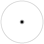
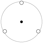
blah

spacer pentagon

trigonal bipyramid

spacer square pyramid

spacer octahedron

spacer trigonal prism

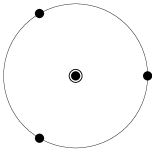
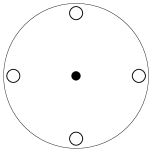
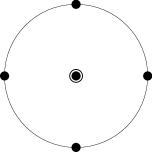
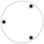
blah

spacer hexagon

pentagonal bipyramid

capped trigonal antiprism

spacer cube

square antiprism

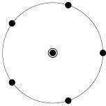
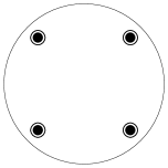
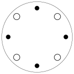
blah

spacer hexagonal bipyramid

spacer augmented trigonal prism

spacer capped square prism

spacer capped square antiprism

bicapped square antiprism

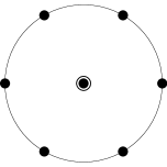
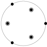
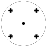
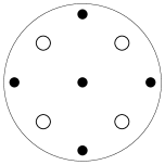
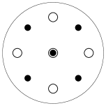
blah

icosahedron

cuboctahedron

dodecahedron

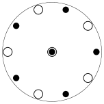
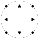
Table 1: Candidate crystal structures with $P$ plane waves, specified by their symmetry group $\mathcal{G}$ and Föppl configuration. Bars denote dimensionless equivalents: $\bar{\beta}=\beta\,{\delta\mu}^{2}$, $\bar{\gamma}=\gamma\,{\delta\mu}^{4}$, $\bar{\Omega}=\Omega/({\delta\mu}_{2}^{2}N_{0})$ with $N_{0}=2\bar{\mu}^{2}/\pi^{2}$. $\bar{\Omega}_{\min}$ is the (dimensionless) minimum free energy at ${\delta\mu}={\delta\mu}_{2}$, obtained from (3.36). The phase transition (first order for $\bar{\beta}<0$ and $\bar{\gamma}>0$, second order for $\bar{\beta}>0$ and $\bar{\gamma}>0$) occurs at ${\delta\mu}_{*}$.

	Structure	P	$\mathcal{G}$(Föppl)	$\bar{\beta}$	$\bar{\gamma}$	$\bar{\Omega}_{\min}$	${\delta\mu}_{*}/\Delta_{0}$
1	point	1	$C_{\infty v}$(1)	0.569	1.637	0	0.754
2	antipodal pair	2	$D_{\infty v}$(11)	0.138	1.952	0	0.754
3	triangle	3	$D_{3h}$(3)	-1.976	1.687	-0.452	0.872
4	tetrahedron	4	$T_{d}$(13)	-5.727	4.350	-1.655	1.074
5	square	4	$D_{4h}$(4)	-10.350	-1.538	–	–
6	pentagon	5	$D_{5h}$(5)	-13.004	8.386	-5.211	1.607
7	trigonal bipyramid	5	$D_{3h}$(131)	-11.613	13.913	-1.348	1.085
8	square pyramid	5	$C_{4v}$(14)	-22.014	-70.442	–	–
9	octahedron	6	$O_{h}$(141)	-31.466	19.711	-13.365	3.625
10	trigonal prism	6	$D_{3h}$(33)	-35.018	-35.202	–	–
11	hexagon	6	$D_{6h}$(6)	23.669	6009.225	0	0.754
12	pentagonal	7	$D_{5h}$(151)	-29.158	54.822	-1.375	1.143
	bipyramid
13	capped trigonal	7	$C_{3v}$($13\bar{3}$)	-65.112	-195.592	–	–
	antiprism
14	cube	8	$O_{h}$(44)	-110.757	-459.242	–	–
15	square antiprism	8	$D_{4d}$($4\bar{4}$)	-57.363	-6.866	–	–
16	hexagonal	8	$D_{6h}$(161)	-8.074	5595.528	$-2.8\times 10^{-6}$	0.755
	bipyramid
17	augmented	9	$D_{3h}$($3\bar{3}\bar{3}$)	-69.857	129.259	-3.401	1.656
	trigonal prism
18	capped	9	$C_{4v}$(144)	-95.529	7771.152	-0.0024	0.773
	square prism
19	capped	9	$C_{4v}$($14\bar{4}$)	-68.025	106.362	-4.637	1.867
	square antiprism
20	bicapped	10	$D_{4d}$($14\bar{4}1$)	-14.298	7318.885	$-9.1\times 10^{-6}$	0.755
	square antiprism
21	icosahedron	12	$I_{h}$($15\bar{5}1$)	204.873	145076.754	0	0.754
22	cuboctahedron	12	$O_{h}$($4\bar{4}\bar{4}$)	-5.296	97086.514	$-2.6\times 10^{-9}$	0.754
23	dodecahedron	20	$I_{h}$(5555)	-527.357	114166.566	-0.0019	0.772

Because the LOFF pairing rings have an opening angle $\psi_{0}\simeq 67.1^{\circ}$, no more than nine rings can be arranged on the Fermi surface without any intersection [33, 34]. For this reason we have focussed on crystal structures with nine or fewer waves, but we have included several structures with more waves in order to verify that such structures are not favored. We have tried to analyze a fairly exhaustive list of candidate structures. All five Platonic solids are included in Table 1, as is the simplest Archimedean solid, the cuboctahedron. (All other Archimedean solids have even more vertices.) We have analyzed many dihedral polyhedra and polygons: regular polygons, bipyramids, prisms, antiprisms, and various capped or augmented polyhedra. For each crystal structure we list the crystal point group $\mathcal{G}$ and the Föppl configuration of the polyhedron or polygon. The Föppl configuration is a list of the number of vertices on circles formed by intersections of the sphere with consecutive planes perpendicular to the principal symmetry axis of the polyhedron or polygon. We use a modified notation where $a$ or $\bar{a}$ indicates that the points on a given circle are respectively eclipsed or staggered relative to the circle above. Note that polyhedra with several different principal symmetry axes, namely those with $T$, $O$, or $I$ symmetry, have several different Föppl descriptions: for example, a cube is $(44)$ along a fourfold symmetry axis or $(13\bar{3}1)$ along a threefold symmetry axis. (That is, the cube can equally be described as a square prism or a bicapped trigonal antiprism. This should make clear that the singly capped trigonal antiprism of Fig. 10 and Table 1 is a cube with one vertex removed.)

We do not claim to have analyzed all possible crystal structures, since that is an infinite task. However, there are several classic mathematical problems regarding extremal arrangements of points on a sphere and, although we do not know that our problem is related to one of these, we have made sure to include solutions to these problems. For example, many of the structures that we have evaluated correspond to solutions of Thomson’s problem [39, 33] (lowest energy arrangement of $P$ point charges on the surface of a sphere) or Tammes’s problem [34, 33] (best packing of $P$ equal circles on the surface of a sphere without any overlap). In fact, we include all solutions to the Thomson and Tammes problems for $P\leq 9$. Our list also includes all “balanced” configurations [40] that are possible for nonintersecting rings: a balanced configuration is a set $\mathcal{Q}$ with a rotational symmetry about every ${\mathbf{q}}\in\mathcal{Q}$; this corresponds to an arrangement of particles on a sphere for which the particles are in equilibrium for any two-particle force law.

For each crystal structure, we have calculated the quartic and sextic coefficients $\beta$ and $\gamma$ according to Eqs. (3.30), using methods described in the appendix to calculate all the $J$ and $K$ integrals. To further discriminate among the various candidate structures, we also list the minimum free energy $\Omega_{\min}$ evaluated at the plane-wave instability point ${\delta\mu}={\delta\mu}_{2}$ where $\alpha=0$. To set the scale, note that the BCS state at ${\delta\mu}=0$ has $\Omega_{\rm BCS}=-\mu^{2}\Delta_{0}^{2}/\pi^{2}$, corresponding to $\bar{\Omega}_{\rm BCS}=-0.879$ in the units of Table 1. For those configurations with $\beta>0$ and $\gamma>0$, $\Omega_{\min}=0$ at ${\delta\mu}={\delta\mu}_{2}$ and $\Omega_{\min}<0$ for ${\delta\mu}<{\delta\mu}_{2}$, where $\alpha<0$. Thus, we find a second-order phase transition at ${\delta\mu}={\delta\mu}_{2}$. For those configurations with $\beta<0$ and $\gamma>0$, at ${\delta\mu}={\delta\mu}_{2}$ the minimum free energy occurs at a nonzero $\Delta$ with $\Omega_{\min}<0$. (The value of $\Delta$ at which this minimum occurs can be obtained from (3.36).) Because $\Omega_{\min}<0$ at ${\delta\mu}={\delta\mu}_{2}$, if we go to ${\delta\mu}>{\delta\mu}_{2}$, where $\alpha>0$, we lift this minimum until at some ${\delta\mu}_{*}$ it has $\Omega=0$ and becomes degenerate with the $\Delta=0$ minimum. At ${\delta\mu}={\delta\mu}_{*}$, a first-order phase transition occurs. For a very weak first-order phase transition, ${\delta\mu}_{*}\simeq{\delta\mu}_{2}\simeq 0.754\Delta_{0}$. For a strong first-order phase transition, ${\delta\mu}_{*}\gg{\delta\mu}_{2}$ and the crystalline color superconducting phase prevails as the favored ground state over a wider range of ${\delta\mu}$.

3.5 Crystal structures with intersecting rings lose

There are seven configurations in Table 1 with very large positive values for $\gamma$. These are precisely the seven configurations that have intersecting pairing rings: the hexagon, hexagonal prism, capped square prism, bicapped square antiprism, icosahedron, cuboctahedron, and dodecahedron. The first two of these include hexagons, and since $\psi_{0}>60^{\circ}$ the rings intersect. The last four of these crystal structures have more than nine rings, meaning that intersections between rings are also inevitable. The capped square prism is an example of a nine-wave structure with intersecting rings. It has a $\gamma$ which is almost two orders of magnitude larger than that of the augmented trigonal prism and the capped square antiprism which, in contrast, are nine wave structures with no intersecting rings. Because of their very large $\gamma$’s all the structures with intersecting rings have either second-order phase transitions or very weak first-order phase transitions occurring at a ${\delta\mu}_{*}\simeq{\delta\mu}_{2}$. At ${\delta\mu}={\delta\mu}_{2}$, all these crystal structures have $\Omega_{\min}$ very close to zero. Thus, as our analysis of two plane waves led us to expect, we conclude that these crowded configurations with intersecting rings are disfavored.

3.6 “Regular” crystal structures rule, and the cube rules them all

At the opposite extreme, we see that there are several structures that have negative values of $\gamma$: the square, square pyramid, square antiprism, trigonal prism, capped trigonal antiprism, and cube. Our analysis demonstrates that the transition to all these crystal structures (as to those with $\beta<0$ and $\gamma>0$) is first order. But, we cannot evaluate $\Omega_{\min}$ or ${\delta\mu}_{*}$ because, to the order we are working, $\Omega$ is unbounded from below. For each of these crystal structures, we could formulate a well-posed (but difficult) variational problem in which we make a variational ansatz corresponding to the structure, vary, and find $\Omega_{\min}$ without making a Ginzburg-Landau approximation. It is likely, therefore, that within the Ginzburg-Landau approximation $\Omega$ will be stabilized at a higher order than the sextic order to which we have worked.

Of the sixteen crystal structures with no intersecting rings, there are seven that are particularly favored by the combinatorics of Eqs. (3.30). It turns out that these seven crystal structures are precisely the six that we have found with $\gamma<0$, plus the octahedron, which is the most favored crystal structure among those with $\gamma>0$. As discussed earlier, more terms contribute to the rhombic and hexagonal sums in Eqs. (3.30) when the ${\mathbf{q}}$’s are arranged in such away that their vertices form rectangles, trapezoids, and cuboids inscribed in the sphere $|{\mathbf{q}}|=q_{0}$. Thus the square itself fares well, as do the square pyramid, square antiprism, and trigonal prism which contain one, two, and three rectangular faces, respectively. The octahedron has three square cross sections. However, the cube is the outstanding winner because it has six rectangular faces, six rectangular cross sections, and also allows the five-corner arrangements described previously. The capped trigonal antiprism in Table 1 is a cube with one vertex removed. This seven-wave crystal has almost as many waves as the cube, and almost as many combinatorial advantages as the cube, and it turns out to have the second most negative $\gamma$.

With eight rings, the cube is close to the maximum packing for nonintersecting rings with opening angle $\psi_{0}\simeq 67.1^{\circ}$. Although nine rings of this size can be packed on the sphere, adding a ninth ring to the cube and deforming the eight rings into a cuboid, as we have done with the capped square prism, necessarily results in intersecting rings and the ensuing cost overwhelms the benefits of the cuboidal structure. To form a nine-ring structure with no intersections requires rearranging the eight rings, spoiling the favorable regularities of the cuboid. Therefore a nine-ring arrangement is actually less favorable than the cuboid, even though it allows one more plane wave. We see from Table 1 that $\gamma$ for the cube is much more negative than that for any of the other combinatorially favored structures. The cube is our winner, and we understand why.

To explore the extent to which the cube is favored, we can compare it to the octahedron, which is the crystal structure with $\gamma>0$ for which we found the strongest first-order phase transition, with the largest ${\delta\mu}_{*}$ and the deepest $\Omega_{\min}$. The order $\Delta^{6}$ free energy we have calculated for the cube is far below that for the octahedron at all values of $\Delta$. To take an extreme example, at ${\delta\mu}={\delta\mu}_{2}$ the octahedron has $\bar{\Omega}_{\min}=-13.365$ at $\Delta=1.263{\delta\mu}_{2}=0.953\Delta_{0}$ whereas for the cube we find that $\bar{\Omega}=-2151.5$ at this $\Delta$. As another example, suppose that we arbitrarily add $+{\textstyle\frac{1}{4}}800\Delta^{8}/{\delta\mu}^{8}$ to the $\bar{\Omega}$ of the cube. In this case, at ${\delta\mu}={\delta\mu}_{2}$ we find that the cube has $\bar{\Omega}_{\min}=-32.5$ at $\Delta=0.656\Delta_{0}$ and is thus still favored over the octahedron, even though we have not added any $\Delta^{8}$ term to the free energy of the octahedron. These numerical exercises demonstrate the extraordinary robustness of the cube, but should not be taken as more than qualitative. We do not know at what $\Delta$ and at what value $\Omega_{\min}$ the true free energy for the cube finds its minimum. However, because the qualitative features of the cube are so favorable we expect that it will have a deeper $\Omega_{\min}$ and a larger ${\delta\mu}_{*}$ than the octahedron. Within the Ginzburg-Landau approximation, the octahedron already has $\Delta=0.953\Delta_{0}$ and a deep $\bar{\Omega}_{\min}=-13.365$, about fifteen times deeper than $\bar{\Omega}_{\rm BCS}=-0.879$ for the BCS state at ${\delta\mu}=0$.

Even if we were to push the Ginzburg-Landau analysis of the cube to higher order and find a stable $\Omega_{\min}$, we would not be able to trust such a result quantitatively. Because it predicts a strong first-order phase transition, the Ginzburg-Landau approximation predicts its own quantitative demise. What we have learned from it, however, is that there are qualitative reasons that make the cube the most favored crystal structure of them all. And, to the extent that we can trust the quantitative calculations qualitatively, they indicate that the first-order phase transition results in a state with $\Delta$ comparable to or bigger than that in the BCS phase, with $\Omega_{\min}$ comparable to or deeper than that of the BCS phase, and occurs at a ${\delta\mu}_{*}\gg{\delta\mu}_{2}$.

3.7 Varying continuous degrees of freedom

None of the regularities of the cube which make it so favorable are lost if it is deformed continuously into a cuboid, slightly shorter or taller than it is wide, as long as it is not deformed so much as to cause rings to cross. Next, we investigate this and some of the other possible continuous degrees of freedom present in a number of the crystal structures we have described above.

So far we have neglected the fact, mentioned at the start of this section, that some of the candidate structures have multiple orbits under the action of the point group $\mathcal{G}$. These structures include the square pyramid, the four bipyramids, and the five capped or augmented structures listed in Table 1; all have two orbits except for the three singly capped crystal structures, which have three orbits. For these multiple-orbit structures each orbit should have a different gap parameter but in Table 1 we have assumed that all the gaps are equal. We have, however, analyzed each of these structures upon assuming different gaps, searching for a minimum of the free energy in the two- or three-dimensional parameter space of gaps. In most cases, the deepest minimum is actually obtained by simply eliminating one of the orbits from the configuration (i.e. let $\Delta=0$ for that orbit); the resultant structure with one less orbit appears as another structure in Table 1. For example, the bicapped square antiprism has two orbits: the first is the set of eight ${\mathbf{q}}$’s forming a square antiprism, the second is the antipodal pair of ${\mathbf{q}}$’s forming the two “caps” of the structure. Denote the gaps corresponding to these two orbits as $\Delta_{1}$ and $\Delta_{2}$. This structure is overcrowded with intersecting rings, so it is not surprising to find that a lower-energy configuration is obtained by simply letting $\Delta_{2}=0$, which gives the “uncapped” square antiprism. Configurations with fewer orbits are generally more favorable, with only three exceptions known to us: the trigonal bipyramid is favored over the triangle or the antipodal pair; the square pyramid is favored over the square or the point; and the capped trigonal antiprism is favored over any of the structures that can be obtained from it by removing one or two orbits. For these configurations, Table 1 lists the results for $\Delta_{1}=\Delta_{2}\,(=\Delta_{3})$; the numbers can be slightly improved with $\Delta_{1}\neq\Delta_{2}\,(\neq\Delta_{3})$ but the difference is unimportant.

For some configurations in Table 1 the positions of the points are completely fixed by symmetry while for others the positions of the points can be varied continuously, while still maintaining the point-group symmetry of the structure. For example, with the square pyramid we can vary the latitude of the plane that contains the inscribed pyramid base. Similarly, with the various polygonal prism and antiprism structures (and associated cappings and augmentations), we can vary the latitudes of the inscribed polygons (equivalently, we can vary the heights of these structures along the principal symmetry axis). For each structure that has such degrees of freedom, we have scanned the allowed continuous parameter space to find the favored configuration. Table 1 then shows the results for this favored configuration, and the latitude angles describing the favored configuration are given as footnotes. However, if the structure always has overlapping rings regardless of its deformation, then either no favorite configuration exists or the favorite configuration is a degenerate one that removes the overlaps by changing the structure. There are two instances where this occurs: the capped square prism can be deformed into a square pyramid by shrinking the height of the square prism to zero, and the bicapped square antiprism can be deformed into an antipodal pair by moving the top and bottom square faces of the antiprism to the north and south poles, respectively. For these structures, Table 1 just lists results for an arbitrarily chosen nondegenerate configuration.

\psfrag{x1}[tc][tc]{\small$10^{\circ}$}\psfrag{x2}[tc][tc]{\small$20^{\circ}$}\psfrag{x3}[tc][tc]{\small$30^{\circ}$}\psfrag{x4}[tc][tc]{\small$40^{\circ}$}\psfrag{x5}[tc][tc]{\small$50^{\circ}$}\psfrag{x6}[tc][tc]{\small$60^{\circ}$}\psfrag{x7}[tc][tc]{\small$70^{\circ}$}\psfrag{x8}[tc][tc]{\small$80^{\circ}$}\psfrag{x9}[tc][tc]{\small$90^{\circ}$}\psfrag{x10}[tc][tc]{\small$50^{\circ}$}\psfrag{x11}[tc][tc]{\small$55^{\circ}$}\psfrag{x12}[tc][tc]{\small$60^{\circ}$}\psfrag{x13}[tc][tc]{\small$65^{\circ}$}\psfrag{y1}[rc][rc]{\small 3000}\psfrag{y2}[rc][rc]{\small 6000}\psfrag{y3}[rc][rc]{\small 9000}\psfrag{y4}[rc][rc]{\small 12000}\psfrag{y5}[rc][rc]{\small 15000}\psfrag{y6}[rc][rc]{\small 30}\psfrag{y7}[rc][rc]{\small 60}\psfrag{y8}[rc][rc]{\small 90}\psfrag{y9}[rc][rc]{\small 120}\psfrag{y10}[rc][rc]{\small 150}\psfrag{xlabel}{$\theta$}\psfrag{ylabel}{$\gamma(\theta){\delta\mu}^{4}$}\includegraphics[width=433.62pt]{squareantiprismplot.eps}

Figure 11: The sextic free energy coefficient $\gamma$ for the square antiprism as a function of the polar (latitude) angle $\theta$ of the top square facet. (The polar angle of the bottom square facet is $\pi-\theta$.) The inset plot shows the detail in the range of $\theta$ where no rings intersect. Solid and dashed vertical lines indicate the positions of primary and secondary singularies as discussed in the text (other secondary singularities occur, but are not discernible on the plot).

A typical parameter scan is shown in Fig, 11, where we have plotted $\gamma$ for the square antiprism as a function of the polar angle $\theta$ of the top square facet (the polar angle of the bottom square facet is $\pi-\theta$). As we expect, $\gamma$ is very large in regions where any rings intersect, and we search for a minimum of $\gamma$ in the region where no rings intersect. The plot has a rather complicated structure of singularities and discontinuities; these features are analogous to those of Fig. 9, and as there they arise as a result of the double limit we are taking. Primary singularities occur at critical angles where pairing rings are mutually tangent on the Fermi surface. Secondary singularities occur where rings corresponding to harmonic ${\mathbf{q}}$’s, obtained by taking sums and differences of the fundamental ${\mathbf{q}}$’s that define the crystal structure, are mutually tangent. Such ${\mathbf{q}}$’s arise in the calculation of $J$ and $K$ because these calculations involve momenta corresponding to various diagonals of the rhombus and hexagon in Fig. 7.

In addition to varying the latitudes of the Föppl planes in various structures, we varied “twist angles”. For example, we explored the continuous degree of freedom that turns a cube into a square antiprism, by twisting the top square relative to the bottom square by an angle $\phi$ ranging from $0^{\circ}$ to $45^{\circ}$. In Fig. 12, we show a parameter scan in which we simultaneously vary the twist angle $\phi$ and the latitudes of the square planes in such a way that the scan interpolates linearly from the cube to the most favorable square antiprism of Table 1. In this parameter scan, we find a collection of secondary singularities and one striking fact: $\gamma$ is much more negative when the twist angle is zero (i.e. for the cube itself) than for any nonzero value. For the cube, $\gamma=-459.2/{\delta\mu}^{4}$, whereas the best one can do with a nonzero twist is $\gamma=-64.2/{\delta\mu}^{4}$, which is the result for an infinitesimal twist angle. Thus, any nonzero twist spoils the regularities of the cube that contribute to its combinatorial advantage, and this has a dramatic and unfavorable effect on the free energy.

\psfrag{5}[tc][tc]{\small$5^{\circ}$}\psfrag{10}[tc][tc]{\small$10^{\circ}$}\psfrag{15}[tc][tc]{\small$15^{\circ}$}\psfrag{20}[tc][tc]{\small$20^{\circ}$}\psfrag{25}[tc][tc]{\small$25^{\circ}$}\psfrag{30}[tc][tc]{\small$30^{\circ}$}\psfrag{35}[tc][tc]{\small$35^{\circ}$}\psfrag{40}[tc][tc]{\small$40^{\circ}$}\psfrag{45}[tc][tc]{\small$45^{\circ}$}\psfrag{-500}[rc][rc]{\small-500}\psfrag{-400}[rc][rc]{\small-400}\psfrag{-300}[rc][rc]{\small-300}\psfrag{-200}[rc][rc]{\small-200}\psfrag{-100}[rc][rc]{\small-100}\psfrag{-100}[rc][rc]{\small-100}\psfrag{100}[rc][rc]{\small 100}\psfrag{200}[rc][rc]{\small 200}\psfrag{xlabel}{$\phi$}\psfrag{ylabel}{$\gamma(\phi){\delta\mu}^{4}$}\psfrag{arrowlabel1}[lb][lt]{cube}\psfrag{arrowlabel2}[tc][rb]{\mbox{square antiprism}}\includegraphics[width=361.34999pt]{twistfig.eps}

Figure 12: The sextic free energy coefficient $\gamma$ for a scan that linearly interpolates from the cube (twist angle $\phi=0$) to the square antiprism of Table 1 (twist angle $\phi=45^{\circ}$). Dashed vertical lines indicate secondary singularities.

Finally, we have scanned the parameter space of a generic cuboid to see how this compares to the special case of a cube. That is, we vary the height of the cuboid relative to its width, without introducing any twist. This continuous variation does not reduce the combinatorial advantage of the crystal structure. As expected, therefore, we find that as long as the cuboid has no intersecting rings, it has a free energy that is very similar to that of the cube itself. Any cuboid with intersecting rings is very unfavorable. In the restricted parameter space of nonintersecting cuboidal arrangements, the cuboid with the most negative free energy is a square prism with a polar angle of $51.4^{\circ}$ for the top square face. (For this polar angle the pairing rings corresponding to the four corners of the square are almost mutually tangent.) This prism is slightly taller than a perfect cube, which has a polar angle of $54.7^{\circ}$. The free energy coefficients of the best cuboid are $\beta=-111.563/({\delta\mu})^{2}$, $\gamma=-463.878/({\delta\mu})^{4}$. These coefficients differ by less than $1\%$ from those for the cube, given in Table 1. There is no significant difference between the cube and this very slightly more favorable cuboid: all the qualitative arguments that favor the cube favor any cuboid with no intersecting rings equally well. We therefore expect that if we could determine the exact (rather than Ginzburg-Landau) free energy, we would find that the favored crystal structure is a cuboid with a polar angle somewhere between $51.4^{\circ}$ and $56.5^{\circ}$, as this is the range for which no rings intersect. We expect no important distinction between the free energy of whichever cuboid in this narrow range happens to be favored and that of the cube itself.

4 Conclusions and Open Questions

We have argued that the cube crystal structure is the favored ground state at zero temperature near the plane-wave instability point ${\delta\mu}={\delta\mu}_{2}$. By the cube we mean a crystal structure constructed as the sum of eight plane waves with wave vectors pointing towards the corners of a cube. The qualitative points (which we have demonstrated in explicit detail via the analysis of many different crystal structures) that lead us to conclude that the cube is the winner are:

• The quadratic term in the Ginzburg-Landau free energy wants a $|{\mathbf{q}}|$ such that the pairing associated with any single choice of $\hat{\mathbf{q}}$ occurs on a ring with opening angle $\psi_{0}\simeq 67.1^{\circ}$ on each Fermi surface.

• The quadratic term in the Ginzburg-Landau free energy favors condensation with many different wave vectors, and thus many different pairing rings on the Fermi surfaces. However, the quartic and sextic terms in the free energy strenuously prohibit the intersection of pairing rings. No more than nine rings with opening angle $67.1^{\circ}$ can be placed on the sphere without overlap.

• The quartic and sextic terms favor regular crystal structures, for example those that include many different sets of wave vectors whose tips form rectangles. None of the nine-wave structures with no intersections between pairing rings are regular in the required sense. The cube is a very regular eight-wave crystal structure.

Quantitatively, we find that a cube (actually, a cuboid that is only slightly taller than it is wide) has by far the most negative Ginzburg-Landau free energy, to sextic order, of all the many crystal structures we have investigated.

\psfrag{0}{\small 0}\psfrag{0.25}{\small 0.25}\psfrag{0.5}{\small 0.5}\psfrag{0.75}{\small 0.75}\psfrag{1}{\small 1}\includegraphics{unitcell.eps}

Figure 13: A unit cell of the LOFF face-centered-cubic crystal. The gray planes are surfaces where $\Delta({\mathbf{x}})=0$. The darker surfaces are contours where $\Delta({\mathbf{x}})=+4\Delta$, and the lighter surfaces are contours where $\Delta({\mathbf{x}})=-4\Delta$.

Let us now see what the cubic crystal structure looks like in position space. The eight ${\mathbf{q}}$ vectors are the eight shortest vectors in the reciprocal lattice of a face-centered-cubic crystal. Therefore, we find that $\Delta({\mathbf{x}})$ exhibits face-centered-cubic symmetry. Explicitly,

$$\Delta({\mathbf{x}}) = 2\Delta\Biggl{[}\cos\frac{2\pi}{a}(x+y+z)+\cos\frac{2\pi}{a}(x-y+z)$$ (4.41)

$$+\cos\frac{2\pi}{a}(x+y-z)+\cos\frac{2\pi}{a}(-x+y+z)\Biggr{]}\ ,$$

where the lattice constant (i.e. the edge length of the unit cube) is

$$a=\frac{\sqrt{3}\pi}{|{\mathbf{q}}|}\simeq\frac{4.536}{{\delta\mu}}\simeq\frac{6.012}{\Delta_{0}}\ ,$$ (4.42)

where the last equality is valid at ${\delta\mu}={\delta\mu}_{2}$ and where $\Delta_{0}$ is the gap of the BCS phase that would occur at ${\delta\mu}=0$. A unit cell of the crystal is shown in Fig. 13. We have taken $\Delta({\mathbf{x}})$ to be real by convention: we have the freedom to multiply $\Delta({\mathbf{x}})$ by an overall ${\mathbf{x}}$-independent phase. This freedom corresponds to the fact that the condensate spontaneously breaks the $U(1)$ symmetry associated with conservation of quark number.

Our Ginzburg-Landau analysis predicts a first-order phase transition to the cubic crystalline color superconductor at some ${\delta\mu}={\delta\mu}_{*}$. The fact that we predict a first-order phase transition means that the Ginzburg-Landau analysis cannot be trusted quantitatively. Furthermore, at order $\Delta^{6}$, which is as far as we have gone, the Ginzburg-Landau free energy for the cube is unbounded from below. We therefore have no quantitative prediction of ${\delta\mu}_{*}$ or the magnitude of $\Delta$. The best we can do is to note that the cube is significantly favored over the octahedron, for which the order $\Delta^{6}$ Ginzburg-Landau analysis predicts ${\delta\mu}_{*}\simeq 3.6\Delta_{0}$ and predicts that at ${\delta\mu}={\delta\mu}_{2}=0.754\Delta_{0}$, the gap is $\Delta\simeq 0.95\Delta_{0}$ and the condensation energy is larger than that in the BCS state by a factor of about fifteen. As we have warned repeatedly, these numbers should not be trusted quantitatively: because the Ginzburg-Landau approximation predicts a strong first-order phase transition, it predicts its own breakdown. We have learned several qualitative lessons from it, however:

• We have understood the qualitative reasons that make the cube the most favored crystal structure of them all.

• The Ginzburg-Landau analysis indicates that $\Delta$, the gap parameter in the crystalline phase, is comparable to $\Delta_{0}$, that in the BCS phase.

• We learn that the condensation energy by which the crystalline phase is favored over unpaired quark matter at ${\delta\mu}\neq 0$ may even be larger than that for the BCS phase at ${\delta\mu}=0$. (Note that the spatial average of $\Delta({\mathbf{x}})^{2}$ in (4.41) is $8\Delta^{2}$. It is not surprising that $\Delta\sim\Delta_{0}$ corresponds to an $|\Omega_{\min}|$ in the crystalline phase which is larger than $|\Omega_{\rm BCS}|$.)

• We learn that the crystalline color superconductivity window ${\delta\mu}_{1}<{\delta\mu}<{\delta\mu}_{*}$ is large. Because ${\delta\mu}_{2}$ is not much larger than ${\delta\mu}_{1}$, the window ${\delta\mu}_{1}<{\delta\mu}<{\delta\mu}_{2}$ wherein the single plane-wave condensate is possible is narrow. We have learned, however, that ${\delta\mu}_{*}\gg{\delta\mu}_{2}$. Furthermore, because the condensation energy of the crystalline phase is so robust, much greater than that for the single plane wave and likely comparable to that for the BCS phase, the value of ${\delta\mu}_{1}$, the location of the transition between the crystalline phase and the BCS phase, will be significantly depressed.

Much remains to be done:

• Our Ginzburg-Landau analysis provides a compelling argument that the crystalline color superconductor is face-centered-cubic. Given that, and given the prediction of a strong first-order phase transition, the Ginzburg-Landau approximation should now be discarded. What should be taken from our work is the prediction that the structure (4.41) is favored. Although $\Delta$ could be estimated by going to higher order in the Ginzburg-Landau approximation, a much better strategy is to do the calculation of $\Delta$ upon assuming the crystal structure (4.41) but without requiring $\Delta$ to be small. One possible method of analysis, along the lines of that applied in Refs. [22, 27, 15] to the single plane wave, would be to find a variational wave function that incorporates the structure (4.41), vary within this ansatz, and find $\Delta$ and $\Omega_{\min}$. Another possibility is to assume (4.41) and then truncate the infinite set of coupled Nambu-Gorkov gap equations without assuming $\Delta$ is small. This strategy would be the analogue of that applied to the chiral crystal in Ref. [31]. A third possibility is to analyze the state with crystal structure (4.41) using methods like those applied to the two plane-wave (antipodal pair) crystal structure in Ref. [41]. Regardless of what method is used, because $\Delta\neq 0$ a complete calculation would require the inclusion of condensates with ${\mathbf{q}}$’s corresponding to higher harmonics of the fundamental ${\mathbf{q}}$’s that define the crystal structure.

• The cubic crystal structure (4.41) breaks $x$-, $y$- and $z$-translational invariance, and therefore has three phonon modes. With the crystal structure (4.41) in hand, it would be very interesting to use the methods developed in Refs. [17] to derive the dispersion relations for these phonons and compute the parameters of the low energy effective Lagrangian describing these phonons.

• How could the “crystalline superfluid” state be detected in an ultracold gas of fermionic atoms? The simplest idea would be to look for the periodic modulation of the atom density, which goes like $\Delta(x)^{2}\mu^{2}$. This means that the ratio of the magnitude of the spatial modulation of the density to the density itself is of order $\Delta(x)^{2}/\mu^{2}$. Since the density modulation is only sensitive to $\Delta(x)^{2}$, it will not see the sign of $\Delta$ in Fig. 13. That is, the crystal structure for $\Delta^{2}$ is simple cubic, with a unit cell of size $a/2$.

• In the QCD context, we need to do a three-flavor analysis, beginning with the unpaired quark matter of (1.2) and letting $ud$, $us$ and $us$ crystalline condensates form. Given the robustness of the crystalline color superconducting condensates we have found, we expect the three-flavor crystalline color superconductor gap, critical temperature and condensation energy to be comparable to or even larger than those of the CFL phase. This means that just as the crystalline color superconductor will push ${\delta\mu}_{1}$ down in our model, in three flavor QCD it will push the unlocking transition between the CFL and crystalline phases up to a higher density than has been estimated to date, since present estimates have assumed the condensation energy in the crystalline phase is negligible. It also means that just as in our model the crystalline window ${\delta\mu}_{1}<{\delta\mu}<{\delta\mu}_{*}$ is in no sense narrow, crystalline color superconductivity will be a generic feature of nature’s QCD phase diagram, occurring wherever quark matter that is not color-flavor locked is to be found.

• What effects could the presence of a layer of crystalline color superconducting quark matter have on observable properties of a compact star? Could it be the place where some pulsar glitches originate, as suggested in Ref. [15]? The next step toward answering this question and toward studying the properties of glitches that may originate within crystalline color superconducting quark matter is to take the crystal structure (4.41) and rotate it. What is the structure of a rotational vortex in this phase? Are vortices pinned? It is reasonable to guess that the vortex core will prefer to live where the condensate is already weakest, thus along the line of intersection of two of the nodal planes in Fig. 13. If this intuition is correct, the vortices would be pinned. Constructing the vortices explicitly (and then calculating the pinning force) will be a challenge. Vortices are usually constructed beginning with a Ginzburg-Landau free energy functional written in terms of $\Delta({\mathbf{x}})$ and $\nabla\Delta({\mathbf{x}})$. Instead, we have constructed a Ginzburg-Landau functional written in terms of the $\Delta_{\mathbf{q}}$’s. In principle, this contains the same information. But, it is not well-suited to the analysis of a localized object like a vortex. This means that it will take some thought to come up with a sensible model within which one can construct a vortex in the crystalline condensate (4.41).

  The greatest difficulties in finding the explicit form of a vortex will be in determining the details of how the vortex core interacts with the crystal structure. Unfortunately, therefore, calculating the pinning force will likely be a hard problem. As always, it should be easier to understand the physics of a vortex far from its core. The natural expectation is that far from its core, a vortex will be described simply by multiplying the $\Delta({\mathbf{x}})$ of (4.41) by $\exp[i\theta({\mathbf{x}})]$, where $\theta({\mathbf{x}})$ is a slowly varying function of ${\mathbf{x}}$ that winds once from 0 to $2\pi$ as you follow a loop encircling the vortex at a large distance. In a uniform superfluid, this slowly varying phase describes a particle-number current flowing around the vortex. Here, the nodal planes make this interpretation difficult. Thus, even the long distance vortex physics will be interesting to work out.

• Our analysis does not apply to QCD at asymptotically high density, where the QCD coupling becomes weak. In this regime, quark-quark scattering is dominated by gluon exchange and because the gluon propagator is almost unscreened, the scattering is dominated by forward scattering. This works in favor of crystalline color superconductivity [18], but it also has the consequence of reducing $q_{0}/{\delta\mu}$ and hence reducing $\psi_{0}$. The authors of Ref. [18] find $q_{0}/{\delta\mu}$ reduced almost to 1, meaning $\psi_{0}$ reduced almost to zero. However, the authors of Ref. [20] find $q_{0}/{\delta\mu}\simeq 1.16$ at asymptotically high density, meaning that $\psi_{0}\simeq 61^{\circ}$. If the opening angle of the pairing rings on the Fermi surface does become very small at asymptotic densities, then the crystal structure there is certain to be qualitatively different from that which we have found. At present, the crystal structure at asymptotic densities is unresolved. This is worth pursuing, since it should ultimately be possible to begin with asymptotically free QCD (rather than a model thereof) and calculate the crystal structure at asymptotic density from first principles. (At these densities, the strange quark mass is irrelevant and a suitable ${\delta\mu}$ would have to be introduced by hand.) Although such a first-principles analysis of the crystalline color superconducting state has a certain appeal, it should be noted that the asymptotic analysis of the CFL state seems to be quantitatively reliable only at densities that are more than fifteen orders of magnitude larger than those reached in compact stars [42]. At accessible densities, models like the one we have employed are at least as likely to be a good starting point.

Acknowledgements

We are grateful to Mark Alford, Joydip Kundu, Vincent Liu, Eugene Shuster, Dam Son and Frank Wilczek for helpful discussions and to Liev Aleo for editorial assistance. We are grateful for the support and hospitality of the Institute for Theoretical Physics at Santa Barbara, in the case of JAB via the ITP Graduate Fellows program. This research was supported in part by the U.S. Department of Energy (D.O.E.) under cooperative research agreement #DF-FC02-94ER40818, and by the National Science Foundation under Grant No. PHY99-07949. The work of JAB was supported in part by a DOD National Defense Science and Engineering Graduate Fellowship.

Appendix

In this Appendix, we outline the explicit evaluation of the loop integrals in Eqs. (2.2) that occur in $\Pi$, $J$ and $K$. For all loop integrals, the momentum integration is restricted to modes near the Fermi surface by a cutoff $\omega\ll\bar{\mu}$, meaning that the density of states can be taken as constant within the integration region:

$$\int d^{4}p=\int_{-\infty}^{+\infty}dp^{0}\int_{\bar{\mu}-\omega}^{\bar{\mu}+\omega}|{\mathbf{p}}|^{2}d|{\mathbf{p}}|\int_{4\pi}d\hat{{\mathbf{p}}}\approx\bar{\mu}^{2}\int_{-\infty}^{+\infty}dp^{0}\int_{-\omega}^{+\omega}ds\int_{4\pi}d\hat{{\mathbf{p}}}$$ (A.1)

where $s\equiv|{\mathbf{p}}|-\bar{\mu}$. Each integral is further simplified by removing the antiparticle poles from the bare propagators $G^{(0)}$ and $\bar{G}^{(0)}$ that appear in the integrand. (We can disregard the antiparticles because their effect on the Fermi surface physics of interest is suppressed by of order $\Delta/\bar{\mu}$.) To see how to remove the antiparticle poles, consider the propagator $({\not\!p}+2{\not\!q}+{\not\!\mu}_{u})^{-1}$ that appears in the $\Pi$ integral. Recall that $\mu_{u}=\bar{\mu}-{\delta\mu}$ and we work in the limit where $|{\mathbf{q}}|,{\delta\mu}\ll\omega\ll|{\mathbf{p}}|,\bar{\mu}$. We are only interested in the behavior of the propagator in the vicinity of the particle poles where $p^{0}\sim\pm(|{\mathbf{p}}|-\bar{\mu})\ll\bar{\mu}$. Therefore we can factor the denominator and drop subleading terms proportional to $p^{0}$, ${\delta\mu}$, or $|{\mathbf{q}}|$ when they occur outside of the particle pole:

$$\frac{1}{{\not\!p}+2{\not\!q}+{\not\!\mu}_{u}} = \frac{(p^{0}+\mu_{u})\gamma^{0}-({\mathbf{p}}+2{\mathbf{q}})\cdot\boldsymbol{\gamma}}{(p^{0}+\mu_{u}-|{\mathbf{p}}+2{\mathbf{q}}|)(p^{0}+\mu_{u}+|{\mathbf{p}}+2{\mathbf{q}}|)}$$ (A.2)

$$\approx \frac{\bar{\mu}\gamma^{0}-{\mathbf{p}}\cdot\boldsymbol{\gamma}}{(p^{0}+\bar{\mu}-{\delta\mu}-|{\mathbf{p}}|-2{\mathbf{q}}\cdot\hat{{\mathbf{p}}})(2\bar{\mu})}$$

$$\approx \frac{1}{2}\frac{\gamma^{0}-\hat{{\mathbf{p}}}\cdot\boldsymbol{\gamma}}{(p^{0}-s-{\delta\mu}-2{\mathbf{q}}\cdot\hat{{\mathbf{p}}})}$$

We simplify all of the propagators in this way. In the numerator of each integrand we are then left with terms of the form $\gamma_{\mu}\gamma^{\alpha}\gamma^{\beta}\cdots\gamma^{\mu}$. After evaluating these products of gamma matrices, the $\Pi$ integral can be written as

$$\Pi({\mathbf{q}})=\int\frac{dp^{0}}{2\pi i}\ \frac{d\hat{{\mathbf{p}}}}{4\pi}\int_{-\omega}^{+\omega}ds\ \left[(p^{0}+s-{\delta\mu})(p^{0}-s-{\delta\mu}-2{\mathbf{q}}\cdot\hat{{\mathbf{p}}})\right]^{-1}.$$ (A.3)

This integral is straightforward to evaluate: Wick rotate $p^{0}\rightarrow ip_{4}$, do a contour integration of the $p_{4}$ integral, and then do the remaining simple integrals to obtain Eq. (2.25).

By power counting, we see that while the $\Pi$ integral has a logarithmic dependence on the cutoff $\omega$, the $J$ and $K$ integrals have $1/\omega^{2}$ and $1/\omega^{4}$ cutoff dependences, respectively. We can therefore remove the cutoff dependence in the $J$ and $K$ integrals by taking the limit $\omega/{\delta\mu}$, $\omega/|{\mathbf{q}}|\rightarrow\infty$. Then the $J$ and $K$ integrals depend only on ${\delta\mu}$ and the ${\mathbf{q}}$’s and take the form

$$J({\mathbf{q}}_{1}{\mathbf{q}}_{2}{\mathbf{q}}_{3}{\mathbf{q}}_{4})=$$

$$\int\frac{dp^{0}}{2\pi i}\ \frac{d\hat{{\mathbf{p}}}}{4\pi}\int_{-\infty}^{+\infty}ds\ \prod_{i=1}^{2}\left[(p^{0}+s-{\delta\mu}+2{\mathbf{k}}_{i}\cdot\hat{{\mathbf{p}}})(p^{0}-s-{\delta\mu}-2{\boldsymbol{\ell}}_{i}\cdot\hat{{\mathbf{p}}})\right]^{-1}$$

$$K({\mathbf{q}}_{1}{\mathbf{q}}_{2}{\mathbf{q}}_{3}{\mathbf{q}}_{4}{\mathbf{q}}_{5}{\mathbf{q}}_{6})=$$

$$\int\frac{dp^{0}}{2\pi i}\ \frac{d\hat{{\mathbf{p}}}}{4\pi}\int_{-\infty}^{+\infty}ds\ \prod_{i=1}^{3}\left[(p^{0}+s-{\delta\mu}+2{\mathbf{k}}_{i}\cdot\hat{{\mathbf{p}}})(p^{0}-s-{\delta\mu}-2{\boldsymbol{\ell}}_{i}\cdot\hat{{\mathbf{p}}})\right]^{-1}$$

where we have introduced new vectors

${\mathbf{k}}_{1}=0$,	${\mathbf{k}}_{2}={\mathbf{q}}_{1}-{\mathbf{q}}_{2}$,	${\mathbf{k}}_{3}={\mathbf{q}}_{1}-{\mathbf{q}}_{2}+{\mathbf{q}}_{3}-{\mathbf{q}}_{4}$
${\boldsymbol{\ell}}_{1}={\mathbf{q}}_{1}$,	${\boldsymbol{\ell}}_{2}={\mathbf{q}}_{1}-{\mathbf{q}}_{2}+{\mathbf{q}}_{3}$,	${\boldsymbol{\ell}}_{3}={\mathbf{q}}_{1}-{\mathbf{q}}_{2}+{\mathbf{q}}_{3}-{\mathbf{q}}_{4}+{\mathbf{q}}_{5}$.

Notice that these vectors are the coordinates of vertices in the rhombus and hexagon shapes of Fig. 7. In particular, $({\mathbf{k}}_{1}{\mathbf{k}}_{2})$ and $({\boldsymbol{\ell}}_{1}{\boldsymbol{\ell}}_{2})$ are the pairs of endpoints for the solid and dashed diagonals of the rhombus figure, while $({\mathbf{k}}_{1}{\mathbf{k}}_{2}{\mathbf{k}}_{3})$ and $({\boldsymbol{\ell}}_{1}{\boldsymbol{\ell}}_{2}{\boldsymbol{\ell}}_{3})$ are the triplets of vertices of the solid and dashed triangles in the hexagon figure.

We now introduce Feynman parameters to combine the denominator factors in Eqs. (Appendix). Two sets of Feynman parameters are used, one set for the factors involving ${\mathbf{k}}_{i}$’s and one set for the factors involving ${\boldsymbol{\ell}}_{i}$’s. For the $J$ integral the result is

$$J = \int_{0}^{1}dx_{1}\ dx_{2}\ \delta(x_{1}+x_{2}-1)\int_{0}^{1}dy_{1}\ dy_{2}\ \delta(y_{1}+y_{2}-1)$$ (A.5)

$$\times\int\frac{dp_{4}}{2\pi}\ \frac{d\hat{{\mathbf{p}}}}{4\pi}\ ds\ (s-{\delta\mu}+ip_{4}+2{\mathbf{k}}\cdot\hat{{\mathbf{p}}})^{-2}(s+{\delta\mu}-ip_{4}+2{\boldsymbol{\ell}}\cdot\hat{{\mathbf{p}}})^{-2}$$

where ${\mathbf{k}}=\sum_{i}x_{i}{\mathbf{k}}_{i}$, ${\boldsymbol{\ell}}=\sum_{i}y_{i}{\boldsymbol{\ell}}_{i}$. Next, we do the $s$ integral by contour integration, followed by the $\hat{{\mathbf{p}}}$ and $p_{4}$ integrals. For the $p_{4}$ integral, noting that the $s$ integration introduces a sign factor $\mbox{sgn}(p4)$ and that the integrand in (A.5) depends only on $ip_{4}$, we use

$$\int_{-\infty}^{+\infty}dp_{4}\ \mbox{sgn}(p_{4})\ (\ \cdots\ )=2\ {\rm Re}\,\int_{\epsilon}^{\infty}dp_{4}\ (\ \cdots\ )$$ (A.6)

where $\epsilon$ is an infinitesimal positive number. The final result is

$$J=\frac{1}{4}\ {\rm Re}\,\int_{0}^{1}dx_{1}\ dx_{2}\ \delta(\mbox{$\sum$}x-1)\int_{0}^{1}dy_{1}\ dy_{2}\ \delta(\mbox{$\sum$}y-1)\ \frac{1}{|{\mathbf{k}}-{\boldsymbol{\ell}}|^{2}-{\delta\mu}_{+}^{2}}$$ (A.7)

where ${\delta\mu}_{+}={\delta\mu}+i\epsilon$. We include the infinitesimal $\epsilon$ is so that the integral is well-defined even when $|{\mathbf{k}}-{\boldsymbol{\ell}}|={\delta\mu}$ is encountered in the integration region. This is a “principal value” specification for a multidimensional integral that is not Riemann-convergent. A similar analysis for the $K$ integral gives the result

$$K=\frac{1}{8}\ {\rm Re}\,\int_{0}^{1}dx_{1}\ dx_{2}\ dx_{3}\ \delta(\mbox{$\sum$}x-1)\int_{0}^{1}dy_{1}\ dy_{2}\ dy_{3}\ \delta(\mbox{$\sum$}y-1)\ \frac{|{\mathbf{k}}-{\boldsymbol{\ell}}|^{2}+3{\delta\mu}^{2}}{(|{\mathbf{k}}-{\boldsymbol{\ell}}|^{2}-{\delta\mu}_{+}^{2})^{3}}.$$ (A.8)

For the case of a single plane wave, where all the ${\mathbf{q}}_{i}$’s are equal (${\mathbf{q}}_{1}={\mathbf{q}}_{2}=\cdots={\mathbf{q}}$), notice that ${\mathbf{k}}_{1}={\mathbf{k}}_{2}={\mathbf{k}}_{3}=0$ and ${\boldsymbol{\ell}}_{1}={\boldsymbol{\ell}}_{2}={\boldsymbol{\ell}}_{3}={\mathbf{q}}$. Then the integrands in (A.7) and (A.8) are constants and we immediately obtain the results of (3.37) and (3.38), respectively.

Finally, we must integrate the Feynmann parameters. For the J integral, two of the integrals can be done using the delta functions, a third can be done analytically, and the final integration is done numerically, using an integration contour that avoids the singularity at $|{\mathbf{k}}-{\boldsymbol{\ell}}|={\delta\mu}$. For the $K$ integral, we do the $x_{3}$ and $y_{3}$ integrals using the delta functions, and then make a linear transformation of the remaining integration variables $x_{1}$, $x_{2}$, $y_{1}$, $y_{2}$, introducing new variables

$$r_{i}=\sum_{j}a_{ij}x_{j}+\sum_{j}b_{ij}y_{j}+c_{i},\ \ \ i=1,\ldots,4$$ (A.9)

with $a_{ij}$, $b_{ij}$ and $c_{i}$ chosen such that

$$|{\mathbf{k}}-{\boldsymbol{\ell}}|^{2}=r_{1}^{2}+r_{2}^{2}+r_{3}^{2}.$$ (A.10)

While such a transformation puts the integrand in a convenient simple form, it complicates the description of the integration region considerably. Therefore we use a Fourier-Motzkin elimination procedure [43] to express the four-dimensional integration region as a sum of subregions, for each of which we have an iterated integral with “affine” limits of integration:

$$\int_{0}^{1}dx_{1}\int_{0}^{1-x_{1}}dx_{2}\int_{0}^{1}dy_{1}\int_{0}^{1-y_{1}}dy_{2}\ (\ \cdots\ )\hskip 72.26999pt$$ (A.11)

$$= \sum_{A}\left[\prod_{i=1}^{4}\left(\int_{u_{i0}^{(A)}+\sum_{j<i}u_{ij}^{(A)}r_{j}}^{v_{j0}^{(A)}+\sum_{j<i}v_{ij}^{(A)}r_{j}}dr_{i}\right)\left\|\frac{\partial(x,y)}{\partial r}\right\|(\ \cdots\ )\right]$$

For each subregion $A$, we can immediately do the $r_{4}$ integration since the integrand is independent of $r_{4}$. We are left with a three-dimensional integral over the volume of a polyhedron with six quadrilateral faces. We then apply the divergence theorem to turn the three-dimensional integral into a sum of surface integrals over the faces. For each surface integral, we convert to plane polar coordinates $(\rho,\phi)$ so that $|{\mathbf{k}}-{\boldsymbol{\ell}}|^{2}=\rho^{2}+d^{2}$, where $d$ is the distance from the origin $(r_{1},r_{2},r_{3})=(0,0,0)$ to the plane of integration. Now the $\phi$ integration can be done because the integrand is independent of $\phi$. Finally, the $\rho$ integration is done numerically, using a deformed integration contour that avoids the singularity at $|{\mathbf{k}}-{\boldsymbol{\ell}}|={\delta\mu}$.

References

- [1] B. Barrois, Nucl. Phys. B129 (1977) 390. S. Frautschi, Proceedings of workshop on hadronic matter at extreme density, Erice 1978. B. Barrois, “Nonperturbative effects in dense quark matter”, Cal Tech PhD thesis, UMI 79-04847-mc (1979).
- [2] D. Bailin and A. Love, Phys. Rept. 107 (1984) 325, and references therein.
- [3] M. Alford, K. Rajagopal and F. Wilczek, Phys. Lett. B422, 247 (1998) [hep-ph/9711395].
- [4] R. Rapp, T. Schäfer, E. V. Shuryak and M. Velkovsky, Phys. Rev. Lett. 81, 53 (1998) [hep-ph/9711396].
- [5] For reviews, see M. Alford, hep-ph/0102047; K. Rajagopal, F. Wilczek, hep-ph/0011333; T. Schäfer, E. Shuryak, nucl-th/0010049; K. Rajagopal, hep-ph/0009058; D. Rischke, R. Pisarski, hep-ph/0004016.
- [6] M. Alford, K. Rajagopal and F. Wilczek, Nucl. Phys. B537, 443 (1999) [hep-ph/9804403]
- [7] P. F. Bedaque and T. Schafer, Nucl. Phys. A 697, 802 (2002) [hep-ph/0105150]; D. B. Kaplan and S. Reddy, Phys. Rev. D 65, 054042 (2002) [hep-ph/0107265].
- [8] M. Alford, J. Berges and K. Rajagopal, Nucl. Phys. B558, 219 (1999) [hep-ph/9903502].
- [9] T. Schäfer and F. Wilczek, Phys. Rev. D60, 074014 (1999) [hep-ph/9903503].
- [10] K. Rajagopal and F. Wilczek, Phys. Rev. Lett. 86, 3492 (2001) [hep-ph/0012039].
- [11] M. G. Alford, K. Rajagopal, S. Reddy and F. Wilczek, Phys. Rev. D64, 074017 (2001) [hep-ph/0105009].
- [12] M. Alford and K. Rajagopal, hep-ph/0204001.
- [13] M. Buballa and M. Oertel, hep-ph/0109095; hep-ph/0202098.
- [14] T. Schäfer, Phys. Rev. D62, 094007 (2000) [hep-ph/0006034].
- [15] M. Alford, J. Bowers and K. Rajagopal, Phys. Rev. D63, 074016 (2001) [hep-ph/0008208].
- [16] J. A. Bowers, J. Kundu, K. Rajagopal and E. Shuster, Phys. Rev. D64, 014024 (2001) [hep-ph/0101067].
- [17] R. Casalbuoni, R. Gatto, M. Mannarelli and G. Nardulli, Phys. Lett. B511, 218 (2001) [hep-ph/0101326]; hep-ph/0201059.
- [18] A. K. Leibovich, K. Rajagopal and E. Shuster, Phys. Rev. D64, 094005 (2001) [hep-ph/0104073].
- [19] J. Kundu and K. Rajagopal, hep-ph/0112206, to appear in Phys. Rev. D.
- [20] I. Giannakis, J. T. Liu and H. C. Ren, hep-ph/0202138.
- [21] A. I. Larkin and Yu. N. Ovchinnikov, Zh. Eksp. Teor. Fiz. 47, 1136 (1964) [Sov. Phys. JETP 20, 762 (1965)].
- [22] P. Fulde and R. A. Ferrell, Phys. Rev. 135, A550 (1964).
- [23] B. DeMarco and D. S. Jin, Science 285, 1703 (1999); A. G. Truscott et al., Science 291, 2570 (2001); F. Schreck et al. Phys. Rev. Lett. 87, 080403 (2001); S. R. Granade et al., cond-mat/0111344; Z. Hadzibabic et al, cond-mat/0112425.
- [24] H. T. C. Stoof, M. Houbiers, C. A. Sackett and R. G. Hulet, Phys. Rev. Lett. 76, 10 (1996); M. A. Baranov, M. Yu. Kagan and Yu. Kagan, JETP Lett. 64, 301 (1996); M. Houbiers et al, Phys. Rev. A 56, 4864 (1997); M. A. Baranov and D. S. Petrov, Phys. Rev. A 58, R801 (1998); R. Combescot, Phys. Rev. Lett. 83, 3766 (1999); J. L. Bohn, Phys. Rev. A 61, 053409 (2000); M. Holland, S. J. J. M. F. Kokkelmans, M. L. Chiafolo, and R. Walser, Phys. Rev. Lett. 87, 120406.
- [25] R. Combescot, Europhys. Lett. 55, 150 (2001).
- [26] R. Combescot and C. Mora, cond-mat/0203031.
- [27] S. Takada and T. Izuyama, Prog. Theor. Phys. 41, 635 (1969).
- [28] D. V. Deryagin, D. Yu. Grigoriev and V. A. Rubakov, Int. J. Mod. Phys. A7, 659 (1992).
- [29] E. Shuster and D. T. Son, Nucl. Phys. B573, 434 (2000) [hep-ph/9905448].
- [30] B. Park, M. Rho, A. Wirzba and I. Zahed, Phys. Rev. D62, 034015 (2000) [hep-ph/9910347].
- [31] R. Rapp, E. V. Shuryak and I. Zahed, Phys. Rev. D 63, 034008 (2001) [hep-ph/0008207].
- [32] S. Alexander and J. McTague, Phys. Rev. Lett. 41, 705 (1978); for a textbook treatment, see P. M. Chaikin and T. C Lubensky, Principles of Condensed Matter Physics, (Cambridge University Press, Cambridge, 1995).
- [33] T.W. Melnyk, O. Knop, and W.R. Smith, Can. J. Chem. 55, 1745 (1977).
- [34] B.W. Clare and D.L. Kepert, Proc. R. Soc. Lond. A405, 329 (1986).
- [35] A. M. Clogston, Phys. Rev. Lett. 9, 266 (1962); B. S. Chandrasekhar, App. Phys. Lett. 1, 7 (1962).
- [36] A. I. Buzdin and V. V. Tugushev Zh. Eksp. Teor. Fiz. 85, 735 (1983), translation: Sov. Phys. JETP 58, 428 (1983); A. I. Buzdin and S. V. Polonskii, Zh. Eksp. Teor. Fiz. 93, 747 (1987), translation: Sov. Phys. JETP 66, 422 (1987).
- [37] A. I. Buzdin and H. Kachkachi, Phys. Lett. A225, 341 (1997).
- [38] M. Houzet, Y. Meurdesoif, O. Coste and A. Buzdin, Physica C 316, 89 (1999).
- [39] J. R. Edmundson, Acta Cryst. A48, 60 (1992).
- [40] J. Leech, Math. Gaz. 41, 81 (1957).
- [41] S. Matsuo, S. Higashitani, Y. Nagato and K. Nagai, J. Phys. Soc. Japan 67, 280 (1998).
- [42] K. Rajagopal and E. Shuster, Phys. Rev. D62, 085007 (2000) [hep-ph/0004074].
- [43] M. Schechter, Am. Math. Mon. 105, 246 (1998).