Abstract

We present the pion-pion elastic scattering amplitude at finite temperature to one-loop in Chiral Perturbation Theory. The thermal scattering amplitude properly defined allows to generalize the perturbative unitarity relation to the $T\neq 0$ case. Our result provides a model independent prediction of an enhanced pion-pion low-energy phase shift with the temperature and it has physical applications within the context of Relativistic Heavy Ion Collisions.

PACS: 11.10.Wx, 12.39.Fe, 11.30.Rd, 25.75.-q.

1 Finite Temperature Pion Scattering

There is a growing interest in the Quark-Gluon-Plasma produced in Relativistic Heavy Ion Collisions (RHIC) and its evolution into hadronic matter. After the chiral phase transition, this plasma cools down rapidly, mainly into a pion gas, which requires a description of QCD at temperatures below the chiral phase transition. With this aim we turn to Chiral Perturbation Theory (ChPT) [1, 2] which is the low-energy effective theory of QCD. It follows from the identification of pions as the Nambu-Goldstone bosons associated to the QCD $SU(2)_{L}\times SU(2)_{R}\rightarrow SU(2)_{L+R}$ spontaneous chiral symmetry breaking and has been already applied to describe static properties of the low-$T$ pion gas [3]. Within ChPT, we will analyze the thermal $\pi\pi$ scattering, which is relevant for the gas description in terms of transport equations, for the evolution of the expanding fireball or for estimating the freeze out time (when the scattering mean time is larger than the collective expansion time scale). Pion scattering in the $\sigma$ channel has also been related to chiral symmetry restoration [4, 5]. The thermal amplitude in the vector channel has been studied within a modified Nambu-Jona Lasinio (NJL) model [6] explicitly including the $\rho\pi\pi$ vertex and analyzing the complications due to a non-physical constituent quark-antiquark threshold near the $\rho$ mass. Within ChPT only the scattering lengths are available at finite $T$ [7] (for a NJL calculation see [8]). In this work we calculate the whole $\pi\pi$ elastic scattering amplitude at finite temperature to one loop in ChPT, thus valid at energies and temperatures well below $\Lambda_{\chi}\simeq$ 1.2 GeV, both considered as ${\cal O}(p)$ in the chiral expansion.

A further motivation for our analysis is one of the most striking observations of RHIC: the modification of the dilepton spectrum with respect to the vacuum hadronic emission [9]. This is usually interpreted as an in-medium modification of the $\rho$ mass and width [10, 11]. Here we will obtain a completely model independent and systematic description of the low energy tail of this resonance, in terms of $\pi\pi$ scattering. Let us remark that we are taking into account the details of the pion interactions, not only their distribution function [11] whose effect comes from the imaginary part of the amplitude, as we will see below. The description of the full resonance is beyond ChPT. Nevertheless, we show here that our amplitude satisfies a thermal generalization of perturbative unitarity, which is the starting point [12] of the successful nonperturbative unitarization methods used to study resonances like the $\rho$ and $\sigma$ at $T=0$ [13].

2 The $T>0$ Pion Scattering Amplitude

2.1 Definition and interpretation of the thermal amplitude

Let us start by discussing briefly what we mean by thermal scattering amplitude in what follows and why it contains interesting physical information. For our purposes, it will be enough to assume that the system is in thermal equilibrium and to neglect finite baryon density effects (as in an ideal RHIC in the central rapidity region).

In Thermal Field Theory, the word ”amplitude” is often used to denote a thermal Green function rather than an $S$-matrix element, whose definition in a thermal bath is rather subtle. At $T=0$ the $S$-matrix element is related to a time-ordered product through the LSZ reduction formula. Such a time-ordered product can be calculated at $T\neq 0$, where the time components are ordered along a complex contour $C$ [14]. In the imaginary-time formalism (ITF) $C=[0,-i\beta]$ so that the time arguments become Euclidean $\tau=it\in C$, with $\beta=T^{-1}$ and $t$ being the Minkowski time. The Feynman rules in the ITF are simply those at $T=0$ but replacing all the zeroth components of momenta by a discrete set of frequencies $q^{0}\rightarrow i\omega_{n}=2\pi inT$ and the loop integrals by Matsubara sums, i.e., $(2\pi)^{-1}\int dq^{0}\rightarrow iT\sum_{n=-\infty}^{\infty}$. Since the vertices remain unchanged the set of diagrams is exactly the same as for $T=0$. The ITF is appropriate to calculate thermodynamical quantities, but it can also be used to analyze dynamical processes with real energies. In fact, carrying out the Matsubara sums first, the ITF Green functions yield analytic functions of $i\omega_{n}$ everywhere off the real axis [14]. Therefore, they can be continued analytically from discrete external complex to continuous real energies $E$, usually with the prescription $i\omega_{n}\rightarrow E+i\epsilon$. It is worth mentioning that the thermal Green functions thus obtained correspond to the retarded functions in the real-time formalism (RTF) [15, 16] for which $C$ includes the real axis. One could also calculate the time-ordered product directly in the RTF, where the external energies remain real, but the number of fields is doubled [14]. In this sense, let us remark that in the RTF it has been shown [16] that the $T\neq 0$ retarded functions have a causal and analytic structure which allows for a description in terms of dispersion relations, unlike the $T\neq 0$ RTF time-ordered product. Hence, the retarded functions are suitable candidates to generalize important properties of the $T=0$ amplitude such as unitarity, as we will see below.

Therefore, back to our present case, consider the $T=0$ $S$-matrix element corresponding to $\pi\pi$ scattering, written through the LSZ formula in terms of the Green function of the time-ordered product of four pion fields. The thermal scattering amplitude we will consider is defined with respect to such $T=0$ amplitude by keeping the pion initial and final asymptotic states as those for $T=0$ but i) replacing the Green function by a thermal expectation value in the ITF and ii) performing the usual analytical continuation into continuous real energies. As discussed above, this corresponds to the retarded four-point function in the RTF and, as we will see, the thermal amplitude thus defined has the correct analytic structure, allowing for a suitable extension of the perturbative unitarity at $T\neq 0$. Let us remark that the same definition for the pion scattering thermal amplitude has been used in [6, 7, 8].

An alternative point of view would have been to consider the RTF thermal reaction rate ${\cal R}$ for the inclusive reaction $\pi\pi$+Heat Bath $\rightarrow$ $\pi\pi$ + anything [17] defined as the thermal average of the transition probability $S^{*}S$, with the $T=0$ $S$-matrix element between an initial and final asymptotic state including the heat bath collective states. We remark that this is a different object than the thermal amplitude we consider here, thus providing information on different physical observables. Thus, while ${\cal R}$ can be interpreted as an ”average of probability” when the free heat bath is taken also as an asymptotic state, the thermal amplitude we consider here can be viewed rather as (the retarded part of) an ”average of amplitude” of the probability that two initial free pions scatter in the interacting thermal bath and two final free pions leave it. In principle, there is no obvious relation between the two, except for the case of two-point functions, where the imaginary part of the retarded RTF Green function is proportional to the difference between the direct decay rate, given by ${\cal R}$ and the inverse one, related to ${\cal R}$ by detailed balance [17, 16]. A detailed calculation of the $T\neq 0$ reaction rate for the pion scattering using the rules given in [17] would be very interesting but it lies beyond the scope of this work.

2.2 The one loop ChPT calculation

The $N_{f}=2$ chiral lagrangian at ${\cal O}(p^{2})$ is that of the $O(4)$ nonlinear sigma model:

$${\cal L}_{2}=\frac{f^{2}}{2}\left(\partial_{\mu}U^{T}\partial^{\mu}U+2\chi^{T}U\right)$$ (1)

where $f$ is the $T=0$ pion decay constant in the chiral limit, $U(x)\equiv\left(\sqrt{1-\pi^{2}/f^{2}},\vec{\pi}/f\right)$ is an $O(4)$ vector satisfying $U^{T}U=1$, with $\pi_{a}$ ($a=1,2,3$) the pion fields and $\chi=\left(m^{2},\vec{0}\right)$. Here, $m$ is the pion mass to lowest order (in the isospin limit). For simplicity, we do not show external sources, which are nevertheless needed to obtain the ${\cal O}(p^{4})$ relations between the physical $m_{\pi}$, $f_{\pi}$ and $m$, $f$ [2]. The ${\cal O}(p^{4})$ lagrangian ${\cal L}_{4}$ includes seven independent terms multiplied by low-energy constants, called $\bar{l}_{i}$ after renormalization.

There is another subtlety to be borne in mind. The loss of Lorentz covariance imposed by the choice of the thermal bath rest frame implies that we have to separate explicitly the time and space-like components of any four-vector. In particular, for an elastic two-body collision with four-momenta $k_{1}k_{2}\rightarrow k_{3}k_{4}$, if we call ${\bf S}=k_{1}+k_{2}$, ${\bf T}=k_{1}-k_{3}$ (not to be confused with the temperature) and ${\bf U}=k_{1}-k_{4}$, the amplitude will depend differently on $\bf{S_{0}}$, $|\vec{\bf{S}}|$, $\bf{T_{0}}$, $|\vec{{\bf T}}|$, $\bf{U_{0}}$ and $|\vec{{\bf U}}|$. In particular, crossing symmetry on the Mandelstam variables $s={\bf S^{2}},t={\bf T^{2}},u={\bf U^{2}}$ no longer holds. Let us recall that at $T=0$ any elastic $\pi\pi$ amplitude is related to that of $\pi^{+}\pi^{-}\rightarrow\pi^{0}\pi^{0}$, called $A(s,t,u)$, by isospin and crossing transformations. Nevertheless, since the temperature does not modify the vertices, crossing symmetry still holds in terms of the $S$, $T$ and $U$ four-momenta, and we can still write any $\pi\pi$ thermal amplitude in terms of the thermal $A({\bf S},{\bf T},{\bf U};\beta)$:

$$A({\bf S},{\bf T},{\bf U};\beta)=A_{2}({\bf S},{\bf T},{\bf U})+A_{4}^{pol}({\bf S},{\bf T},{\bf U})+A_{4}^{tad}({\bf S},{\bf T},{\bf U};\beta)+A_{4}^{uni}({\bf S},{\bf T},{\bf U};\beta),$$ (2)

where we have followed the usual $T=0$ notation: $A_{2}$ is the ${\cal L}_{2}$ tree level contribution and $A_{4}^{pol}$ contains the ${\cal L}_{4}$ tree level, depending on the $\bar{l}_{i}$, plus those polynomials coming from the renormalization of the loop integrals. Both $A_{2}$ and $A_{4}^{pol}$ are temperature independent. The $A_{4}^{uni}$ term represents those contributions from loops with two propagators proportional to the three independent integrals $J_{0},J_{1}$ and $J_{2}$ defined in eq.(14) which yield the correct analytic structure at $T=0$ and will ensure perturbative unitarity in all channels. The terms collected in $A_{4}^{tad}$ are proportional to the tadpole integral $F_{\beta}$ in eq.(13) and include all tadpole diagrams as well as terms coming from loop integrals (see Appendix A).

Taking these remarks into account, the thermal amplitude is obtained by adding to the temperature independent part in [2] the following temperature dependent corrections:

$$\Delta A_{4}^{tad}({\bf S},{\bf T},{\bf U};\beta)=\frac{\Delta F_{\beta}}{f^{4}}\left\{-s+t+u+\frac{5m^{2}}{2}-\left[\frac{2{\bf T_{0}}}{\arrowvert\vec{{\bf T}}\arrowvert^{2}}(k_{1}^{0}\vec{k}_{2}+k_{2}^{0}\vec{k}_{1})\!\cdot\!\vec{{\bf T}}+2\left(k_{1}-k_{2}\right)\cdot{\bf T}\right.\right.$$ (3)

$$\hskip 56.9055pt+\frac{2(\vec{k_{1}}\cdot\vec{{\bf T}})(\vec{k_{2}}\cdot\vec{{\bf T}})}{|\vec{{\bf T}}|^{4}}\left[3\left(\frac{t}{2}+{\bf T_{0}}^{2}\right)+|\vec{{\bf T}}|^{2}\right]+\left.\left.\frac{t(\vec{k_{1}}\cdot\vec{k_{2}})}{|\vec{{\bf T}}|^{2}}+\left({\bf T}\leftrightarrow{\bf U}\right)\right]\right\}$$

$$\Delta A_{4}^{uni}({\bf S},{\bf T},{\bf U};\beta)=$$ (4)

$$\frac{1}{f^{4}}\left\{\left(s-m^{2}\right)\left[-2{k_{1}}^{0}\Delta J_{1}({\bf S})\right.+\frac{\Delta J_{0}({\bf S})}{2}\left(m^{2}+3s-2k_{3}\!\cdot\!{\bf S}\right)-\frac{\vec{k}_{1}\!\cdot\!\vec{{\bf S}}(s\Delta J_{0}({\bf S})-2{\bf S_{0}}\Delta J_{1}({\bf S}))}{\arrowvert\vec{{\bf S}}\arrowvert^{2}}\right]$$

$$+\left[-\frac{m^{2}}{\arrowvert\vec{{\bf T}}\arrowvert^{2}}\left[\left(\vec{k}_{1}-\vec{k}_{2}\right)\!\cdot\!\vec{{\bf T}}\left[t\Delta J_{0}({\bf T})-2{\bf T_{0}}\Delta J_{1}({\bf T})\right]\right]+m^{4}\Delta J_{0}({\bf T})-2(k_{1}^{0}-k_{2}^{0})m^{2}\Delta J_{1}({\bf T})\right.$$

$$-4k_{1}^{0}k_{2}^{0}\Delta J_{2}({\bf T})-\frac{2}{\arrowvert\vec{{\bf T}}\arrowvert^{2}}\left(k_{1}^{0}\vec{k}_{2}+k_{2}^{0}\vec{k}_{1}\right)\!\cdot\!\vec{{\bf T}}\left[t\Delta J_{1}({\bf T})-2{\bf T_{0}}\Delta J_{2}({\bf T})\right]$$

$$-\frac{2(\vec{k_{1}}\cdot\vec{{\bf T}})(\vec{k_{2}}\cdot\vec{{\bf T}})}{|\vec{{\bf T}}|^{4}}\left[\left(3{\bf T_{0}}^{2}-|\vec{{\bf T}}|^{2}\right)\Delta J_{2}({\bf T})\right.-\left.3{\bf T_{0}}t\Delta J_{1}({\bf T})+\left(\frac{3t^{2}}{4}+m^{2}|\vec{{\bf T}}|^{2}\right)\Delta J_{0}({\bf T})\right]$$

$$+\frac{2\vec{k_{1}}\cdot\vec{k_{2}}}{|\vec{{\bf T}}|^{2}}\left[t\Delta J_{2}({\bf T})-t{\bf T_{0}}\Delta J_{1}({\bf T})\right.+\left.\left.\left.\left(\frac{t^{2}}{4}+m^{2}|\vec{{\bf T}}|^{2}\right)\Delta J_{0}({\bf T})\right]+\left({\bf T}\leftrightarrow{\bf U}\right)\right]\right\}$$

Note that the above equations in Minkowski space-time are obtained from the Euclidean expressions by replacing $k^{0}\rightarrow-iE$ for all Euclidean momenta $k_{0}$, with $E$ real, and analytically continuing the $J_{k}$ as showed in eq.(23). Note also that, for clarity, we have not simplified the $k_{i}$ four-momenta in terms of ${\bf S},{\bf T}$ and ${\bf U}$. In addition, the $T$-corrections to $m_{\pi}$ and $f_{\pi}$ [3] are included in $\Delta A_{4}^{tad}$, consistently with our definition of the thermal amplitude. Recall that the $T=0$ physical $f_{\pi}$ and $m_{\pi}$ are [2]:

$$m_{\pi}^{2}=m^{2}\left(1-\frac{\overline{l}_{3}m^{2}}{32\pi^{2}f^{2}}\right)\quad,\quad f_{\pi}=f\left(1+\frac{m^{2}}{f^{2}}\frac{\bar{l}_{4}}{16\pi^{2}}\right).$$ (5)

We have performed three different consistency checks on the thermal amplitude: First, we have recovered the Lorentz invariant $T\rightarrow 0^{+}$ limit of [2]. Since all the temperature dependence is on the tadpoles and $J_{k}$ functions, we are thus checking their coefficients, since our calculation was carried out without Lorentz covariance. The other two checks concern partial waves and the c.o.m. frame, i.e, $\vec{{\bf S}}=0$ or pions at rest with the thermal bath. Customarily, the $\pi\pi$ scattering amplitude is projected into partial waves $a_{IJ}$ of definite isospin $I$ and angular momentum $J$, and the standard definitions [2, 13] are still applicable at $T\neq 0$, but with crossing symmetry in terms of the ${\bf S},{\bf T}$ and ${\bf U}$ four-vectors. This procedure is equivalent to a direct calculation of the isospin amplitudes without using the $A$ function, as done in [7], whose analytic expressions for the thermal scattering lengths we have reobtained, thus checking the real part of our partial waves with an independent calculation. The third check concerns the imaginary parts of the thermal partial waves in the different channels. This requires a generalization of the perturbative unitarity relation that we present next, which, in turn, will provide a natural physical interpretation of the imaginary part of our thermal amplitude in terms of direct (emission) and inverse (absorption) processes in the thermal bath.

2.3 Thermal unitarity

For simplicity, we drop the $IJ$ indices in the following. At $T=0$ unitarity constraints the partial waves, for $s>4m_{\pi}^{2}$ and below other inelastic thresholds, to satisfy

$$\mbox{Im}\,a(s)=\sigma(s)|a(s)|^{2}\ ,\quad\sigma(s)=\sqrt{1-4m_{\pi}^{2}/s}\ ,$$ (6)

whereas the ChPT series only satisfies unitarity perturbatively, i.e.,

$$\mbox{Im}\,a_{2}(s)=0,\quad\mbox{Im}\,a_{4}(s)=\sigma(s)\left|a_{2}(s)\right|^{2},\quad....$$ (7)

We now generalize the above perturbative relation for any one-loop calculation, including those within ChPT. Let us recall that for one-loop elastic amplitudes, any imaginary part should come from loop diagrams with two propagators and in particular from the one-loop integrals $J_{k}$ ($k=0,1,2$) given in eq.(14). As an illustration we will analyze $J_{0}$, since the other cases are completely analogous. We start then by performing the frequency sums in the standard fashion [14]:

$$J_{0}(\omega,|\vec{Q}|;T)=-\int\frac{d^{D-1}q}{(2\pi)^{D-1}}\sum_{s_{1},s_{2}=\pm 1}\frac{s_{1}s_{2}}{4E_{q}E_{q-Q}}\frac{1+n\left(s_{1}E_{q}\right)+n\left(s_{2}E_{q-Q}\right)}{\omega-s_{1}E_{q}-s_{2}E_{q-Q}}$$ (8)

where $E_{k}^{2}=|\vec{k}|^{2}+m^{2}$, $n(x)=\left(e^{\beta x}-1\right)^{-1}$ is the Bose-Einstein distribution function and $\omega\equiv iQ_{0}=2\pi kTi$ with $k$ integer, is the external frequency. Note that eq.(8) provides the analytic continuation of $J_{0}(\omega)$ for $\omega$ off the real axis. Taking now $\mbox{Im}\,J_{0}(E+i\epsilon)$ with $E$ real (see our previous discussion on the thermal amplitude) the two $s_{1}=-s_{2}$ terms cancel each other. The two cases $s_{1}=s_{2}=\pm 1$ require $E\pm E_{q}\pm E_{q-Q}=0$ which imply $\pm E-\sqrt{|\vec{Q}|^{2}+4m^{2}}>0$, respectively. Summarizing:

$$\mbox{Im}\,J_{0}(E+i\epsilon,|\vec{Q}|;T) = \pi\,\mbox{sgn}(E)\theta(s-4m^{2})$$

$$\times \int\frac{d^{3}\vec{q}}{(2\pi)^{3}}\frac{1}{4E_{q}E_{q-Q}}\left[1+n\left(E_{q}\right)+n\left(E_{q-Q}\right)\right]\delta\left(|E|-E_{q}-E_{q-Q}\right)$$

where $s=E^{2}-|\vec{Q}|^{2}$ and $E$ real. Hence $J_{0}(s)$ has a cut on the real axis starting at $s=4m^{2}$, as in the $T=0$ case. Our analysis is similar to that of a decaying particle in medium [18], where the integral in eq.(8) is the thermal self-energy. In fact, the interpretation of eq.(2.3) follows from the observation that $1+n(E_{1})+n(E_{2})=[1+n(E_{1})][1+n(E_{2})]-n(E_{1})n(E_{2})$. Therefore, in our thermal amplitude and for positive energy, the in-medium pions increase the available phase space by $(1+n_{1})(1+n_{2})$ (corresponding to the thermal enhancement of the two pion production) and decrease it by $n_{1}n_{2}$ (when the two initial pions collide with thermal pions and are absorbed) analogously to the stimulated emission and absorption processes discussed in [18]. Alternatively, we could have calculated in the RTF, arriving to the same result for the retarded self-energy, unlike the RTF time-ordered product, which yields the sum of the emission and absorption terms rather than their difference [16].

Partial waves are defined in the c.o.m. frame, where we start studying the $S$-channel diagrams, setting $\vec{Q}=0$ in eq.(2.3). The generalization to one-loop ChPT is straightforward. Since ${\cal L}_{2}$ contains only two derivatives, one needs loop integrals with up to four momenta in the numerator, whose imaginary part can be related to $J_{0}$, $J_{1}$ and $J_{2}$ in eq.(14) (see Appendix A). The $J_{1,2}$ analysis is similar to that for $J_{0}$, and we find

$$\mbox{Im}\,J_{k}(E+i\epsilon,\vec{0};T) = \frac{\mbox{sgn}(E)}{16\pi}\theta(s-4m^{2})\sigma_{T}(E)\left(\frac{E}{2}\right)^{k},\quad k=0,1,2$$ (10)

$$\hbox{where}\quad\sigma_{T}(E) = \sigma(E^{2})\left[1+\frac{2}{\exp({\beta|E|/2})-1}\right]$$ (11)

is the thermal two-particle phase space in the c.o.m. frame [18]. Note that in (10) we have continued analytically the $J_{k}$ functions to real energies as indicated in eq.(23) .

Concerning the $T$ and $U$ channels, in the c.o.m. frame and for $s>4m_{\pi}^{2}$ we have to evaluate $J_{k}(0,|\vec{{\bf T}}|)$ (see Appendix A) which is real, according to eq.(2.3). Therefore, the same $T=0$ derivation of eq.(7) follows for $T>0$ by replacing $\sigma\rightarrow\sigma_{T}$, i.e.:

$$\mbox{Im}\,a_{2}(s)=0,\qquad\mbox{Im}\,a_{4}(s;\beta)=\sigma_{T}({\bf S_{0}})\left|a_{2}(s)\right|^{2}\ ,\quad{\bf S_{0}}>2m_{\pi}$$ (12)

This generalizes the perturbative unitarity relation to $T\neq 0$, providing a neat physical interpretation of the imaginary part of the thermal amplitude in terms of emission and absorption of pion pairs in the thermal bath. Note that the one-loop thermal amplitude considered here, in terms of retarded propagators, has the same unitarity cut as the $T=0$ one. In fact, it can be shown that they have the same analytic structure in the complex plane [12], which gives support to the idea that the thermal retarded functions provide the natural extension of amplitudes as far as their causal and analytic properties are concerned. We remark that our perturbative result (12) is consistent within ChPT, where the external energies and $T$ remain small and so do the Bose-Einstein factors. For higher orders one could have intermediate states in the thermal bath with more than two pions, weighted by higher powers of $n$. We have explicitly checked that our final result for the amplitude satisfies eq.(12) for the $IJ$=00,11,$20$ channels.

Finally, let us note that regarding the $\pi\pi$ scattering in the $11$ channel as the exchange of a $\rho$ resonance [19], the pion scattering amplitude would be proportional to the $\rho$ thermal retarded self-energy, whose imaginary part to one loop is proportional to $\sigma_{T}/\sigma$ and gives the net decay rate of the $\rho$ in the thermal bath. Note that, from this point of view, the stimulated emission contribution, proportional to $\left[1+n(|E|/2)\right]^{2}$, would give the reaction rate discussed in [17] for the decay of a $\rho$ at rest into two pions. Hence, we expect to be able to extract physical information about the thermal properties of physical resonances arising in our $\pi\pi$ scattering amplitude, which we have calculated without introducing those resonances as explicit degrees of freedom. This is indeed the case, as shown recently in [12], where the thermal mass and width of the $\rho$ and $\sigma$ are read off from the complex poles (in the second Riemann sheet) of the thermal nonperturbative amplitude, obtained from the ChPT one by unitarization. At low $T$, the $\rho$ width grows with the $\sigma_{T}/\sigma$ factor, as our previous discussion suggested. This provides a relevant physical application of our present analysis, which is totally model independent, in contrast with the very recent results in [12], which maybe more direct to extract information on resonances but relies on the choice of unitarization method.

3 Discussion and conclusions

From our previous results, we have also calculated the scattering phase shifts, $\delta_{IJ}$ in different channels. This is a simple and easy way of representing the complex amplitude in terms of just one parameter, since elastic unitarity implies $a=\exp(\delta)\sin(\delta)/\sigma_{T}$. Since, for a given energy, the thermal phase space is fixed, the “strength of the interaction”, i.e. the modulus of the amplitude, is given only in terms of $\sin\delta$ This is similar to the $T=0$ case, and perturbatively corresponds to $\delta_{T}\simeq\sigma_{T}\left(\sqrt{s}\right)\left[a_{2}(s)+\mbox{Re}\,a_{4}(s,\beta)\right]$ . The results are plotted in Fig.1 up to 500 MeV, roughly where ChPT is reliable. Note that the absolute value of all the phase shifts is increased, but each channel keeps its attractive or repulsive nature (the sign of the phase shifts). The phase shift increase we find is basically due to the Bose enhancement factor in $\sigma_{T}$, the real part and the modulus of the perturbative amplitude changing very slightly with $T$ at low energies. In fact, in the $IJ=20$ channel, $|\mbox{Re}\,a_{4}|$ decreases with $T$ for low energies (see [7]). A strong enhancement of $|a_{00}|^{2}$ near threshold would be a signal of chiral symmetry restoration [4, 5] but we do not observe such effect here. We also remark that not all the thermal effects in our one-loop calculation can be accounted for with a thermal redefinition of $f_{\pi}$ [5] since in that case, with the decreasing $f_{\pi}(T)$ given in [3], we would see a larger increase of $|a|^{2}$ in all channels. Note also that our result can be alternatively interpreted as an enhanced effective pion interaction if we were describing them with the $T=0$ expressions, although bearing in mind that the main contribution comes from the phase space factor.

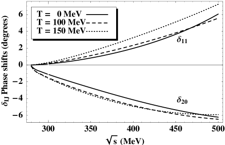
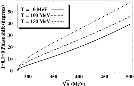
Figure 1: Temperature evolution of the phase shifts $\delta_{IJ}$ for $IJ=11,00,20$.

The $IJ=11$ channel is particularly interesting, since it is dominated by the $\rho$ resonance, whose thermal deformation has been related to the anomalous dilepton spectra in RHIC [10, 11]. By analyzing this channel at low energies, we are studying the tail of the resonance. The low-energy temperature enhancement of the phase shift can then be interpreted as a stronger thermal effect of the rho, although with pure ChPT calculations we cannot disentangle whether it is due to a larger width or to a smaller mass. Qualitatively, the chiral combination of parameters that dominate the phase shift in this channel is $\bar{l}_{1}-\bar{l}_{2}\sim\Gamma_{\rho}f^{4}/M_{\rho}^{5}$, following the resonance saturation hypothesis [2, 19]. In order to obtain larger phase shifts at $T=0$, we need somewhat larger $\bar{l}_{1}-\bar{l}_{2}$ values. Thus, the low-energy thermal phase shifts would correspond at $T=0$ to a larger $\Gamma_{\rho}f^{4}/M_{\rho}^{5}$ ratio, although with the $T=0$ part only we cannot mimic accurately the low-energy thermal behavior. Therefore, our results are consistent with most models that expect a low-$T$ sizable thermal increase of the rho width due to the thermal increase of phase space, with an almost constant thermal $M_{\rho}$ [20, 11]. Our model independent perturbative result is confirmed by our discussion at the end of section 2.3 and by the unitarized results in [12].

In conclusion, we have calculated the $\pi\pi$ scattering to one loop in Chiral Perturbation Theory at finite temperature $T$. Our thermal amplitude has been calculated with $T=0$ asymptotic states and the thermal ITF Green function, whose analytic continuation corresponds to the retarded RTF Green function, which has a suitable causal and analytic structure. Despite the loss of Lorentz covariance of the thermal formalism, any $\pi\pi$ elastic amplitude can still be related to a single one by means of a generalized crossing symmetry in terms of the external four-momenta. We have found the thermal generalization of perturbative partial wave unitarity to one loop, which amounts to replacing the $T=0$ two-particle phase space with its thermal version. This accounts for emission and absorption of pion pairs inside the thermal bath, providing a physical interpretation of the imaginary part of the thermal amplitude and giving the expected analytic structure above threshold, consistently with causality and thermal unitarity. We have checked that our amplitudes satisfy this constraint. With these amplitudes, we have studied the low energy behavior of thermal $\pi\pi$ elastic scattering in a model independent formalism, finding an enhanced phase shift in all channels, as dictated by the thermal phase space, but with little change in the modulus of the partial waves. Physically, this means that one cannot mimic the low-$T$ behaviour of dynamical quantities just by scaling $f_{\pi}\rightarrow f_{\pi}(T)$.

One of the main physical observables that can be related to our thermal scattering amplitude are the masses and widths of the $\rho$ and $\sigma$ mesons [12]. We have given here a low-$T$ qualitative description for the case of the $\rho$. Further quantitative and detailed information can be obtained if these results are extended to higher energies beyond pure ChPT. In particular, by means of unitarization methods [13] that generate dynamically light resonances like the $\rho$ and $\sigma$ mesons [12]. Hence, our results are useful as a starting point for the description of relevant physical processes where chiral symmetry and unitarity play a crucial role, such as the properties of those resonances in the plasma formed after a Relativistic Heavy Ion Collision.

Acknowledgments

The authors thank A. Dobado for useful comments and discussions. F. J. Ll-E thanks P. Bicudo, S. Cotanch, P. Maris, E. Ribeiro and A. Szczepaniak too. Work supported from the Spanish CICYT projects, FPA2000-0956,PB98-0782 and BFM2000-1326.

Appendix A Loop integrals

The following are the integrals needed for our calculation in an arbitrary reference frame (not necessarily the c.o.m frame, where pions are at rest with the thermal bath). The signature of the metric in Euclidean space is $(-\ -\ -\ -)$ and we will use the notation

$$\int_{\beta}\frac{d^{D}q}{(2\pi)^{D}}\equiv\frac{1}{\beta}\sum_{n=-\infty}^{n=+\infty}\int\frac{d^{D-1}q}{(2\pi)^{D-1}}$$

where $\beta=1/T$, $q_{0}=2\pi nT$ and $Q_{0}=2\pi kT$ with $k$ integer denotes an external frequency. Also we denote $\Delta G(T)\equiv G(T)-G(T=0)$. First, we have the tadpole integral:

$$F_{\beta}\equiv\int_{\beta}\frac{d^{D}q}{(2\pi)^{D}}\frac{1}{q^{2}-m^{2}}\ .$$ (13)

Then, three integrals of pion loops with an external momentum flow:

$$J_{k}(Q_{0},|\vec{Q}|;T) \equiv \int_{\beta}\frac{d^{D}q}{(2\pi)^{D}}\frac{q_{0}^{k}}{(q^{2}-m^{2})((q-Q)^{2}-m^{2})}\ ,\quad k=0,1,2$$ (14)

All other integrals with momenta in the numerator can be reduced to those four as

$$\int_{\beta}\frac{d^{D}q}{(2\pi)^{D}}\frac{q_{i}}{(q^{2}-m^{2})((q-Q)^{2}-m^{2})} = -\frac{Q_{i}}{\arrowvert\vec{Q}\arrowvert^{2}}\left[Q_{0}J_{1}+\frac{1}{2}J_{0}Q^{2}\right]\ .$$ (15)

$$\int_{\beta}\frac{d^{D}q}{(2\pi)^{D}}\frac{q_{\mu}Q^{\mu}}{(q^{2}-m^{2})((q-Q)^{2}-m^{2})} = \frac{Q^{2}}{2}J_{0}\ .\$$ (16)

$$\int_{\beta}\frac{d^{D}q}{(2\pi)^{D}}\frac{q_{0}q_{i}}{(q^{2}-m^{2})((q-Q)^{2}-m^{2})} = -\frac{Q_{i}}{\arrowvert\vec{Q}\arrowvert^{2}}\left[Q_{0}J_{2}+\frac{Q^{2}}{2}J_{1}+\frac{Q_{0}}{2}F_{\beta}\right]\ .$$ (17)

$$\int_{\beta}\frac{d^{D}q}{(2\pi)^{D}}\frac{q_{i}q_{j}}{(q^{2}-m^{2})((q-Q)^{2}-m^{2})} = Q_{i}Q_{j}I_{2a}+g_{ij}I_{2b}$$ (18)

$$\int_{\beta}\frac{d^{D}q}{(2\pi)^{D}}\frac{q_{0}q\!\cdot\!q}{(q^{2}-m^{2})((q-Q)^{2}-m^{2})} = Q_{0}F_{\beta}+m^{2}J_{1}$$ (19)

$$\int_{\beta}\frac{d^{D}q}{(2\pi)^{D}}\frac{q_{i}q\!\cdot\!q}{(q^{2}-m^{2})((q-Q)^{2}-m^{2})} = Q_{i}F_{\beta}-m^{2}\frac{Q_{i}}{\arrowvert\vec{Q}\arrowvert^{2}}\left(Q_{0}J_{1}+\frac{Q^{2}}{2}J_{0}\right)\ .$$ (20)

$$\int_{\beta}\frac{d^{D}q}{(2\pi)^{D}}\frac{(q\!\cdot\!q)^{2}}{(q^{2}-m^{2})((q-Q)^{2}-m^{2})}=(Q^{2}+2m^{2})F_{\beta}+m^{4}J_{0}\ .$$ (21)

where

$$I_{2a}(Q) = \frac{1}{(D-2)\arrowvert\vec{Q}\arrowvert^{4}}\left[\left((D-1)Q_{0}^{2}+\arrowvert\vec{Q}\arrowvert^{2}\right)J_{2}+(D-1)Q_{0}Q^{2}J_{1}+\left(\frac{D-1}{4}Q^{4}+m^{2}\arrowvert\vec{Q}\arrowvert^{2}\right)J_{0}\right.$$

$$+ \left.\left((\frac{Q^{2}}{2}+Q_{0}^{2})(D-1)+\arrowvert\vec{Q}\arrowvert^{2}\right)F_{\beta}\right]$$

$$I_{2b}(Q) = \frac{1}{(D-2)\arrowvert\vec{Q}\arrowvert^{2}}\left[-Q^{2}J_{2}+Q_{0}Q^{2}J_{1}+\left(\frac{Q^{4}}{4}+m^{2}\arrowvert\vec{Q}\arrowvert^{2}\right)J_{0}-\frac{Q^{2}}{2}F_{\beta}\right]\ .$$ (22)

The above integrals have the appropriate $T\longrightarrow 0$, $m\longrightarrow 0$ limits and at $T=0$ they can be written just in terms of the tadpole $F$ and $J_{0}$ [2]. Recall that all the UV divergences of the $F_{\beta}$ and $J$ integrals are contained in the $T=0$ part, since $\Delta F$ and $\Delta J_{k}$ always contain Bose-Einstein functions vanishing exponentially for large momentum. Therefore, using dimensional regularization, we always separate the $T=0$ part, regularized and renormalized as in [2] and set $D=4$ in $\Delta F_{\beta}$ and $\Delta J_{k}$.

The functions $J_{k}$ in eq.(14) can be analytically continued after performing the Matsubara sums. All the Euclidean discrete frequencies are then continued to $-iE$ with $E$ real and continuous, i.e,

$$J_{k}(Q_{0},|\vec{Q}|;T) \rightarrow (-i)^{k}\,J_{k}(-iE,|\vec{Q}|;T)$$ (23)

In the c.o.m. frame the imaginary part of the $J$ integrals, can be calculated exactly, e.g, eq.(10). When the c.o.m frame $|\vec{{\bf S}}|={\bf T_{0}}={\bf U_{0}}=0$, coincides with the thermal bath rest frame, only $F_{\beta}$, $J_{0}({\bf S})$, $J_{0}({\bf T})$, $J_{2}({\bf T})$ have to be evaluated (note that $J_{0}({\bf U})$, $J_{2}({\bf U})$ can be computed from the corresponding ${\bf T}$ integrals). Specifically

$$J_{2}({\bf S}) = \frac{{\bf S_{0}}^{2}}{4}J_{0}({\bf S})+\frac{F_{\beta}}{2}\ ,\quad J_{1}({\bf S})=\frac{{\bf S_{0}}}{2}J_{0}({\bf S})\ ,\quad J_{1}({\bf T})=0$$ (24)

The real part of $\Delta J_{0}$ analytically continued as in eq.(23) in the $S$-channel reads

$$\mbox{Re}\,\Delta J_{0}({\bf S})=-\frac{1}{\pi^{2}}PV\int_{m}^{\infty}dE\ \frac{q(E)n(E)}{s-4E^{2}}$$ (25)

where $q(E)=\sqrt{E^{2}-m^{2}}$ $n(E)=\left(e^{\beta E}-1\right)^{-1}$ and $PV$ denotes Cauchy’s Principal Value. Note that the above expression is valid for $\omega$ real ($s=\omega^{2}$) and the pole of the integrand is only present for $s>4m^{2}$, where $\mbox{Im}\,J_{0}\neq 0$. Finally, in the $T(U)$ channels, we get

$$\Delta J_{k}(\arrowvert\vec{{\bf T}}\arrowvert) = \frac{1}{8\pi^{2}}\int_{0}^{\infty}dq\frac{q\,n(E_{q})\,E_{q}^{k-1}}{\arrowvert\vec{{\bf T}}\arrowvert}\log\left(\frac{2q+\arrowvert\vec{{\bf T}}\arrowvert}{2q-\arrowvert\vec{{\bf T}}\arrowvert}\right)^{2},\qquad k=0,2$$

where $E_{q}^{2}=q^{2}+m^{2}$. The above result is valid for real $\arrowvert\vec{{\bf T}}\arrowvert$ (or $s>4m_{\pi}^{2}$ for $\pi\pi$ scattering).

References

- [1] S. Weinberg, PhysicaA 96, 327 (1979).
- [2] J. Gasser and H. Leutwyler, Annals Phys. 158, 142 (1984); Nucl. Phys. B 250, 465 (1985).
- [3] J. Gasser and H. Leutwyler, Phys. Lett. B 184, 83 (1987); P. Gerber and H. Leutwyler, Nucl. Phys. B 321, 387 (1989); A. Schenk, Phys. Rev. D 47, 5138 (1993).
- [4] S.Chiku and T.Hatsuda, Phys. Rev. D 57, R6 (1998).
- [5] D.Jido, T.Hatsuda and T.Kunihiro, Phys. Rev. D 63, 011901(R) (2000).
- [6] Y. B. He, J. Hufner, S. P. Klevansky and P. Rehberg, Nucl. Phys. A 630, 719 (1998).
- [7] N. Kaiser, Phys. Rev. C 59 (1999) 2945.
- [8] E. Quack, P. Zhuang, Y. Kalinovsky, S. P. Klevansky and J. Hufner, Phys. Lett. B 348, 1 (1995).
- [9] B. Lenkeit et al. [CERES-Collaboration], Nucl. Phys. A 661, 23 (1999)
- [10] G. Q. Li, C. M. Ko and G. E. Brown, Phys. Rev. Lett. 75, 4007 (1995)
- [11] V. L. Eletsky, M. Belkacem, P. J. Ellis and J. I. Kapusta, Phys. Rev. C 64, 035202 (2001)
- [12] A.Dobado, A.Gómez Nicola, F.J.Llanes-Estrada and J.R.Peláez, arXiv:hep-ph/0206238.
- [13] T. N. Truong, Phys. Rev. Lett. 67, 2260 (1991); A. Dobado, M. J. Herrero and T. N. Truong, Phys. Lett. B 235, 134 (1990); A. Dobado and J. R. Pelaez, Phys. Rev. D 56, 3057 (1997).
- [14] M.Le Bellac, Thermal Field Theory (Cambridge University Press, 1996) and references therein.
- [15] R.Baier and A.Niégawa, Phys.Rev. D 49 (1994) 4107.
- [16] R.Kobes, Phys.Rev.D 42 (1990) 562; 43 (1991) 1269.
- [17] A.Niégawa Phys.Lett. B 247 (1990) 351; Phys.Rev. D 57 (1998) 1379. N.Ashida, H.Nakkagawa, A.Niégawa and H.Yokota, Phys.Rev. D 45 (1992) 2066; Ann.Phys. (N.Y.) 215 (1992) 315; 230 (1994) 161 (E).
- [18] H. A. Weldon, Phys. Rev. D 28, 2007 (1983); Annals Phys. 214, 152 (1992).
- [19] J.F.Donoghue, C.Ramirez and G.Valencia, Phys. Rev. D39, 1947 (1989); G. Ecker, J. Gasser, A. Pich and E. de Rafael, Nucl. Phys. B 321 311 (1989).
- [20] C. A. Dominguez, M. Loewe and J. C. Rojas, Z. Phys. C 59, 63 (1993); R. D. Pisarski, Phys. Rev. D 52, 3773 (1995).