Goldstone excitations from spinodal instability

Abstract

The squared mass of a complex scalar field is turned dynamically into negative by its $O(2)$-invariant coupling to a real field slowly rolling down in a quadratic potential. The emergence of gapless excitations is studied in real time simulations after spinodal instability occurs. Careful tests demonstrate that the Goldstone modes appear almost instantly after the symmetry breaking is over, much before thermal equilibrium is established.

1 Introduction

This investigation is the first stage of a complex study with the aim to explore in detail the mechanism of the energy transfer to the Higgs field at the end of the inflationary period of the Universe as it is anticipated in scenarios of hybrid inflation [1, 2].

The $O(2)$-symmetric model used in studies of hybrid inflation has the following Lagrangian density for the real scalar (“inflaton”) field $\psi$ and the complex (“Higgs”) field $\Phi=\Phi_{1}+i\Phi_{2}$:

$$L={1\over 2}(\partial_{\nu}\psi(x))^{2}-{1\over 2}m_{\psi}^{2}\psi^{2}+{1\over 2}|\partial_{\nu}\Phi(x)|^{2}-{1\over 2}m_{\Phi}^{2}|\Phi|^{2}-{\lambda\over 24}|\Phi|^{4}-{1\over 2}g^{2}\psi^{2}|\Phi|^{2},$$ (1)

where $m_{\Phi}^{2}$ has the wrong sign.

At the beginning the energy density is carried partly by the inflaton field due to its $\sim{\cal O}(M_{P})$ initial amplitude and partly by the potential energy of the Higgs-field which starts at the symmetric maximum. It is transformed very efficiently into kinetic and gradient energy densities when the squared effective mass of the Higgs field becomes negative and the modes of the complex field with low spatial frequency $|{\bf k}|<|M_{eff}|$ start to increase exponentially due to the spinodal instability [3]. The Higgs field eventually arrives to a symmetry breaking ground state, on its top with massive and massless thermal excitations.

The present study was carried out in Minkowski metrics and with classical fields starting from an initial state corresponding to the above situation. Therefore at this stage the results have more relevance to non-equilibrium phase transitions in relativistic field theoretical models than to cosmology. The results will serve as reference for future simulations to be performed in an expanding FRW-geometry. Our study was inspired by recent papers of Felder et al. describing also the evolution of a complex Higgs field after a sudden change of sign of its squared mass [3, 4].

Very recently a detailed study concentrating on the statistics of defect formation was published [5], where the change of sign in the mass of the Higgs field is induced by the free motion of a homogenous real scalar field. The present work represents a complementary approach since we study rather the elementary excitations of the system than extended objects.

Our aim is to investigate systematically the way the different components of the complex Higgs field are excited. Special attention is paid to the real time appearance of the Goldstone mode after the period of spinodal instabilities. Analogous question was analyzed recently by Boyanovsky et al. [6] and by Baacke and Heitmann [7] in the infinite component (large $N$) limit of the quantum dynamics. They solved the coupled set of the renormalised equations of motion of the order parameter and of the to-be-Goldstone modes following a squared mass quench. The effective mass square governing the mode equations of the Goldstone fluctuations was analyzed which depends non-linearly on the actual value of the order parameter and reflects also the global back-reaction of the Goldstone-modes. It was found that the squared mass of the ”pion” modes starts to oscillate around the asymptotic zero value rather early, but the oscillations are damped only for asymptotically large times as $t^{-1}$. In a recent paper [8] renormalised non-equilibrium gap equations were solved for the effective mass-squares of the longitudinal and transversal modes propagating on a time dependent background. These masses were in earlier papers [9, 10] with a self-consistent parametrisation of the corresponding propagators. It turned out that the time-dependent variational mass-squares do not obey the Goldstone theorem away from equilibrium. It will be interesting to compare these semi-analytical approximate investigations with the direct mass measurements performed in numerical simulations of $O(N)$ symmetric systems.

The classical (cut-off) field theory provides a useful point of reference, since gapless excitations are present in its broken symmetry phase near equilibrium. Our numerical results for $N=2$ hint at an essentially different picture on the real time genesis of the Goldstone modes.

The presentation of our results is organised in the following way. Section 2 summarizes the set of parameters used in and the algorithmical details applied to the numerical solution. Our detailed discussion is divided into two parts. In section 3 the methods for finding the independently moving degrees of freedom are presented. There we give direct evidence for the early presence of massless excitations. In section 4 the process of thermalisation is described, pointing out the slow damping of angular O(2) oscillations, supporting the presence of Goldstone modes. Section 5 contains our conclusions.

2 Lagrangian parameters, initial conditions and discretisation

The parameters we choose for the present investigation imitate a situation which would be characteristic for a GUT-like transition. In lattice units the Higgs particle has unit squared mass parameter (with the wrong sign), the inflaton mass square is $10^{-3}$ times smaller. The initial amplitude of the inflaton is large: $\psi_{0}=15$. Variation of its value does not influence the qualitative features of the time evolution of the system until its contribution to the potential energy is negligible relative to the initial energy content of the Higgs field.

A very weak nonlinearity $\lambda=24\times 10^{-4}$ was fixed in order to facilitate the comparison of our results with [4]. In this way the dominant part of the initial energy was stored in the Higgs potential. When we varied $\psi_{0}$ in a range, without changing the dominant component of the potential energy, no change was experienced in the thermalisation scenario after the spinodal instability. The use of a stronger Higgs self-coupling does not seem to have any qualitative consequence on the features of the appearance of Goldstone modes.

The initial space average of the Higgs field was fixed to zero. To the two real components of the complex field at every site a (white noise) amplitude evenly distributed on the $[-1,1]\times 10^{-4}$ interval was assigned. The amplitude of this random noise can be used to control which phase the system finally relaxes to. With the present choice the final value of $|\Phi|$ is very close to the classical minimum of the Higgs potential, the system is very cold. One needs 5 order of magnitude stronger noise to drive the system into the symmetric phase.

Runs starting with different initial noise seeds were used to assess the statistical errors of the mass-values extracted. The restricted number of runs (6-14 depending on the size of the system), might cause some underestimation of the errors.

The value of the inflaton-Higgs coupling used in the present investigation is $g^{2}=10^{-2}$. It turned out in our numerical studies that with stronger coupling (for $g^{2}\geq 8\times 10^{-2}$) the time necessary for the full development of the spinodal instability takes several oscillation periods of the inflaton, and the growth of unstable modes can happen only during the passage of the inflaton field through zero. This behaviour can be understood with help of the theory of broad parametric resonance developed in [11] when it is applied to a system where also spinodal instability can occur. The main reason for this phenomenon is the fact that with the increase of $g^{2}$ the time interval of the non-adiabatic inflaton evolution becomes shorter. Its discussion is beyond the scope of the present paper. It has been checked that the spectral characterisation of the different modes as they appear after the spinodal instability are independent of $g^{2}$.

We have followed the temporal evolution of the inflaton as well as of the $O(2)$-field on a spatial lattice with the equations written for dimensionless field quantities:

$$\ddot{\psi}(x)-\bigtriangleup\psi(x)+{m_{\psi}^{2}\over m_{d}^{2}}\psi(x)+g^{2}\Phi^{2}\psi=0$$

$$\ddot{\Phi}_{i}(x)-\bigtriangleup\Phi_{i}(x)+{m^{2}_{\Phi}\over m_{d}^{2}}\Phi_{i}(x)+{\lambda\over 6}|\Phi(x)|^{2}\Phi_{i}(x)+g^{2}\psi^{2}\Phi_{i}=0$$ (2)

with the scaled quantities

$${m^{2}_{\Phi}\over m_{d}^{2}}=-1,\qquad{m^{2}_{\psi}\over m^{2}_{d}}=0.001,$$

$${\psi_{d}\over m_{d}}=\psi,\quad{\Phi_{d}\over m_{d}}=\Phi,\quad t_{d}m_{d}=t,\quad a_{d}m_{d}=a\equiv 1$$ (3)

(the symbols with index $d$ refer to dimensionfull quantities).

The characteristic time scales related to the elementary excitations turned out much shorter than the relaxation times, especially for the long wavelength Goldstone modes. This circumstance made the choice of the time-step in the standard leapfrog algorithm used by us a sensitive issue. The stability of the algorithm was ensured by choosing the time step in the interval $0.125\geq a_{t}/a_{s}\geq 0.0625$. The long term stability of the time evolution was controlled by monitoring the conservation of the energy and the $O(2)$ charge of the system. Due to the initial conditions the latter was fixed at zero. The charge density for the above time step was fluctuating around zero with an amplitude $\sim 0.04$, but in selected runs using hundred times shorter time steps we could reach an amplitude ${\cal O}(10^{-4})$ with unchanged qualitative features.

3 Finding the independent excitations

The spinodal instability driving the Higgs field from the symmetric phase to the broken symmetry state was investigated on lattices with increasing $L^{3}=32^{3},64^{3},128^{3}$ volumes and with periodic spatial boundary conditions. Due to our initial “white noise” amplitude distribution the system chooses a well-defined (though random) direction in the $O(2)$ internal space contrary to the case studied by [4] where the space average of the Higgs field stayed at the origin.

The coincidence of the change of sign of the instant effective squared mass $M^{2}_{eff}$ with the start of the spinodal instability is investigated in Fig.1. Various alternative definitions of the effective Higgs mass are used:

$$M_{eff,1}^{2} = m_{\Phi}^{2}+g^{2}\langle\psi\rangle^{2}(t),$$

$$M_{eff,2}^{2} = M_{eff,1}^{2}+g^{2}\langle(\psi-\langle\psi\rangle)^{2}\rangle,$$

$$M_{eff,3}^{2} = M_{eff,2}^{2}+{\lambda\over 2}\langle|\Phi|^{2}\rangle.$$ (4)

The brackets mean spatial averaging.

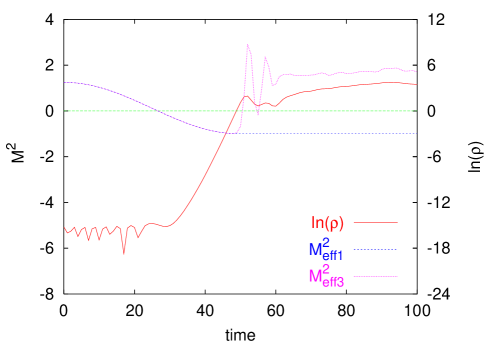
Figure 1: Time evolution of $\rho(t)$ (the space average of $|\Phi({\bf x},t)|^{2}$) and of the various definitions of $M^{2}_{eff}$ (see Eq.(4))

The first definition, where one assumes that the fluctuations of the $\psi$-field are negligible is used in most discussions of hybrid inflation. It predicts a change of sign when the inflaton reaches the critical value $\psi_{c}=|m_{\Phi}|/g$, and was ensured to be valid in [5] by setting $m_{\psi}^{2}=0$. In the present case the inflaton rolls in a harmonic potential and one can test if the fluctuations of the $\psi$ and $\Phi$ fields have any effect at the start of the spinodal instability. In the Figure only $M^{2}_{eff,1}$ and $M^{2}_{eff,3}$ are displayed, since $M^{2}_{eff,2}$ is indistinguishable from the first one. The deviation of the two versions of the mass appears near the end of the instability, when $M^{2}_{eff,1}$ stabilizes at the value $-1$, while $M^{2}_{eff,3}$ approaches a positive stationary value after wild oscillations. The increase of the order parameter $\rho\equiv\int d^{3}x|\Phi|/V$ becomes noticeable with a slight time delay after the sign-change of the effective Higgs mass. This is due to the gradual increase of $-M^{2}_{eff,1}$. The spinodal increase of the order parameter is exponential, with a slowly varying slope. Near the saturation of the order parameter the slope is very close to the unit value expected with our choice of $-m_{\Phi}^{2}$.

Next, we turn to the separation of the independently oscillating degrees of freedom. At every lattice point the complex field can be represented as $\Phi({\bf x},t)=\rho({\bf x},t)\exp(i\varphi({\bf x},t))$. The main question of this investigation was, at what time the radial and angular Higgs variables become dinamically independent. This can be monitored by calculating the temporal variation of the elements of the “velocity”-correlation matrix $W_{ij}(t)$, which was constructed the following way.

Let us define the 3-component quantity: $v_{i}({\bf x},t)=\{\dot{\rho}({\bf x},t),\rho({\bf x},t)\dot{\varphi}({\bf x},t),\dot{\psi}({\bf x},t)\}$ and form the spatial fluctuation matrix

$$W_{ij}={\tilde{W}_{ij}\over\tilde{W}^{1/2}_{ii}\tilde{W}^{1/2}_{jj}},\qquad\tilde{W}_{ij}(t)={1\over V}\int d^{3}xv_{i}({\bf x},t)v_{j}({\bf x},t)-{1\over V}\int d^{3}xv_{i}({\bf x},t){1\over V}\int d^{3}xv_{j}({\bf x},t).$$ (5)

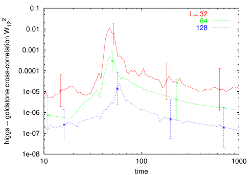
Figure 2: Time evolution of the square of the normalised cross-correlation coefficient $W_{12}(t)$ on a sequence of different size lattices

In Fig.2 we show the early time variation of the $W_{12}(t)$ element on three different size lattices. One observes that the level of Higgs-Goldstone cross-correlation decreases by about two orders of magnitude from lattice size $L=32$ to $L=128$. All non-diagonal correlation coefficients show maxima during the spinodal instability. In case of $W_{13}(t)$ it was found that the maximum of the inflaton-Higgs cross-correlation coefficient is independent of the size and is ${\cal O}(1)$. In case of $W_{12}$ and $W_{13}$ also the maximum decreases with the size of the system. It is unclear what is the thermodynamical limit of this maximum reached during the spinodal instability.

After the saturation of the unstable modes the average level of all off-diagonal elements of the normalized correlation matrix stabilizes for $L=128$ at ${\cal O}(10^{-7})$. This level of decoupling is reached the slowest for $W_{12}$. Therefore the radial and angular motion of the $O(2)$-field in the internal space can be considered with very good accuracy as independent starting from about $t\sim 200$. The analysis gives very similar results when applied directly to the polar coordinates: $x_{i}=\{\rho,\varphi,\psi\}$.

This analysis provides the basis for a separate application of various methods of mass determination to each of the three independent coordinates. Would the cross-correlations be ${\cal O}(1)$ beyond the instability, one could not avoid the application of a complicated diagonalisation process before applying the methods of dispersive mass determination to be described next.

The method developed and tested by us on the example of the one-component scalar field [12] has been further improved for the non-trivial task of the investigation of Goldstone modes. Its present algorithm is summarised in the following.

One keeps track of the time evolution of the lower-$k$ spatial Fourier transform of all three $v$-type lattice fields. No binning is applied. Next, one computes the frequency-spectra of the time evolution of the power of the single $k$-modes. They show several peaks and the strongest one was identified with the eigenfrequency of the investigated ${\bf k}$-mode (the others correspond to various forced oscillation modes). This correspondence yields the dispersion relation $\omega({\bf k})$.

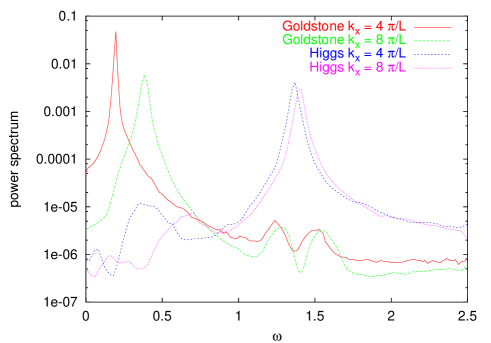
Figure 3: Temporal Fourier spectra of the $k_{x}=4\pi/L,8\pi/L,k_{y}=k_{z}=0$ modes derived from long (near equilibrium) time evolution

In equilibrium systems we verified the correctness of this method by taking long time intervals. In Fig.3 such spectra are displayed for the lowest two ${\bf k}$ modes for both the Higgs and the Goldstone variable on the largest $L=128$ lattice. We observed essentially no volume dependence. The straight line extrapolation of the dispersion relation from finite ${\bf k}$ modes towards zero wave number is of very good quality and shows the absence of any gap in case of the angular mode. The Higgs-mode follows a massive relativistic dispersion relation.

It was checked that the analysis of shorter time intervals down to $T=32|m_{\Phi}|^{-1}$ results in masses which are in good agreement with spectra obtained with much finer $\omega$ resolution.

Far from equilibrium fields vary fairly fast, any analysis averaged over a long time interval misses the changes which occur on short time scales. With the present choice of the parameters a fast Fourier analysis (FFT) using $T/|m_{\Phi}|=32$ allows an accurate enough determination of the Fourier coefficients in the interval $\omega\in(2\pi/T,12\pi/T)$. 14 independent runs were analysed on an $L=128$ lattice. The masses were obtained by subtracting the lattice $|{\bf k}|^{2}$ from the corresponding $\omega^{2}$ for 9 modes, and fitting the remaining numbers to a constant. The average standard deviation of the fits performed in different moments is shown as an error estimate of the mass determination. Fig.4 displays the time evolution of the independent inflaton, Higgs and Goldstone masses.

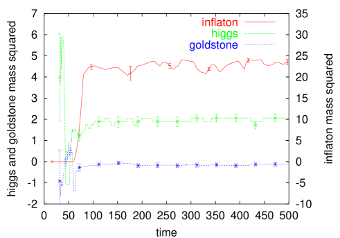
Figure 4: The variation of the masses of the Higgs-, Goldstone- and inflaton excitations derived from the direct dispersion relation method

In an earlier version of this method [12] we have assumed that all ${\bf k}$-modes oscillate with a single eigenfrequency. Then from the ratio $|\dot{x}_{i}({\bf k})|^{2}/|x_{i}({\bf k})|^{2}$ formed with help of $x$-type variables one can deduce the dominant frequency. In order to minimize fluctuations the numerator and the denominator were averaged separately over the modes lying in narrow $|{{\bf k}}|$ bins. The squared frequency was linearly extrapolated to $|{\bf k}|=0$ and the limiting value identified with the squared mass.

In Fig.5 one can see that the masses determined with this method provide for both components slightly higher values than the improved method. Their temporal fluctuations quickly diminish with increasing lattice size. The mass estimates shown in these figures represent averages of 40 independent runs for $L=32$ (9 runs were analysed for $L=64$, and 6 for $L=128$ with no sizable finite size dependence). The error bars displayed at the right hand side of both figures represents the standard deviation of the squared masses. Within these limitations on the accuracy the results of the two mass determinations are compatible.

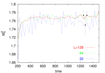
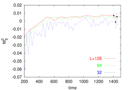
Figure 5: Time evolution of the masses of the Higgs (Goldstone) excitations derived from the ratio of the kinetic to the amplitude power spectra of the corresponding field combinations

For the Goldstone mode the best fit was reached by analyzing the phase factor $|\dot{X}_{k}|^{2}/|X_{k}|^{2},~{}X=\exp(i\varphi)$. This choice was suggested by the idea of non-linear $\sigma$-models. We note that only modes with $|{\bf k}|\geq 0.5$ were included into the analysis. As we will discuss in the next section for lower wave numbers the Goldstone modes are highly excited during and after the instability. They relax very slowly, and their motion does not seem to follow a single eigenfrequency. From the right hand picture of Fig.5 one recognizes an apparent (rather small) negative squared mass fit for a short time interval directly after the spinodal instability. For later times the fit is compatible with vanishing mass.

We conclude this section with the statement that Goldstone modes are present in the excitation spectra of the model very early. The important question to be discussed in the next section is the degree of excitation of this mode relative to the others, that is the part of energy carried by the light modes.

4 Thermalisation and Goldstone-damping

The temporal evolution of the kinetic power spectra reflects very well the approach to classical thermal equilibrium, characterized by the equipartition of the energy. In Fig.6 the flattening of the kinetic Goldstone power spectra in the region $k\geq 1$ is clearly observed. The low ${\bf k}$ peak has an almost time independent height in the interval $t=(100,1500)$, its decrease is well recognizable only for $t\sim 10^{5}$.

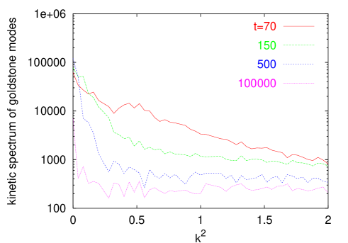
Figure 6: The evolution of the Goldstone kinetic power spectrum in time reveals the fast approach of high-$k$ modes towards equipartition and the slow relaxation in the low-$k$ part of the spectrum

This observation is probably the most appealing result of the present investigation. Below we attempt its semiquantitative interpretation with help of a combination of perturbative and non-perturbative arguments.

In a recent publication ([13], Appendix B and C) we have presented the perturbative evaluation of the Goldstone and Higgs damping rates in the broken phase of a classical(!) $O(N)$ symmetric field theory. The analysis was performed for constant value of the order parameter. The Goldstone and Higgs modes were characterized by constant mass values and by uncorrelated spectral functions

$$\Delta_{a}(p)=2\pi\epsilon(p_{0})\delta(p^{2}-M^{2}_{a})f_{a}(p_{0}),\qquad a=H,G.$$ (6)

The induced source densities for these equations were found iteratively, assuming weak non-linearities in the system. The “self-energy” terms of the two types of excitations were established by taking into account the solution with just one iteration. The following explicit expressions were found:

$$\Pi_{H}(p) = (\lambda\Phi)^{2}\Bigl{[}R_{HH}(p)+{N-1\over 9}R_{GG}(p)\Bigr{]},\qquad\Pi_{G}(p)=\bigl{(}{\lambda\Phi\over 3}\bigr{)}^{2}2R_{GH}(p),$$

$$R_{ab} = \int{d^{4}q\over(2\pi)^{4}}\bigl{(}\Delta_{b}(q-p/2)-\Delta_{a}(q+p/2)\bigr{)}{1\over 2qp-M_{b}^{2}+M_{a}^{2}}.$$ (7)

In equilibrium systems the classical “number”-distribution is given by $f_{a}(q_{0})=T/q_{0}$. The damping rates are determined by the imaginary parts of the self-energies.

The initial conditions generated by the spinodal instability for the later evolution is hard to specify explicitly. In principle one can attempt the numerical determination of the spectral function of each of the independent degrees of freedom [14, 15]. Here we followed a less systematic path based on the phenomenological description of the actual system presented in the preceding section, which confirms the presence of separate Higgs and Goldstone degrees of freedom with well-defined masses in our $O(2)$ invariant system shortly after the spinodal instability is over. Therefore we accept for the spectral densities the form of a free gas for each of them. Then the only remaining task is to find the nonequilibrium generalisation of the distribution functions $f_{a}$.

A classical analogue of the average occupation number was extensively used for the dynamical coordinate $X_{a}$ in [4]:

$${\cal F}_{a}(\omega_{k})={1\over\omega_{k}}(|\dot{X}_{a}({\bf k})|^{2}+\omega_{a}({\bf k})^{2}|X_{a}(k)|^{2}),\qquad\omega_{a}(k)^{2}={\bf k}^{2}+M_{a}^{2}.$$ (8)

It was computed here (see Fig.7) for the absolute value and the phase factor of the complex field. We see that the “number density” of the Higgs degree of freedom which initially decreases exponentially at later times approaches uniformly the $1/\omega_{k}$ regime. Also the virial equilibrium of the corresponding kinetic and potential contributions is fulfilled very early (for $t\sim 500$). In case of the Goldstone degree of freedom the convergence to the classical “number” density is not uniform, the excitation of the low-$k$ modes remains strong, and the approach to the classical regime in the high-$k$ region is slower.

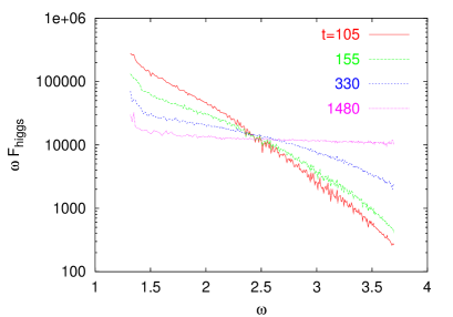
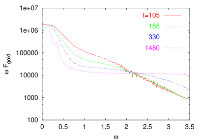
Figure 7: The evolution of $\omega\times{\cal F}_{a}(\omega)$ of the Higgs (left) and Goldstone (right) modes shortly after the spinodal instability is saturated

The smoothness of ${\cal F}_{a}$ and the thermalisation tendency observed in their evolution leads us to the conjecture that the form (6) of $\Delta_{a}(p)$ remains valid in the present case, only the functions $f_{a}$ are replaced by a far-from-equilibrium form. With this assumption we can use the method of evaluation described in Appendix C of [13]. (One should be aware of the fact that beyond the present one-loop estimation the use of the proposed non-equilibrium form of $\Delta_{a}(p)$ would lead to pinch singularities [16]). In case of the Goldstone modes we find the following expression for the on-shell damping rate:

$$\Gamma_{G}(k_{0}=|{\bf k}|)=\bigl{(}{\lambda\Phi\over 3}\bigr{)}^{2}{1\over 32\pi|{\bf k}|^{2}}\int_{M_{H}^{2}/4|{\bf k}|}^{\infty}dp_{0}[{\cal F}_{G}(p_{0})-{\cal F}_{H}(p_{0}+k_{0})].$$ (9)

The lower limit is a direct kinematical consequence of the zero mass nature of the Goldstone mode. It restricts the contribution to the large frequency tails of both distributions if the damping rate of the low-$k$ modes is to be estimated. Since these modes are filled very late after the spinodal instability is complete, the damping of these Goldstone modes is very inefficient.

It is amusing that the far-equilibrium classical evolution under specific initial conditions produces a phenomenon for the Goldstone excitation, which occurs at equilibrium in the quantum version of the model due to the exponentially small high frequency tail of the Bose-Einstein factor [17, 13, 18].

Due to the rather strong initial excitation of the low-$k$ Goldstone modes, the average kinetic energy stored in this degree of freedom is the biggest directly after spinodal instability. This averaging, however, is somewhat misleading. By subtracting the energy of the modes participating in the low-$k$ peak, the temperature of the ”equlibrated” modes appears somewhat lower than the corresponding Higgs-temperature. With time a metastable ”equilibration” between these modes becomes almost complete, as one can see in Fig.8.

This means that the equilibration in the $O(2)$ configuration space is much more efficient, than the energy transfer to the inflaton. Apparently, the inflaton field is frozen at a much lower temperature than the $O(2)$ fields.

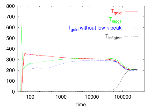
Figure 8: The thermal history of the independent degrees of freedom as calculated from their average kinetic energies

The time spent by the inflaton in frozen state is of the same order of the magnitude as the relaxation time of the Goldstone low-$k$ peak. We have checked that with the increase of $g^{2}$ the inflaton temperature starts to increase earlier, but the transition becomes smoother and the equilibrium is reached later. On the other hand when the complex field is replaced by a real one ($g^{2}$ and $\lambda$ are kept at the same values) the equilibration time is an order of magnitude shorter. It is an interesting question if the final relaxation of the complex field leading to an equilibration with the inflaton was started by some sort of instability or it can be characterised by a smooth (exponential or power law) relaxation.

5 Conclusions

In this paper we have shown, that a well-defined Goldstone degree of freedom appears in an $O(2)$ invariant system, almost instantly after the spinodal instability, driven by the evolution of a real field coupled to it, is saturated. The thermalisation takes anomalously long due to the very efficient spinodal excitation of these modes which showed somewhat unexpectedly extremely slow relaxation in the low $k$ region.

This feature was understood with help of a leading order iterative estimation of the Goldstone damping rate relying on the existence of a far from equilibrium initial spectral function. The fact that a computation making explicit use of a heavy and of a massless field could explain correctly this phenomenon presents further evidence for the very early presence of the gapless modes which is the main result of this investigation.

The other surprising effect is the long (metastable) freezing of the real scalar field $\psi$ coupled to the Higgs mode relatively strongly. We provided numerical evidence that this phenomenon is also related to the presence of the Goldstone modes, but further study is needed for a complete understanding of the underlying mechanism.

It will be important to repeat the complete study in an expanding space-time geometry. Recent developments along this line include the computation of scalar particle production [19] and the dynamics of coupled real scalar fields [20] in an expanding Universe. The efficiency of the late equilibration of the inflaton is expected to depend critically on the Hubble parameter of the evolution.

During the spinodal instability the low $k$ modes become highly excited, the classical description is well justifiable for them. However, the transfer of the energy towards the stable high frequency modes might be more sensitive to quantum effects. Therefore in a second stage of the investigation above the upper cut-off $K$ applied to the modes treated classically $(K>|m_{\Phi}|)$, quantum modes will be introduced and treated with help of renormalised mode equations [21, 22].

References

- [1] A.D. Linde, Phys. Rev. D49 (1994) 748
- [2] J. Garcia-Bellido and A.D. Linde, Phys. Rev. D57 (1998) 6075
- [3] G. Felder, J. Garcia-Bellido, P.B. Greene, L. Kofman, A. Linde and I. Tkachev, Phys. Rev. Lett. 87 (2001) 011601
- [4] G. Felder, L. Kofman and A. Linde, Phys. Rev. D64 (2001) 123517
- [5] E.J. Copeland, S. Pascoli and A. Rajantie, Dynamics of Tachyonic Preheating after Hybrid Inflation, hep-ph/0202031
- [6] D. Boyanovsky,H.J. de Vega, R. Holman and J. Salgado, Phys. Rev. D59 (1999) 125009
- [7] J. Baacke and K. Heitmann, Phys. Rev. D62 (2000) 105022
- [8] J. Baacke and S. Michalski, Phys. Rev. D65 (2002) 065019
- [9] Y. Nemoto, K. Naito and M. Oka, Eur. Phys. J. A9 (2000) 245
- [10] H. Verschelde, Phys. Lett. B497 (2001) 165
- [11] L. Kofman, A. Linde and A. Starobinsky, Phys. Rev. D56 (1997) 3258
- [12] Sz. Borsányi, A. Patkós, D. Sexty and Zs. Szép, Phys. Rev. D64 (2001) 125011
- [13] A. Jakovác, A. Patkós, P. Petreczky and Zs. Szép, Phys. Rev. D61 (2000) 025006
- [14] G.Aarts, Phys. Lett. B518 (2001) 315
- [15] G. Aarts and J. Berges, Phys. Rev. D64 (2001) 105010
- [16] T. Altherr and D. Seibert, Phys. Lett. B333 (1994) 149; we thank A. Jakovác for calling our attention to the problems of the use of the proposed form of in higher loop calculations.
- [17] R. Pisarski and M. Tytgat, Phys. Rev. D54 (1996) 2989
- [18] D. Rischke, Phys. Rev. C58 (1998) 2331
- [19] J. Garcia-Bellido and E. Morales, Particle Production from Symmetry Breaking after Inflation, hep-ph/0109230
- [20] D. Cormier, K. Heitmann and A. Mazumdar, Dynamics of Coupled Bosonic Systems with Applications to Preheating, hep-ph/0105236
- [21] D. Boyanovsky, H.J. de Vega, R. Holman and J.F.J. Salgado, Phys. Rev. D54 (1996) 7570
- [22] J. Baacke, K. Heitmann and C. Pätzold, Phys. Rev. D55 (1997) 2320