Abstract

We discuss several mechanisms of heavy quark production in (real) photon-nucleon and (real) photon - (real) photon collisions. In particular we focuse on application of the Saturation Model. We discuss how to generalize the formula from virtual photon - proton scattering and analyze threshold effects. We discuss a possibility to measure the cross section for $\gamma\gamma\rightarrow 2c2\bar{c}$. In addition to the main dipole-dipole contribution included in a recent analysis, we propose how to calculate within the same formalism the hadronic single-resolved contribution to heavy quark production. At high energies this yields a sizeable correction of about 30-40 % for inclusive charm production and 15-20 % for bottom production. We consider a subasymptotic component to the dipole-dipole approach. We get a good description of recently measured $\sigma(\gamma\gamma\rightarrow c\bar{c}X)$. Adding all possible contributions to $e^{+}e^{-}\rightarrow b\bar{b}X$ together removes a huge deficit observed in earlier works but does not solve the problem totally. Whenever possible, we compare the present approach to the standard collinear one. We propose how to distinguish different mechanisms by measuring heavy quark-antiquark correlations.

1 Introduction

The total cross section for virtual photon - proton scattering in the region of small $x$ and intermediate $Q^{2}$ can be surprisingly well described by a simple parametrization [1] inspired by saturation effects related to nonlinear phenomena due to gluon recombination for instance. This is called Saturation Model (SM) in the literature. The very good agreement with experimental data can be extended even to the region of rather small $Q^{2}$ by adjusting an effective quark mass ($m_{eff}$). The value of the parameter found from the fit to the photoproduction data is between the current quark mass and the constituent quark mass. At present there is no deep understanding of the fit value of the parameter as we do not understand in detail the confinement and the underlying nonperturbative effects related to large size QCD contributions.

We shall try to extend the succesful SM parametrization to quasi-real photon scattering. In the present analysis we shall limit to the production of heavy quarks which is, in our opinion, simpler and more transparent for real photons. Here we can partially avoid the problem of the poor understanding of the effective light quark mass, i.e. the domain of large (transverse) size of the hadronic system emerging from the photon.

It was shown recently that the simple SM description can be succesfully extended also to the photon-photon scattering [3]. In order to better understand the success of such a description even more processes should be analysed on the same footing in the same framework.

The heavy quark production is interesting also in the context of a deficit of standard theoretical QCD predictions relative to the experimental data as observed recently for bottom quark production in proton-antiproton, photon-proton and photon-photon scattering. This must be better understood in the future because usually the charm production in photon-photon collisions is considered as a good tool to extract the gluon distribution in the photon (see for instance [2]).

In the present paper we discuss and analyze many details of the heavy quark production simultaneously in photon-nucleon and photon-photon scattering. In particular we quantify some new terms not included so far in the literature on this subject. We discuss the range of applicability of the SM parametrization for heavy quark production. We put emphasis on some open unresolved problems and propose ways of their resolving.

2 Heavy quark production in photon-nucleon scattering

In the picture of dipole scattering the cross section for heavy quark-antiquark ($Q\bar{Q}$) photoproduction on the nucleon can be written in general as

$$\sigma_{\gamma N\rightarrow Q\bar{Q}}(W)=\int d^{2}\rho dz\;|\Phi_{T}^{Q\bar{Q}}(\vec{\rho},z)|^{2}\sigma_{dN}(\rho,z,W)\;,$$ (1)

where $\Phi_{T}$ is (transverse) quark-antiquark photon wave function (see for instance [4, 5]) and $\sigma_{dN}$ is the dipole-nucleon total cross section. Because of higher-order perturbative effects as well as nonperturbative effects the latter cannot be calculated in a simple way. In the following, inspired by its phenomenological success [1] we shall use the Saturation Model parametrization for $\sigma_{dN}$. It phenomenologically incorporates color transparency at $r\ll 1/Q_{s}$ and saturation at $r\gg 1/Q_{s}$. Here $Q_{s}$ is the saturation scale. Because for real photoproduction the Bjorken-$x$ is not defined we are forced to replace $x$ by a new appropriate variable. The most logical choice would be to use gluon longitudinal momentum fraction $x_{g}$ instead of Bjorken $x$. This would lead to only minor modification of parameters to describe experimental data for virtual photon - nucleon scattering. In the following we take

$$\sigma_{dN}(\rho,z,W)=\sigma_{0}\left[1-\exp\left(-\frac{\rho^{2}}{4R_{0}^{2}(x_{Q})}\right)\right]\;,$$ (2)

where

$$R_{0}(x_{Q})=\frac{1}{Q_{0}}\left(\frac{x_{Q}}{x_{0}}\right)^{-\lambda/2}\;.$$ (3)

Above we have introduced the quantity $x_{Q}\equiv\frac{M_{Q\bar{Q}}^{2}(z)|_{min}}{W^{2}}$, where $M_{Q\bar{Q}}(z)|^{2}_{min}\equiv\frac{m_{Q}^{2}}{z(1-z)}$. The latter definition (prescription) will become clear after the discussion below.

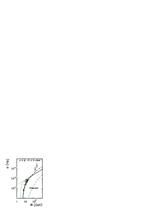
Figure 1: The cross section for $\gamma+p\rightarrow c\bar{c}X$ as a function of center-of-mass photon-proton energy. The dotted line is the result obtained with the Saturation Model, the dashed line includes kinematical threshold and the solid line includes in addition a suppression by the factor $(1-x_{c})^{7}$. The thick dashed-dotted line was obtained in the collinear approximation and the thin dash-dotted line represents the LO VDM contribution.

In Fig.1 we show predictions of the SM for charm photoproduction. The dotted line represents calculations based on Eq.(1). The result of this calculation exceeds considerably the fixed target experimental data [7, 8, 9, 10, 11, 12]. One should remember, however, that the simple formula (1) applies at high energies only. At lower energies one should include effects due to kinematical threshold. In the momentum representation this can be done by requiring: $M_{Q\bar{Q}}<W$, where $M_{Q\bar{Q}}$ is invariant mass of the final $Q\bar{Q}$ system. This cannot be done strictly in the mixed representation used to formulate the Saturation Model as here the information about heavy quark/antiquark momenta is not available. An approximate way to include the obvious limitation for heavy quark production is to neglect momenta and include only heavy quark masses in calculating $M_{Q\bar{Q}}$. This upper limit still exceeds the low energy experimental data. There are phase space limitations in the region $x_{g}\rightarrow$ 1 which has been neglected so far. Those can be estimated using naive counting rules. Counting reaction spectators we get for our process an extra correction factor

$$S_{sup}=(1-x_{g})^{7}\;.$$ (4)

In our case of mixed representation we are forced to use rather $x_{Q}$ instead of $x_{g}$. Such a procedure leads to a reasonable agreement with the fixed target experimental data as can be seen by comparing the solid line and the experimental data points.

The deviation of the solid line from the dotted line gives an idea of the range of the safe applicability of the Saturation Model for the production of the charm quarks/antiquarks. The cross section for $W>$ 20 GeV is practically independent of the approximate treatment of the threshold effects. The only data in this region come from HERA. Here the Saturation Model seems to slightly underestimate the H1 collaboration data [13].

For comparison in Fig. 1 we show the result of similar calculations in the collinear approach (thick dash-dotted line). In this approach the cross section reads as

$$\sigma_{\gamma N\rightarrow Q\bar{Q}}(W)=\int dx_{N}\;g_{N}(x_{N},\mu_{F}^{2})\;\sigma_{\gamma g\rightarrow Q\bar{Q}}(\hat{W})\;,$$ (5)

where $\hat{W}$ is energy in the $\gamma g$ system. The gluon distribution in the nucleon is taken from Ref.[16]. In the calculation shown in Fig.1 we have taken $\mu_{F}^{2}=\mu_{R}^{2}=m_{Q}^{2}+p_{\perp}^{2}$ with $p_{\perp}$ being the heavy quark/antiquark transverse momentum. The traditional collinear approach gives steeper energy dependence in the energy region considered than the SM prodictions. In order to test both approaches more, experimental data for different energies $W>$ 20 GeV are needed.

The calculation above is not complete. For real photons a soft vector dominance contribution due to photon fluctuation into vector mesons should be included on the top of the dipole contribution considered up to now. The VDM component seems unavoidable in order to understand the behaviour of $F_{2}^{p}-F_{2}^{n}$ at small photon virtualities [18]. Furthermore it seems rather a natural explanation of the strong virtuality dependence of the structure function of the virtual photon as measured recently [19].

In the present calculation we include only dominant gluon-gluon fusion component. In this approximation

$$\sigma_{\gamma N\rightarrow Q\bar{Q}}^{VDM}(W)=\sum_{V}\frac{4\pi}{f_{V}^{2}}\;\int dx_{V}dx_{N}\;g_{V}(x_{V},\mu^{2}_{F})\;g_{N}(x_{N},\mu^{2}_{F})\;\sigma_{gg\rightarrow Q\bar{Q}}(\hat{W})\;.$$ (6)

Here the $f_{V}$ constants describe the transition of the photon into vector mesons ($\rho$, $\omega$, $\phi$) and are taken in the on-shell approximation from the decay of vector mesons into dilepton pairs [18] taking into account finite width corrections. The gluon distributions in vector mesons are taken as that for the pion [15]

$$g_{V}(x_{V},\mu_{F}^{2})=g_{\pi}(x_{\pi},\mu_{F}^{2})$$ (7)

and that in the nucleon from Ref.[16]. For factorization scale we take $\mu_{F}^{2}=m_{Q}^{2}+p_{\perp}^{2}$ with $p_{\perp}$ being the heavy quark/antiquark transverse momentum. The dash-dotted line in Fig.1 shows the VDM contribution calculated in the leading order (LO) approximation for $\sigma_{gg\rightarrow Q\bar{Q}}$ (see e.g.[17]). The so-calculated VDM contribution cannot be neglected at high energies. Taking into account that usually the next-to-leading order approximation leads to an enhancement by a factor $K\sim$ 2, the VDM contribution is as important as the continuum calculated above.

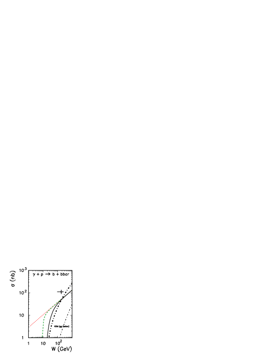
Figure 2: The cross section for $\gamma+p\rightarrow b\bar{b}X$ as a function of the center-of-mass photon-proton energy. The meaning of the curves is the same as in the previous figure. The experimental data point is from [14].

The situation for bottom photoproduction seems similar. In Fig.2 we compare the Saturation Model predictions with the data from the H1 collaboration [14]. Here the threshold effects may survive up to very high energy $W\sim$ 50 GeV. Again the predictions of the Saturation Model are slightly below the H1 experimental data point. The relative magnitude of the VDM component is similar as for the charm production.

The Saturation Model slightly underestimates high-energy data for both charm and bottom production. The parameters of the Saturation Model: $\sigma_{0}$ and $m_{eff}$ are to some extend correlated when extracted from the fit to the experimental data. In principle, because in the case of heavy quark production one is free of the uncertainty of the effective quark mass, one could allow to modify $\sigma_{0}$ to describe the HERA data on heavy quark production. It is obvious that then one would need to increase $m_{eff}$ to describe $\sigma_{\gamma N}^{tot}$. We shall leave this option for a separate study.

3 Heavy quark production in photon-photon scattering

3.1 Heavy quark-antiquark pair production

In the dipole-dipole approach (see for instance [3]) the total cross section for $\gamma\gamma\rightarrow Q\bar{Q}$ production can be expressed as

$$\sigma_{\gamma\gamma\rightarrow Q\bar{Q}}^{dd}(W) = \sum_{f_{2}\neq Q}\int|\Phi^{Q\bar{Q}}(\rho_{1},z_{1})|^{2}|\Phi^{f_{2}\bar{f}_{2}}(\rho_{2},z_{2})|^{2}\sigma_{dd}(\rho_{1},\rho_{2},x_{Qf})\;d^{2}\rho_{1}dz_{1}d^{2}\rho_{2}dz_{2}$$

$$+ \sum_{f_{1}\neq Q}\int|\Phi^{f_{1}\bar{f}_{1}}(\rho_{1},z_{1})|^{2}|\Phi^{Q\bar{Q}}(\rho_{2},z_{2})|^{2}\sigma_{dd}(\rho_{1},\rho_{2},x_{fQ})\;d^{2}\rho_{1}dz_{1}d^{2}\rho_{2}dz_{2}\;,$$

where $\Phi^{q\bar{q}}$ are the quark-antiquark wave functions of the photon in the mixed representation and $\sigma_{dd}$ is dipole-dipole cross section. While for the heavy quark-antiquark pair the photon wave function is well defined, for light quarks one usually takes the perturbatively calculated wave function with the quark/antiquark mass replaced by $m_{eff}$. This parameter provides a useful cut-off of large-size configurations in the photon wave function.

There are two problems associated with direct use of (LABEL:SM_QQbar). First of all, it is not completely clear how to generalize the dipole-dipole cross section from the dipole-nucleon cross section parametrized in [1]. Secondly, formula (LABEL:SM_QQbar) is correct only at sufficiently high energy $W\gg 2m_{Q}$. At lower energies one should worry about proximity of the kinematical threshold.

In a very recent paper [3] a new phenomenological parametrization for the azimuthal angle averaged dipole-dipole cross section has been proposed:

$$\sigma_{dd}^{a,b}(x_{ab},\rho_{1},\rho_{2})=\sigma_{0}^{a,b}\left[1-\exp\left(-\frac{r_{eff}^{2}}{4R_{0}^{2}(x_{ab})}\right)\right]\;.$$ (9)

Here

$$R_{0}(x_{ab})=\frac{1}{Q_{0}}\left(\frac{x_{ab}}{x_{0}}\right)^{-\lambda/2}$$ (10)

and the parameter $x_{ab}$ which controls the energy dependence was defined as

$$x_{ab}=\frac{4m_{a}^{2}+4m_{b}^{2}}{W^{2}}\;.$$ (11)

In order to take into account threshold effects for the produtcion of $q\bar{q}q^{\prime}\bar{q}^{\prime}$ an extra phenomenological function has been introduced [3]

$$S_{thresh}(x_{ab})=(1-x_{ab})^{5}$$ (12)

which is put to zero if $x_{ab}>1$. This factor strongly reduces the cross section at low energies. Different prescriptions for $r_{eff}$ have been considered in [3], with $r_{eff}^{2}=\frac{\rho_{1}^{2}\rho_{2}^{2}}{\rho_{1}^{2}+\rho_{2}^{2}}$ being the best choice phenomenologically [3].

The phenomenological threshold factor (12) does not guarantee automatic vanishing of the cross section exactly below the true kinematical threshold $W=2m_{a}+2m_{b}$. Therefore instead of the phenomenological factor we rather impose an extra kinematical constraint: $M_{f\bar{f}}+M_{Q\bar{Q}}<W$ on the integration in (LABEL:SM_QQbar). The use of extra dynamical factor $(1-x_{ab})^{5}$ for heavy quark production in photon-photon collisions is in our opinion disputable. Instead, in the present paper we shall estimate the effect of damping of the cross section in the neighbourhood of threshold due to simple kinematical limitations on the final quark/antiquark transverse momenta. As will be discussed in the course of this paper this leads to a similar suppression at least numerically.

Identically as for $\gamma N$ scattering in the mixed representation, where the transverse momenta are not given explicitly, the quark-antiquark invariant mass is not well defined. We suggest therefore to use rather the effective (z-dependent!) invariant masses $<M_{q\bar{q}}>$ with transverse momenta neglected and effective quark mass as used in many other mixed representation calculations for $\gamma N$ scattering known in the literature. It is not completely clear how to generalize the energy dependence of $\sigma_{dN}$ in photon-nucleon scattering to the energy dependence in $\sigma_{dd}$ in photon-photon scattering. In the following we define the parameter which controls the Saturation Model energy dependence of the dipole-dipole cross section in a symmetric way as

$$x_{Qf} = x_{Qf}(z_{1},z_{2})=C\cdot(<M_{Q\bar{Q}}>(z_{1})+<M_{f\bar{f}}>(z_{2}))^{2}/W^{2}\;,$$

$$x_{fQ} = x_{fQ}(z_{1},z_{2})=C\cdot(<M_{f\bar{f}}>(z_{1})+<M_{Q\bar{Q}}>(z_{2}))^{2}/W^{2}$$ (13)

instead of (11). Here we have made explicit the dependence on $z_{1}$ and $z_{2}$. In the following we shall use C = 1 and only in some cases compare to the results with C = 0.5. In Fig.3 we compare our prescription with those used in [3] for the $c\bar{c}$ production (left panel) and for the $b\bar{b}$ production (right panel). In comparison to [3] our prescription leads to a small reduction of the cross section far from the threshold and a significant enhancement close to the threshold. Some consequences of this will be discussed separately in the context of the observed excess of $b\bar{b}$ production in positron-electron collisions.

For comparison we show in Fig.3 also a result obtained in the two-gluon exchange model. In this case

$$\sigma_{dd}(\vec{\rho}_{1},\vec{\rho}_{2})=\frac{8}{9}\int\frac{d^{2}\kappa}{\kappa^{4}}\alpha_{s}^{2}(\mu^{2})\cdot(2-e^{i\vec{\kappa}\vec{\rho}_{1}}-e^{-i\vec{\kappa}\vec{\rho}_{1}})\cdot(2-e^{i\vec{\kappa}\vec{\rho}_{2}}-e^{-i\vec{\kappa}\vec{\rho}_{2}})\;.$$ (14)

In principle one can allow for running of $\alpha_{s}(\mu^{2})$. However, the choice of the scale $\mu^{2}$ is not completely clear. In the present calculation a rather large constant value $\alpha_{s}$ = 0.35 was taken. If $\alpha_{s}(m_{c}^{2}/m_{b}^{2})$ was used the cross section would be negligibly small. Thus it becomes clear that the Saturation Model leads to a huge enhancement relative to the two-gluon exchange model high above the threshold. Close to the threshold both results almost coincide. The departure of the 2g-exchange result from the constant value below $W\approx 3\cdot(2m_{Q})$ is due to the threshold effects.

In calculating the main SM component above we have considered only obvious kinematical limitations possible to implement in the mixed representation. As already discussed it is not possible to include the transverse momentum limitations in the mixed representation. Now we shall estimate the effect due to the kinematically limited integration over transverse momenta of final heavy quarks/antiquarks. This effect can be taken into account consistently only in the momentum representation. This would require a reformulation of the whole Saturation Model and clearly goes beyond the scope of the present analysis. In order to gain experience we have studied first the effect of the kinematical constraint on the transverse momenta in the two-gluon exchange approximation in the momentum representation. In this case we can easily both include and exclude the kinematical limitations on transverse momenta. Then one can approximately correct our mixed representation calculation as

$$\sigma_{\gamma\gamma\rightarrow Q\bar{Q}}^{mixed}(W)|_{corr}=\sigma_{\gamma\gamma\rightarrow Q\bar{Q}}^{mixed}(W)|_{approx}\cdot R_{c/a}(W)\;.$$ (15)

Here for brevity we have introduced the ratio:

$$R_{c/a}(W)=\frac{\sigma_{\gamma\gamma\rightarrow Q\bar{Q}}^{2g,mom}(W)|_{corr}}{\sigma_{\gamma\gamma\rightarrow Q\bar{Q}}^{2g,mom}(W)|_{approx}}\;.$$ (16)

In Fig.4 we show the so-obtained correction factor as a function of W for both $c\bar{c}$ (solid) and $b\bar{b}$ (dashed) production. As can be seen from the figure the correction is significant even far from the threshold, i.e. leads to a significant damping of the cross section. We shall discuss this damping in the context of the $b\bar{b}$ deficit in a separate section.

3.2 $2Q2\bar{Q}$ final states

The dipole-dipole approach in general, and the Saturation Model as its particular realization, leads to a unique prediction for the $2Q2\bar{Q}$ (two identical heavy quarks and two identical heavy antiquarks) production in the final state

$$\sigma_{\gamma\gamma\rightarrow 2Q2\bar{Q}}^{dd}(W)=\int|\Phi_{1}^{Q\bar{Q}}(\rho_{1},z_{1})|^{2}|\Phi_{2}^{Q\bar{Q}}(\rho_{2},z_{2})|^{2}\sigma_{dd}(\rho_{1},\rho_{2},x_{QQ})\;d^{2}\rho_{1}dz_{1}d^{2}\rho_{2}dz_{2}\;.$$ (17)

The same prescriptions are used here as for the $Q\bar{Q}$ final states in the previous section.

In Fig.5 we compare our prescription to that from [3] for four heavy quark production for Q=c (left panel) and for Q=b (right panel). Here there is even larger difference between the two prescriptions than for the heavy quark-antiquark pair production. In Fig.6 we show the ratio defined as

$$R_{4/2}(W)\equiv\frac{\sigma_{\gamma\gamma\rightarrow 2Q2\bar{Q}}(W)}{\sigma_{\gamma\gamma\rightarrow Q\bar{Q}}(W)}\;.$$ (18)

Sufficiently above the kinematical threshold $W\gg 4m_{Q}$ the ratio saturates at the level of about 8 % and 1 % for $2c2\bar{c}$ and $2b2\bar{b}$, respectively. The fluctuations of the order of 1 % that one can observe in the figure are of numerical origin.

The predictions for $\gamma\gamma\rightarrow 2Q2\bar{Q}$ shown in Fig.5 and 6 are the only ones in the literature we know. In the standard collinear approaches the $2Q2\bar{Q}$ final states can be produced only in next-to-leading order calculations or/and in the hadronization process, if the charmed mesons, e.g. $D^{*}$, are measured to identify charm quarks/antiquarks. It would be interesting to compare in the future the present result with the standard collinear NLO predictions. Also from the experimental side the $2Q2\bar{Q}$ production in photon-photon collisions is terra incognita. In our opinion, the $2Q2\bar{Q}$ channel has a better chance to be a stringent test of the dipole-dipole approaches and the Saturation Model in particular. It is not clear to us if the experimental verification can be feasible with the present LEP2 statistics. It seems, however, possible with the future photon-photon colliders like that planned at TESLA (see for instance [6]).

3.3 Short- versus long-distance phenomena

What are typical distances probed in heavy quark production ? Is the heavy quark production a short distance phenomenon ? These questions can be easily answered in the mixed representation formulation considered in the present paper. In Fig.7 we display the integrand of

$$\sigma_{\gamma\gamma\rightarrow c\bar{c}}(W)=\int\;I(\rho_{1},\rho_{2})\;d\rho_{1}d\rho_{2}\;.$$ (19)

The maxima in Fig.7 correspond to the most probable situations. For one light ($m_{u}$ = $m_{d}$ = $m_{0}$, $m_{s}$ = $m_{0}$ + 0.15 GeV) and second heavy quark-antiquark pair the map is clearly asymmetric. One can observe a ridge parallel to the $\rho_{1}$ or $\rho_{2}$ axis. There is not well localized maximum. Both short and long distances are probed.

For comparison, in the bottom part of the figure, we show similar maps when both pairs consist of light (u,d,s) quarks/antiquarks (left-bottom) and in the case when both pairs consist of charm quarks/antiquarks (right-bottom). For light quarks (u,d,s) one observes a clear maximum at $(\rho_{1},\rho_{2})$ = (1 GeV^-1, 1 GeV^-1) = (0.2 fm, 0.2 fm). In this case a nonnegligible strength extends, however, up to large distances $\rho_{1}$ and $\rho_{2}$. Only in the case of the production of two $c\bar{c}$ pairs the cross section is dominated exclusively by short-distance phenomena.

3.4 Hadronic single-resolved processes

Up to now we have calculated the contribution when photons fluctuate into quark-antiquark pairs. Then the final quark and antiquark carry away the whole longitudinal momentum of the parent photon and are predominantly emitted in the same photon hemisphere. In the standard collinear approach one usually includes so-called resolved contributions, when heavy quark-antiquark pairs are created either in the photon-gluon / gluon-photon fusion or in the gluon-gluon fusion and quark-antiquark annihilation processes. In the first case, known as the single-resolved process, only a small fraction of the first or the second photon longitudinal momentum enters into the production of heavy quark or antiquark. In the second case, known as double-resolved process, this is true for both photons. The arguments above demonstrate that the resolved processes are different, at least kinematically, from those included in the Saturation Model, or more generally in the dipole-dipole interaction picture. This means that the resolved processes are not included in the dipole-dipole scattering approach. At the same time the standard collinear approach is not complete too. Can the dipole approach be supplemented to include the hadronic resolved processes? Let us try to answer this question by combining a simple vector dominance model and the dipole picture. For simplicity we shall limit to the dominant photon fluctuations into light vector mesons: $\rho$, $\omega$ and $\phi$, only. It is sufficient to include the light vector mesons because the contribution of heavier mesons, as being highly off-mass-shell, is expected to be considerably suppressed.

If the first photon fluctuates into the vector mesons the so-defined single-resolved contribution to the heavy quark-antiquark production can be calculated analogically to the photon-nucleon case as

$$\sigma^{SR,1}_{\gamma\gamma\rightarrow Q\bar{Q}}(W)=\sum_{V_{1}}\frac{4\pi}{f_{V_{1}}^{2}}\int|\Phi_{2}^{Q\bar{Q}}(\rho_{2},z_{2})|^{2}\sigma_{V_{1}d}(\rho_{2},x_{1})\;d^{2}\rho_{2}dz_{2}\;,$$ (20)

where $\Phi_{2}^{Q\bar{Q}}$ is the second photon $Q\bar{Q}$ wave function and $\sigma_{V_{1}d}$ is vector meson - dipole total cross section. In the spirit of the Saturation Model, we shall parametrize the latter exactly as for the photon-nucleon case [1] with a simple rescaling of the normalization factor $\sigma_{0}^{dV}=2/3\cdot\sigma_{0}^{dN}$. In the present calculation $\sigma_{0}^{dN}$ as well as the other parameters of SM are taken from [1]. Fully analogically if the second photon fluctuates into vector mesons

$$\sigma^{SR,2}_{\gamma\gamma\rightarrow Q\bar{Q}}(W)=\sum_{V_{2}}\frac{4\pi}{f_{V_{2}}^{2}}\int|\Phi_{1}^{Q\bar{Q}}(\rho_{1},z_{1})|^{2}\sigma_{dV_{2}}(\rho_{1},x_{2})\;d^{2}\rho_{1}dz_{1}\;.$$ (21)

This clearly doubles the first contribution (20) to the total cross section. Of course, if the rapidity distributions of heavy quark/antiquark are considered, both contributions must be treated independently. We leave the analysis of $(\eta,k_{\perp})$ distributions for a separate study. The integrations in (20) and (21) are not free of kinematical constraints. When calculating both single-resolved contributions it should be checked additionally if the heavy quark-antiquark invariant mass $M_{Q\bar{Q}}$ is smaller than the total photon-photon energy $W$. As in the previous cases in the mixed representation it can be done only approximately. In analogy to $\gamma N$ scattering the most logical definition of the parameter which controls energy dependence of $\sigma_{V_{1}d}$ or $\sigma_{dV_{2}}$ is: $x_{2/1}=M_{Q\bar{Q}}^{2}(z_{2/1})/W^{2}$ and corresponds to the gluon momentum fraction in the second or first photon (vector meson), respectively.

In Fig.8 we compare the present result with the result of the leading order collinear approximation. In the latter case

$$\sigma_{\gamma\gamma\rightarrow Q\bar{Q}}^{SR,coll} = \sum_{V_{1}}\frac{4\pi}{f_{V_{1}}^{2}}\;\int\;g_{V_{1}}(x_{V_{1}},\mu_{F}^{2})\;\sigma_{g\gamma\rightarrow Q\bar{Q}}\;dx_{V_{1}}$$ (22)

$$+ \sum_{V_{2}}\frac{4\pi}{f_{V_{2}}^{2}}\;\int\;g_{V_{2}}(x_{V_{2}},\mu_{F}^{2})\;\sigma_{\gamma g\rightarrow Q\bar{Q}}\;dx_{V_{2}}\;.$$

Also in this calculation the gluon distributions in the vector mesons are taken as that for the pion [15] $g_{V}(x_{g},\mu_{F}^{2})=g_{\pi}(x_{g},\mu_{F}^{2})$. The scale $\mu_{F}^{2}=m_{c}^{2}+p_{\perp}^{2}$ is taken in practical calculation with $p_{\perp}$ being the transverse momentum of the final heavy quark.

There is a difference in shape of the cross section as obtained in the SM (thin solid) and collinear (dashed) approaches. Part of the difference may come from the fact that up to now we have not included phase space limitations when $x_{1/2}\rightarrow$ 1 which may be important at low energies. In this case a naive application of counting rules would lead to the following suppression factor

$$S_{SR}=(1-x_{1/2})^{2n_{SR}-1}\;.$$ (23)

Following standard prescription by making use of the picture that the unresolved photon probes the resolved one and assuming that a vector meson consists of a valence quark and antiquark we get $n_{SR}=3$. The SM result corrected by (23) is shown by the thick solid line in Fig.8. After the correction the results obtained from the two different approaches are numerically fairly similar.

3.5 Summing all contributions to inclusive cross section

In Fig.9 we show different contributions to the inclusive $c/\bar{c}$ (left panel) and $b/\bar{b}$ (right panel) production in photon-photon scattering. The thick solid line represents the sum of all contributions.

Let us start from the discussion of the inclusive charm production. The experimental data of the L3 collaboration [20] are shown for comparison. The modifications discussed above lead to a small damping of the cross section in comparison to [3]. The corresponding result (long-dashed line) stays below the recent experimental data of the L3 collaboration [20]. The considered in the present paper hadronic single-resolved contribution constitutes about 30 - 40 % of the main Saturation Model contribution. At high energies the cross section for the $2c2\bar{c}$ component is about 8 % of that for the single $c\bar{c}$ pair component (see Fig.5). In inclusive cross section its contribution should be doubled because each of the heavy quarks/antiquarks can be potentially identified experimentally. In principle the events with $2c2\bar{c}$ can be subtracted both when flavour tagging is applied or charmed mesons are measured to identify $c$ or $\bar{c}$. In practice, because the efficiency of the flavour tagging is very small and only a small fraction of $2c2\bar{c}$ can be removed, the measured inclusive cross section is two times bigger than the integrated cross section to the $2c2\bar{c}$ final state.

At higher photon-photon energies the direct contribution is practically negligible. This is in contrast to the energy dependence in the positron-electron collisions. Here even at large energies the direct contribution constitutes almost half of the corresponding cross section. The reason is that even at high $e^{+}e^{-}$ energies the contributions of small photon-photon energies are dominant which can be easily understood in the equivalent photon approximation to be discussed in the next section. The hadronic double-resolved contribution, when each of the two photons fluctuates into a vector meson, calculated as

$$\sigma_{\gamma\gamma\rightarrow Q\bar{Q}}^{DR,coll}=\sum_{V_{1},V_{2}}\frac{4\pi}{f_{V_{1}}^{2}}\frac{4\pi}{f_{V_{2}}^{2}}\int g_{V_{1}}(x_{V_{1}},\mu_{F}^{2})\;g_{V_{2}}(x_{V_{2}},\mu_{F}^{2})\;\sigma_{gg\rightarrow Q\bar{Q}}(\hat{W})\;dx_{V_{1}}dx_{V_{2}}$$ (24)

and shown by the thin solid line in the figure becomes important only at very high energies relevant for TESLA. Here we have consistently taken $g_{V}(x_{V},\mu_{F}^{2})=g_{\pi}(x_{V},\mu_{F}^{2})$ and $\mu_{F}^{2}=m_{Q}^{2}+p_{\perp}^{2}$.

The situation for bottom production (see right panel) is somewhat different. Here the main SM component is dominant. Due to smaller charge of the bottom quark than that for the charm quark the direct component is effectively reduced with respect to the dominant SM component by the corresponding ratio of quark/antiquark charges: $(1/9)^{2}:(4/9)^{2}=1/16$. The same is true for the $2b2\bar{b}$ component. Here in addition there are threshold effects which play a role up to relatively high energy. Also the single-resolved component is relatively smaller which has no simple explanation.

The role of different mechanisms for charm and bottom production is also summarized numerically in Table 1, where we have collected corresponding cross sections for a few selected values of photon-photon energies.

3.6 $e^{+}e^{-}\rightarrow e^{+}e^{-}b\bar{b}X$

Up to now no attempt was done to unfold experimentally the cross section for $\gamma\gamma\rightarrow b\bar{b}X$. Only cross section for the $e^{+}e^{-}\rightarrow b\bar{b}X$ reaction was obtained recently by the L3 and OPAL collaborations at LEP2 [20, 22]. The measured, both positron and electron antitagged, cross sections can not be described as a sum of direct and single-resolved contributions, even if next-to-leading order corrections are included [22]. The measured cross section exceeds the theoretical predictions by a large factor. This is a new situation in comparison to the charm production where the deficit is much smaller. We shall consider the case of bottom production in more detail below.

The cross section for the $e^{+}e^{-}\rightarrow b\bar{b}\;X$ reaction when both positron and electron are antitagged can be easily estimated in the equivalent photon approximation (EPA) as

$$\sigma(e^{+}e^{-}\rightarrow b\bar{b}X;W_{ee})=\int dx_{A}dx_{B}\;f_{A}(E_{b},\theta_{max},x_{A})f_{B}(E_{b},\theta_{max},x_{B})$$

$$\sigma(\gamma\gamma\rightarrow b\bar{b}X;W)\;,$$ (25)

where $f_{A}$ and $f_{B}$ are virtuality-integrated flux factors of photons in the positron and electron, respectively, and $\theta_{max}$ is the maximal angle of the positron/electron not to be identified by the experimental aparatus. In the present analysis we calculate the integrated flux factors $f_{A}$ and $f_{B}$ in a simple logarithmic approximation. The photon-photon energy can be calculated in terms of photon longitudinal momentum fractions $x_{A}$ and $x_{B}$ in positron and electron, respectively, as $W=\sqrt{x_{A}x_{B}s_{ee}}$. It is instructive to visualize how different regions of $W_{\gamma\gamma}$ contribute to $\sigma(e^{+}e^{-}\rightarrow b\bar{b}X;W_{ee})$. For this purpose it is useful to transform variables from $x_{A},x_{B}$ to $x_{F}\equiv x_{A}-x_{B}$ and $W_{\gamma\gamma}=W$. Then

$$\sigma(e^{+}e^{-}\rightarrow b\bar{b}X;W_{ee})=\int dx_{F}dW\;{\cal J}\;f_{A}(E_{b},\theta_{max},x_{A})f_{B}(E_{b},\theta_{max},x_{B})$$

$$\sigma(\gamma\gamma\rightarrow b\bar{b}X;W)\;,$$ (26)

where the jacobian ${\cal J}$ is a simple function of kinematical variables.

Before we go to the $b\bar{b}$ production let us look at the corresponding $c\bar{c}$ production. In Fig.10 we compare the $x_{F}$-integrated cross section $d\sigma/dW(e^{+}e^{-}\rightarrow c\bar{c}X)$ with recent experimental data of the L3 collaboration [20]. Different mechanisms are shown separately. The agreement with the L3 collaboration experimental data here is even better than for the unfolded $\gamma\gamma\rightarrow c\bar{c}$ data shown in Fig.9. This is probably due to our simplified treatment of the photon flux factors. The good agreement of the sum of all contributions with the data gives credit to our model calculations.

The integrand $I(x_{F},W)$ of (26) for $b\bar{b}$ is shown in Fig.11 for the direct production (left panel) and for the Saturation Model (right panel) including all contributions considered in the present analysis. Quite different pattern can be observed for both mechanisms. While for the direct production one is sensitive mainly to low-energy photon-photon collisions, in the Saturation Model the contributions of high-energies can not be neglected and one has to integrate over $W_{\gamma\gamma}$ essentially up to $W_{ee}$. This difference in $W_{\gamma\gamma}$ is due to different energy dependence of $\sigma(\gamma\gamma\rightarrow b\bar{b};W_{\gamma\gamma})$ for the different mechanisms considered as has been discussed above. But even in the latter case the integrated cross section is very sensitive to the region of not too high-energies $W\sim$ 20 GeV, where the not fully understood threshold effects may play essential role.

For LEP2 averaged energy $<W_{ee}>\approx$ 190 GeV the cross section integrated taking into account experimental cuts is $\sigma(e^{+}e^{-}\rightarrow b\bar{b}X)$ = 6.1 pb (C = 1) or 7.4 pb (C = 1/2) for the dipole-dipole SM scattering process. If the limitations on transverse momenta are included in addition through the factor $R_{c/a}$ (see (16)), then the corresponding cross section is reduced to 3.2 pb (C = 1) or 3.9 pb (C = 1/2). Corresponding cross section for the direct production is $\sigma(e^{+}e^{-}\rightarrow b\bar{b}X)$ = 1.2 pb. The hadronic single-resolved contribution calculated here in the Saturation Model as described in the present paper is very similar in size to that calculated in the standard collinear approach [22]. As can be seen in Table 2 the $2b2\bar{b}$ contribution is practically negligible. We have completely omitted the double-resolved contribution which is practically negligible (see Table 1). The sum of the direct, $b\bar{b}$ SM, $2b2\bar{b}$ SM and the hadronic single resolved SM component is 9.3-10.6 pb in the case when no transverse momenta cuts on the main SM component are included and 6.4-7.1 pb with the cuts. These numbers should be compared to experimentally measured $\sigma(e^{+}e^{-}\rightarrow b\bar{b}X)$ = 13.1 $\pm$ 2.0 (stat) $\pm$ 2.4 (syst) pb [23] (L3) and preliminary $\sigma(e^{+}e^{-}\rightarrow b\bar{b}X)$ = 14.2 $\pm$ 2.5 (stat) $\pm$ 5.0 (syst) pb [23] (OPAL). In comparison to earlier calculations in the literature, the theoretical deficit is much smaller. The success of the present calculation relies on the inclusion of a few mechanisms neglected so far, in particular the dipole-dipole contribution which, in our opinion, is not contained in the standard collinear approach.

Up to now only $W_{\gamma\gamma}$-integrated cross section has been determined experimentally. This, in fact, does not allow to identify experimentally whether the problem is in low or high $W_{\gamma\gamma}$. In order to identify better the region where the standard collinear approach fails it would be useful to bin the experimental cross section in the intervals of $W_{\gamma\gamma}$ making use of a possibility to measure $W_{vis}$ which can be related to $W_{\gamma\gamma}$ via a suitable Monte Carlo program. At present, even splitting the cross section for $e^{+}e^{-}\rightarrow b\bar{b}X$ into $\sigma(W_{\gamma\gamma}<W_{0})$ and $\sigma(W_{\gamma\gamma}>W_{0})$ for $W_{0}\sim$ 20 GeV would be useful and should shed more light on the problem of the experimental excess of $b\bar{b}$ relative to the “standard” QCD approach.

3.7 Subasymptotic components to the dipole-dipole approach to $\gamma\gamma\rightarrow Q\bar{Q}$

The Saturation Model by construction includes only dominant asymptotic contributions relevant at very high energies. As discussed above the problem of heavy quark production (especially $b\bar{b}$) may be a bit more complicated. In the following we shall try to generalize the dipole-dipole approach to include dynamics which may be of relevance also close to threshold. As discussed above this can be the region of the deficit of theoretical predictions observed for the bottom production in photon-photon collisions.

In the following as an example we shall try to estimate the cross section for the process when the quark associated with one photon annihilates with the same-flavour antiquark associated with the second photon. Then the heavy quark-antiquark pair can be produced via exchange of s-channel gluon. In the dipole-dipole approach this effect can be estimated(!) in terms of the familiar quark-antiquark photon wave functions as follows

$$\sigma_{\gamma\gamma\rightarrow Q\bar{Q}}^{sub} = \sum_{f_{1},f_{2}}\delta_{f_{1}f_{2}}\int dz_{1}d^{2}\rho_{1}dz_{2}d^{2}\rho_{2}\;|\Psi^{f_{1}\bar{f}_{1}}(z_{1},\rho_{1})|^{2}|\Psi^{f_{2}\bar{f}_{2}}(z_{2},\rho_{2})|^{2}$$ (27)

$$\cdot [\sigma_{q\bar{q}\rightarrow Q\bar{Q}}(\hat{s},\vec{\rho}_{1},\vec{\rho}_{2})+\sigma_{\bar{q}q\rightarrow Q\bar{Q}}(\hat{s},\vec{\rho}_{1},\vec{\rho}_{2})]\;.$$

The Kronecker $\delta$ reflects flavour conservation in QCD. In the following we shall include only light flavours (u,d,s) as “constituents” of both photons and use the same treatment (suppression) of large size physics as in all cases before. For the purpose of the estimate a sensible approximation is to neglect light quark/antiquark transverse momenta and write

$$\sigma_{\gamma\gamma\rightarrow Q\bar{Q}}^{sub} = \sum_{f}\int\;q_{f/\gamma_{1}}^{eff}(z_{1})\;\bar{q}_{f/\gamma_{2}}^{eff}(z_{2})\;\sigma_{q\bar{q}\rightarrow Q\bar{Q}}(\hat{s})\;dz_{1}dz_{2}$$ (28)

$$+ \sum_{f}\int\;\bar{q}_{f/\gamma_{1}}^{eff}(z_{1})\;q_{f/\gamma_{2}}^{eff}(z_{2})\;\sigma_{\bar{q}q\rightarrow Q\bar{Q}}(\hat{s})\;dz_{1}dz_{2}\;,$$

where $\sigma_{q\bar{q}\rightarrow Q\bar{Q}}$ or $\sigma_{\bar{q}q\rightarrow Q\bar{Q}}$ are calculated in the Born approximation with collinear incoming light quark and antiquark [17]. The argument of $\alpha_{s}(\mu_{R}^{2})$ is set to $\mu_{R}^{2}=\hat{s}$ in practical calculations. In Eq.(28) we have introduced for brevity

$$q_{f}^{eff}(z)\equiv\int|\Psi^{f\bar{f}}(z,\rho)|^{2}\;d^{2}\rho\;.$$ (29)

Because the perturbative photon wave function is singular at $\rho$ = 0, the expression above is formally divergent. However, there is a natural cut-off at small $\rho$’s: $\rho_{min}\sim 1./\sqrt{\hat{s}}$ which makes the integral finite. This cut-off corresponds to the upper limit on transverse momenta in the momentum representation calculations.

In Fig.12 we show the cross section for the subasymptotic contribution considered for both $c\bar{c}$ and $b\bar{b}$ production. The maximum of the cross section is concentrated in the close neighbourood of corresponding kinematical thresholds at $W\sim$ 10 GeV and $W\sim$ 30 GeV for charm and bottom, respectively. This concentration of the strenght at threshold justifies the introduced name “subasymptotic” for the process considered. The main (asymptotic) component of SM is shown for comparison by the dashed line and the QPM contribution by the dotted line. The subasymptotic contribution considered shows similar energy dependence as the QPM component. At high energies it is rather small in comparison to the leading asymptotic component. Only, at threshold it constitutes a nonnegligible fraction of the heavy quark production cross section. When integrating $\sigma_{\gamma\gamma\rightarrow b\bar{b}X}^{sub}$ with virtual photon flux factors over $W_{\gamma\gamma}$ and $x_{F}$ we obtain $\sigma_{e^{+}e^{-}\rightarrow b\bar{b}X}^{sub}\approx$ 0.1 pb at $W_{ee}$ = 190 GeV. This is rather a conservative estimate because in the present calculations we have used leading order formulas for $\sigma_{q\bar{q}\rightarrow Q\bar{Q}}$. This seems tiny in comparison to the contributions considered before (see Table 2). We could increase slightly the cross section by a different choice of the renormalization scale $\mu_{R}^{2}$ in calculating $\sigma_{q\bar{q}\rightarrow Q\bar{Q}}$. We expect that in reality $\sigma_{e^{+}e^{-}\rightarrow b\bar{X}}^{sub}$ should not exceed 0.5 pb.

3.8 Quark-antiquark correlations

So far mainly integrated cross section for heavy quark/antiquark production was considered in the literature. Only in a few cases inclusive distributions in transverse momentum or rapidity (see e.g.[24]) were presented. No attempts were done so far to analyze the final state in more detail. In our opinion investigating correlations between heavy quark - heavy antiquark could be much more conclusive to identify the production mechanisms than the integrated cross section or even a single variable distribution.

In principle any correlation between two kinematical variables of the final quark and antiquark would be of interest. We suggest that the following final quark/antiquark momentum fractions:

$$x_{Q}=\frac{\vec{p}_{Q}}{|\vec{p}_{Q}|}{\hat{n}}_{\gamma_{1}}\;,$$

$$x_{\bar{Q}}=\frac{\vec{p}_{\bar{Q}}}{|\vec{p}_{\bar{Q}}|}{\hat{n}}_{\gamma_{1}}\;,$$ (30)

where

$${\hat{n}_{\gamma_{1}}}=\frac{\vec{p}_{\gamma_{1}}}{|\vec{p}_{\gamma_{1}}|}$$ (31)

would be very useful to separate the different mechanisms (approches) analysed in the present paper. In the definition above $\vec{p}_{Q}$ and $\vec{p}_{\bar{Q}}$ are momenta of heavy quark and antiquark, respectively, and $\vec{p}_{\gamma_{1}}$ is the momentum of the first photon, all in the photon-photon center of mass frame. By definition -1 $<x_{Q},x_{\bar{Q}}<$ 1. Similar quantities are being used at present when analyzing e.g. jet production at HERA to separate out resolved and direct processes.

In Fig.13 we present a sketch of naive expectations. Although a precise map requires detailed calculations for each mechanism separately, which is beyond the scope of the present analysis, it is obvious that the separation of different mechanisms here should be much better then for any inclusive spectra. In the case of dipole-dipole approach (the elongated ellipses) this would require to go to the momentum representation. The mixed representation used in the present paper is useful only for integrated cross sections.

Experimentally, the suggested analysis would be difficult at LEP2 because of rather limited statistics. We hope that such an analysis will be possible at the photon-photon option at TESLA. At present, even localizing a few LEP2 coincidence $c\bar{c}$ events in the diagram $x_{c}$ versus $x_{\bar{c}}$ would be instructive.

4 Conclusions

There is no common consensus in the literature on detailed understanding of the dynamics of photon-nucleon and photon-photon collisions. In this article we have limited the discussion to the production of heavy quarks simultaneously in photon-nucleon and photon-photon collisions at high energies.

A special emphasis has been put on the application of the Saturation Model which turned out recently very succesfull in the description of experimental data for DIS at small Bjorken $x$. We have suggested how to generalize the model to applications with real photons. The sizeable mass of charm or bottom quarks sets natural low energy limit on naive application of the Saturation Model. Here a careful treatment of the kinematical threshold is required. In the mixed representation used to formulate the Saturation Model the effect can be included only approximately.

We have started the analysis from (real) photon-nucleon scattering, which is very close to the domain of the Saturation Model as formulated in [1]. If the kinematical threshold corrections are included the SM gives numerically similar results as the standard collinear approach for both charm and bottom production. We have numerically estimated the vector dominance contribution to the heavy quark production.

The major part of the present analysis has been devoted to real photon - real photon collisions. For the first time in the literature we have estimated the cross section for the production of $2c2\bar{c}$ final state. Furthermore we have discussed how to include this component to the inclusive charm production as derived in the present experimental analyses. We have found that this component constitutes up to 10-15 % of the inclusive charm production at high energies and is negligible for the bottom production. We have shown how to generalize the Saturation Model to the case when one of the photons fluctuates into light vector mesons. It was found that this component yields a significant correction of about 30-40 % for inclusive charm production and 15-20 % for bottom production. We have shown that the double resolved component, when both photons fluctuate into light vector mesons, is nonnegligible only at very high energies, both for the charm and bottom production.

We have shown that the production of $c\bar{c}$ pairs (the same is true for $b\bar{b}$) is not completely of perturbative character and involves both short- and large-size contributions. The latter as nonperturbative are unavoidably subjected to some modeling. Present experimental statistics do not allow to extract cross section for the $\gamma\gamma\rightarrow b\bar{b}$ reaction and therefore it is not clear where the observed deficit reside. It is not excluded that the apparent deficit of bottom quarks may reside at photon-photon energies close to threshold. This is a region where the underlying physics was never carefully studied. We have made a crude estimate of the subasymptotic quark-antiquark annihilation component to $\gamma\gamma\rightarrow b\bar{b}$. Although very small at high $W_{\gamma\gamma}$ its contribution to the $e^{+}e^{-}\rightarrow b\bar{b}$ reaction was found to be not completely negligible. Adding all contributions considered in the present analysis together removes a huge deficit observed in earlier works on $e^{+}e^{-}\rightarrow b\bar{b}X$.

The present analysis is based on the leading order impact factors. It would be desirable in the future to perform complete next-to-leading order calculation of heavy quark/antiquark production in the $k_{\perp}$-factorization approach. We expect that calculating photon impact factors consistently up to next-to-leading order [25] may be crucial for heavy quark production.

Finally we have discussed a possibility to distniguish experimentally the different mechanisms discussed in the present paper by measuring heavy quark - antiquark correlations. This suggestion requires, however, further detailed studies of the Monte Carlo type, including experimental possibilities and limitations.

Acknowledments I am indebted to Jan Kwieciński and Leszek Motyka for the discussion of their recent work [3] and Akos Csilling and Valerii Andreev for the discussion of the recent OPAL and L3 collaboration experimental results.

Table 1: Cross section for different contributions for charm and bottom production in nb and pb, respectively.

W (GeV)	direct	$Q\bar{Q}$ SM	$2Q2\bar{Q}$ SM	SR SM	DR
20	1.64	10.12	0.79	5.88	0.028
50	0.37	16.85	1.35	9.72	0.21
100	0.11	24.73	1.98	14.05	0.67
200	0.034	35.76	2.90	20.16	1.78
500	0.0065	58.67	4.78	32.06	5.02
20	53.47	301.9	0.37	73.06	0.3173(-5)
50	14.77	566.3	4.16	132.2	0.4716(-3)
100	4.94	840.2	6.38	196.0	0.3681(-2)
200	1.56	1228.0	9.38	287.3	0.01719
500	0.32	2047.0	15.56	475.9	0.08679

Table 2: Cross section in pb for $e^{+}e^{-}\rightarrow b\bar{b}X$ for LEP2 averaged energy $W_{ee}$ = 190 GeV.

direct	$b\bar{b}$ SM	$2b2\bar{b}$ SM	SR SM	sum	L3	OPAL
1.21	6.1-7.4	0.034	1.92	9.3-10.6	13.1 $\pm$ 2.0 $\pm$ 2.4	14.2 $\pm$ 2.5 $\pm$ 5.0

Figure 3: Energy dependence of the main (see Eq.(LABEL:SM_QQbar)) SM contribution to $\sigma(\gamma\gamma\rightarrow c\bar{c}X)$ (left panel) and $\sigma(\gamma\gamma\rightarrow b\bar{b}X)$ (right panel). The dashed line corresponds to the prescription (11) and the solid line to the prescription (13). The dotted line is the 2-gluon exchange model result with $\alpha_{s}$ = 0.35.

Figure 4: The correction factor $R_{c/a}$ as a function of W for $c\bar{c}$ (solid) and $b\bar{b}$ (dashed) production.

Figure 5: Energy dependence of $\sigma(\gamma\gamma\rightarrow 2c2\bar{c})$ (left panel) and $\sigma(\gamma\gamma\rightarrow 2b2\bar{b})$ (right panel). The meaning of the curves here is the same as in the previous figure.

Figure 6: $R_{4/2}(W)=\frac{\sigma_{2Q2\bar{Q}}(W)}{\sigma_{Q\bar{Q}}(W)}$ for charm (left panel) and bottom (right panel) production as a function of photon-photon energy.

(a) $\gamma_{1}\to c\bar{c}$

(b) $\gamma_{2}\to c\bar{c}$

(c) light quarks only

(d) $2c-2\bar{c}$

Figure 7: A map of $\frac{d^{2}\sigma^{\gamma\gamma\rightarrow c\bar{c}}(\rho_{1},\rho_{2})}{d\rho_{1}d\rho_{2}}$ at W = 100 GeV for the first (left-top panel) and the second (right-top panel) photon fluctuating into $c\bar{c}$. For comparison analogous map for light quark-antiquark pairs (left-bottom panel) and for the case when both pairs consist of charm quarks/antiquarks (right-bottom panel)

Figure 8: Hadronic single-resolved contribution to $\gamma\gamma\rightarrow Q\bar{Q}X$ for $c\bar{c}$ (left panel) and $b\bar{b}$ (right panel). The dashed line corresponds to the standard collinear calculation as described in the text, the solid lines correspond to the present Saturation Model calculations without (thin solid) and with (thick solid) the inclusion of the suppresion factor $S_{SR}$ as obtained from naive counting rules.

Figure 9: Different contributions to the inclusive charm (left panel) and bottom (right panel) production in the Saturation Model. The long-dashed line represents the dipole-dipole contribution as proposed in [3] with the modifications as described in the text, the dash-dotted line the single-resolved contribution calculated as described in the text and the lower dashed line the $2Q2\bar{Q}$ contribution. The dotted line corresponds to the direct contribution calculated according to [21]. The double-resolved contribution is shown by the gray solid line. The experimental data for inclusive $c/\bar{c}$ production are from Ref.[20].

Figure 10: $d\sigma/dW_{\gamma\gamma}$ for $e^{+}e^{-}\rightarrow c\bar{c}X$. The main SM component is shown by the dashed line, the single-resolved component of SM by the gray solid line and the direct component by the dotted line. The thick solid line is a sum of all components. The experimental data are from [20].

Figure 11: The dependence of the integrand of Eq.(25) on the photon-photon energy $W_{\gamma\gamma}$ for $x_{F}$ = 0 (solid) and $x_{F}$ = $\pm$ 0.5 (dashed) for the $b\bar{b}$ production for the direct mechanism (left panel) and in the dipole-dipole scattering in the Saturation Model (right panel) with the present prescription for the energy dependence of the dipole-dipole cross section. In this calculation $W_{ee}$ = 190 GeV.

Figure 12: Subasymptotic quark-antiquark annihilation component (solid) versus the main asymptotic component of the Saturation Model (dashed) and the QPM component (dotted) for charm (left panel) and bottom (right panel) production as a function of photon-photon energy.

Figure 13: The expected locii in $(x_{Q},x_{\bar{Q}})$ space of different mechanisms considered in the present analysis. $SR_{1}$ / $SR_{2}$ means that the first/second photon was transformed into vector mesons and $DR$ means that each of the both photons was transformed into a vector meson. The dashed circle is the locus corresponding to the pairs emitted from the middle of the gluonic ladder (not discussed in the text).

References

- [1] K. Golec-Biernat and M. Wüsthoff, Phys. Rev. D59 (1998) 014017.
- [2] P. Jankowski, M. Krawczyk and A. De Roeck, Nucl. Instr. Meth. A472 (2001) 212.
- [3] N. Timneanu, J. Kwieciński and L. Motyka, hep-ph/0110409.
- [4] N.N. Nikolaev and B.G. Zakharov, Z. Phys. C49 (1991) 607.
- [5] S. Gieseke and C.-F. Qiao, Phys. Rev. D61 (2000) 074028.
- [6] Proceedings of the International Workshop on High Energy Photon Colliders, DESY, Hamburg, Germany, June 14-17, 2000.
- [7] M.S. Atiya et al., Phys. Rev. Lett. 43 (1979) 414.
- [8] D. Aston et al.(WA4 collaboration), Phys. Lett.B94 (1980) 113.
- [9] J.J. Aubert et al.(EMC), Nucl. Phys. B213 (1983) 31.
-
[10]
K. Abe et al.(SHFP collaboration), Phys. Rev. Lett. 51 (1983) 156;
K. Abe et al.(SHFP collaboration), Phys. Rev. D33 (1986) 1. - [11] M.I. Adamovich, Phys. Lett. B187 (1987) 437.
- [12] J.C. Anjos et al.(The Tagged Photon Spectrometer collaboration), Phys. Rev. Lett. 65 (1990) 2503.
- [13] S. Aid et al.(H1 collaboration), Nucl. Phys.B472 (1996) 32.
- [14] C. Adloff et al. (H1 collaboration), Phys. Lett. B467 (1999) 156.
- [15] M. Glück, E. Reya and A. Vogt, Z. Phys. C53 (1992) 651.
- [16] M. Glück, E. Reya and A. Vogt, Z. Phys. C67 (1995) 433.
- [17] V.D. Barger and R.J.N. Phillips, Collider Physics, Frontiers in Physics, Addison-Wesley Publishing Company, 1987.
-
[18]
A. Szczurek and V. Uleshchenko, Eur. Phys. J. C12 (2000) 663;
A. Szczurek and V. Uleshchenko, Phys. Lett. B475 (2000) 120. - [19] C. Glasman (ZEUS collaboration, a talk at the International Conference on the Structure and Interactions of the Photon, Ambeside, UK, August 2000 (see hep-ex/0010017).
- [20] M. Acciarri et al.(L3 collaboration), Phys. Lett. B514 (2001) 19.
- [21] V.M. Budnev, I.F. Ginzburg, G.V. Meledin and V.G. Serbo, Phys. Rep. C15 (1975) 181.
- [22] A. Csilling, hep-ex/0010060, a talk given at the conference PHOTON2000, Ambleside, UK, August 2000.
- [23] M. Acciarri et al.(L3 collaboration), Phys. Lett. B503 (2001) 10.
- [24] M. Krämer and E. Laenen, Phys. Lett. B371 (1996) 303.
-
[25]
J. Bartels, S. Gieseke and C.F. Qiao, Phys. Rev. D63 (2001) 056014;
J. Bartels, S. Gieseke and A. Kyrieleis, Phys. Rev. D65 (2002) 014006;
V.S. Fadin, D.Yu. Ivanov and M.I. Kotsky, hep-ph/0106099.