UB-ECM-PF 02/01

LU TP 02-07

March 2002

Pion and Kaon Electromagnetic Form Factors
J. Bijnens^a and P. Talavera^b

^a Department of Theoretical Physics, Lund University,

Sölvegatan 14A, S-22362 Lund, Sweden

^b Departament d’Estructura i Constituents de la Materia

Universitat de Barcelona, Diagonal 647, Barcelona E-08028 Spain

Pacs: 12.39.Fe, 12.40.Yx, 12.15.Ff, 14.40.-n

Keywords: Chiral Symmetry, Chiral Perturbation Theory, Kaon Decay

Dedicated to the memory of Prof. Bo Andersson

We study the electromagnetic form factor of the pion and kaons at low-energies with the use of Chiral Perturbation Theory. The analysis is performed within the three flavour framework and at next-to-next-to-leading order. We explain carefully all the relevant consistency checks on the expressions, present full analytical results for the pion form factor and describe all the assumptions in the analysis. From the phenomenological point of view we make use of our expression and the available data to obtain the charge radius of the pion obtaining $\langle r^{2}\rangle_{V}^{\pi}=(0.452\pm 0.013)\mbox{fm}^{2}$, as well as the low-energy constant $L_{9}^{r}(m_{\rho})=(5.93\pm 0.43)\times 10^{-3}$. We also obtain experimental values for 3 combinations of ${\cal O}(p^{6})$ constants.

1 Introduction

The theory of the strong interaction is a gauge theory of quarks and gluons, Quantum Chromo Dynamics (QCD). At high energies and/or short-distances these degrees of freedom and a perturbation expansion in the gauge coupling constant work well and provide a lot of experimental tests of it. These provide the basis for our belief that QCD is indeed the theory of the strong interaction.

At low energies and long distances, it is more difficult to extract experimental consequences out of QCD. An approach that has had a lot of successes is the use of chiral symmetry and its constraints as originally done using current algebra. This relies on the fact that QCD has a SU(n${}_{f})_{L}\times$ SU(n${}_{f})_{R}$ chiral symmetry in the limit of n_f massless flavours. This symmetry is spontaneously broken by nonperturbative QCD dynamics to the diagonal vector subgroup SU(3)_V.

Chiral Perturbation Theory (ChPT) is the effective field theory method to use this property at low energies. It takes into account the singularities associated with the Goldstone Boson degrees of freedom caused by the spontaneous breakdown of chiral symmetry and parametrizes all the remaining freedom allowed by the chiral Ward identities in low energy constants (LECs). The LECs are the freedom in the parts of the amplitudes that depend analytically on the masses and momenta. The expansion is then ordered in terms of momenta, quark masses and external fields. Recent lectures introducing this area are given in Ref. [1]. ChPT in its modern incarnation was founded by Weinberg [2] after earlier work by Pagels and collaborators [3]. Gasser and Leutwyler extended and systematized Weinberg’s work in a series of papers which caused the revival of chiral methods [4, 5]. The use of the external field method and dimensional regularization allowed a fully chiral invariant treatment throughout, obviously independent of any parametrization of the Goldstone Boson fields.

The expansion is ordered in terms of momenta, meson masses and external fields. We use here the standard ChPT counting where the quark mass, scalar and pseudoscalar external fields are counted as two powers of momenta. Vector and axial-vector external currents count as one power of momentum. The Lagrangian can be ordered as

$${\cal L}^{\mbox{\small effective}} = {\cal L}_{2}+{\cal L}_{4}+{\cal L}_{6}+\cdots$$ (1.1)

$$= {\cal L}_{2}+\sum_{i=1}^{10}L_{i}\;O_{4}^{i}+\sum_{i=1}^{2}H_{i}\;\tilde{O}_{4}^{i}+\sum_{i=1}^{90}C_{i}\;O_{6}^{i}+\sum_{i=91}^{94}C_{i}\;\tilde{O}_{6}^{i}+\cdots\,.$$

The index $i$ in ${\cal L}_{i}$ stands for the chiral power. The precise form of ${\cal L}_{2}$ and ${\cal L}_{4}$ is given in Sect. 2 while ${\cal L}_{6}$ can be found in [6].

This expansion can be done both for the case of two or three light flavours, the number of terms given here correspond to the three light flavour case. The lowest order, ${\cal O}(p^{2})$, in this expansion corresponds to tree level diagrams with vertices from ${\cal L}_{2}$, the next-to-leading order, NLO or ${\cal O}(p^{4})$, to one-loop diagrams with vertices from ${\cal L}_{2}$ or tree level diagrams with one vertex from ${\cal L}_{4}$ and the rest from ${\cal L}_{2}$. The next-to-next-to-leading order, NNLO or ${\cal O}(p^{6})$, has two-loop diagrams, one-loop diagrams with one vertex from ${\cal L}_{4}$ and tree level diagrams with one vertex from ${\cal L}_{6}$ or two vertices from ${\cal L}_{4}$ and all other vertices from ${\cal L}_{2}$. The loop diagrams take all singularities due to the Goldstone Bosons correctly into account. The singularities are the real predictions of ChPT while the other effects from QCD are in the values of the LECs. When comparing ChPT and QCD with experiment, it is thus important to distinguish between the two types of contributions. In QCD one has to use a scheme where the regularization is consistent with chiral symmetry. The remnant of the precise definition at short distances in QCD reflects itself in the precise value of $B_{0}$, defined below, and the high-energy constants $H_{1},H_{2}$ and $C_{i},i=91,\ldots,94$.

The present situation is such that at lowest and next-to-leading order, ChPT is quite predictive since we can with relatively few assumptions determine all parameters and establish relations between various observables. In the two-flavour case this program has been to a large extent carried to NNLO as well. In the three light flavour case this is still in progress. The present manuscript is one more step in the calculation of mesonic processes to NNLO. We present here the full NNLO calculation in three flavour ChPT of the pion and kaon electromagnetic form factors. In particular this allows us to determine one more low-energy parameter $L_{9}^{r}$ to this order. Additional assumptions on the ${\cal O}(p^{6})$ constants are at present still necessary and we will discuss some of these below as well as experimental determinations of three of them.

The determination of the $L_{i}^{r}$ is important since they are the real consequences of QCD at low energies, distinguishing it from other theories with the same chiral symmetry pattern. They are also needed to improve the predictability of ChPT. The previous fits of $L_{i}^{r}$ were done at NLO where the dependence is at most linear and the correlations can thus be undone by using appropriate linear combinations of observables. In practice we still have large correlations present in $L_{1}^{r},L_{2}^{r}$ and $L_{3}^{r}$. At NNLO the dependence on the $L_{i}^{r}$ can become quadratic and it is easier to perform the fits using MINUIT, taking correlations into account directly. This what we have done in our earlier work [7, 8, 9, 10] for $L_{i}^{r},i=1,\ldots,8$. We now add $L_{9}^{r}$ to this list. What we found earlier is that the added correlations at NNLO are present but not very strong, but that the dependence on the Zweig suppressed constants $L_{4}^{r}$ and $L_{6}^{r}$ can become substantial. We have nothing new to add on this question at present but will return to it in future work. Work at NLO exists, see [11] and references therein. Earlier work on the electromagnetic form factors in ChPT is the NLO work of [12, 13], the calculation of the nonanalytic parts by [14] and the two-flavour calculation at NNLO [15]. Some results for vector form factors at NNLO in three flavours also exist [16, 17, 18].

Here we first give a few definitions of ChPT to fix our notation in Section 2. In Sect. 3.1 we define the vector form factors. The known NLO results from [12, 13] are rederived and presented in Sect. 3.2. The main new analytical part of this work, the vector form factors in the three flavour case in the isospin limit, is presented in Sect. 3.3 and compared as much as possible with the known results at this order [16, 17, 18]. The data and our ChPT based fits are discussed in Section 4. The results for $L_{9}^{r}$ to NNLO in ChPT accuracy as well as experimental determinations of 3 combinations of ${\cal O}(p^{6})$ constants are in Section 5. This includes resonance estimates of the ${\cal O}(p^{6})$ constants needed in Sect. 5.1 as well as a comparison with predictions for $L_{9}^{r}$ in Sect. 5.4. In Sect. 6 we summarize our conclusions.

We present some of the lengthier expressions for the pion form factor and the integrals we have used in addition to those we discussed in [7] in the appendices.

2 Some definitions

The expressions for the first two terms in the expansion of the Lagrangian are given explicitly by ($F_{0}$ refers to the pseudoscalar decay constant)

$${\cal L}_{2}=\frac{F_{0}^{2}}{4}\{\langle D_{\mu}U^{\dagger}D^{\mu}U\rangle+\langle\chi^{\dagger}U+\chi U^{\dagger}\rangle\}\,,$$ (2.1)

and

$${\cal L}_{4} =L_{1}\langle D_{\mu}U^{\dagger}D^{\mu}U\rangle^{2}+L_{2}\langle D_{\mu}U^{\dagger}D_{\nu}U\rangle\langle D^{\mu}U^{\dagger}D^{\nu}U\rangle$$ (2.2)

$$+L_{3}\langle D^{\mu}U^{\dagger}D_{\mu}UD^{\nu}U^{\dagger}D_{\nu}U\rangle+L_{4}\langle D^{\mu}U^{\dagger}D_{\mu}U\rangle\langle\chi^{\dagger}U+\chi U^{\dagger}\rangle$$

$$+L_{5}\langle D^{\mu}U^{\dagger}D_{\mu}U(\chi^{\dagger}U+U^{\dagger}\chi)\rangle+L_{6}\langle\chi^{\dagger}U+\chi U^{\dagger}\rangle^{2}$$

$$+L_{7}\langle\chi^{\dagger}U-\chi U^{\dagger}\rangle^{2}+L_{8}\langle\chi^{\dagger}U\chi^{\dagger}U+\chi U^{\dagger}\chi U^{\dagger}\rangle$$

$$-iL_{9}\langle F^{R}_{\mu\nu}D^{\mu}UD^{\nu}U^{\dagger}+F^{L}_{\mu\nu}D^{\mu}U^{\dagger}D^{\nu}U\rangle$$

$$+L_{10}\langle U^{\dagger}F^{R}_{\mu\nu}UF^{L\mu\nu}\rangle+H_{1}\langle F^{R}_{\mu\nu}F^{R\mu\nu}+F^{L}_{\mu\nu}F^{L\mu\nu}\rangle+H_{2}\langle\chi^{\dagger}\chi\rangle\,,$$

while the next-to-next-to-leading order is a rather cumbersome expression [6]. The special unitary matrix $U$ contains the Goldstone boson fields

$$U=\exp\left(\frac{i\sqrt{2}}{F_{0}}M\right)\,,\quad M=\left(\begin{array}[]{ccc}\frac{1}{\sqrt{2}}\pi^{0}+\frac{1}{\sqrt{6}}\eta&\pi^{+}&K^{+}\\ \pi^{-}&\frac{-1}{\sqrt{2}}\pi^{0}+\frac{1}{\sqrt{6}}\eta&K^{0}\\ K^{-}&\overline{K^{0}}&\frac{-2}{\sqrt{6}}\eta\end{array}\right)\,.$$ (2.3)

The formalism we use is the external field method of [5] with $s$, $p$, $l_{\mu}$ and $r_{\mu}$ matrix valued scalar, pseudo-scalar, left-handed and right handed vector external fields respectively. These show up in

$$\chi=2B_{0}\left(s+ip\right)\,,$$ (2.4)

in the covariant derivative

$$D_{\mu}U=\partial_{\mu}U-ir_{\mu}U+iUl_{\mu}\,,$$ (2.5)

and in the field strength tensor

$$F_{\mu\nu}^{L(R)}=\partial_{\mu}l(r)_{\nu}-\partial_{\nu}l(r)_{\mu}-i\left[l(r)_{\mu},l(r)_{\nu}\right]\,.$$ (2.6)

For our purpose it suffices to set

$$s=\left(\begin{array}[]{ccc}m_{u}&&\\ &m_{d}&\\ &&m_{s}\end{array}\right)\,,\quad l_{\mu}=r_{\mu}=eA_{\mu}\left(\begin{array}[]{ccc}2/3&&\\ &-1/3&\\ &&-1/3\end{array}\right)$$ (2.7)

with $e$ the absolute value of the electron charge and $A_{\mu}$ the classical photon field.

Even if in Eq. (2.2) there is no explicit reference to the high energy regime, the theory depends on it via the values of the LECs.

3 The form factors: analytical results

3.1 Definition

The most general structure for the on-shell pseudoscalar-pseudoscalar-vector Green function is dictated by Lorentz invariance. With the additional use of charge conjugation and electromagnetic gauge invariance one can parametrize the pion and kaon electromagnetic matrix elements as

$$\langle\pi^{+}(q)|j_{\mu}|\pi^{+}(p)\rangle = (q_{\mu}+p_{\mu})F^{\pi}_{V}(t)\,,$$

$$\langle K^{+}(q)|j_{\mu}|K^{+}(p)\rangle = (q_{\mu}+p_{\mu})F^{K^{+}}_{V}(t)\,,$$

$$\langle K^{0}(q)|j_{\mu}|K^{0}(p)\rangle = (q_{\mu}+p_{\mu})F^{K^{0}}_{V}(t)\,,$$ (3.1)

with $t=(q-p)^{2}$. The current $j_{\mu}$ refers to the electromagnetic current of the light flavours

$$j_{\mu}=\frac{2}{3}\left(\bar{u}\gamma_{\mu}u\right)-\frac{1}{3}\left(\bar{d}\gamma_{\mu}d+\bar{s}\gamma_{\mu}s\right)\,.$$ (3.2)

The quantities $F_{V}^{\pi},F_{V}^{K^{0}}$ and $F_{V}^{K^{+}}$ will be referred to hereafter as the vector form factors or simply the form factors. They are also defined in the crossed channel $\langle 0|j_{\mu}|M^{a}(p)M^{b}(-q)\rangle$.

Notice that we explicitly neglect here the part of the electromagnetic current due to the heavier quarks,

$$j_{\mu}^{\mbox{\tiny heavy}}=\frac{2}{3}\left(\bar{c}\gamma_{\mu}c+\bar{t}\gamma_{\mu}t\right)-\frac{1}{3}\left(\bar{b}\gamma_{\mu}b\right)\,.$$ (3.3)

Its effects are suppressed by Zweig’s rule and by the inverse of the heavy mass.

These form factors are near $t=0$ often described by the charge radius,

$$\langle r^{2}\rangle_{V}^{\pi,K^{+},K^{0}}=6\left.\frac{d}{dt}F_{V}^{\pi,K^{+},K^{0}}\right|_{t=0}\,,$$ (3.4)

and the quadratic term in the expansion,

$$c_{V}^{\pi,K^{+},K^{0}}=\frac{1}{2}\left.\frac{d^{2}}{dt^{2}}F_{V}^{\pi,K^{+},K^{0}}\right|_{t=0}\,.$$ (3.5)

Electromagnetic gauge-invariance imposes the constraints

$$F_{V}^{\pi}(0)=F_{V}^{K^{+}}(0)=1,\quad F_{V}^{K^{0}}(0)=0\,.$$ (3.6)

There is no corresponding form factor for $\pi^{0}$ and the $\eta$. They vanish due to charge conjugation.

3.2 Leading and next-to-leading order

The leading order expressions for the vector form factors follow from the tree level diagrams with the Lagrangian (2.1). The diagram is depicted in Fig. 1(a). The result is rather simple and the form factors are constant, just those for a point-like particle, and always have the value (3.6),

$$\left.F_{V}^{\pi}(t)\right|_{p^{2}}=\left.F_{V}^{K^{+}}(t)\right|_{p^{2}}=1\,,\quad\left.F_{V}^{K^{0}}(t)\right|_{p^{2}}=0\,.$$ (3.7)

The simplicity of Eq. (3.7) is of great help when computing next-to-next-to-leading corrections. It will be sufficient to use next-to-leading expressions only when rewriting quark masses and chiral limit decay constants in terms of the physical meson masses and decay constants.

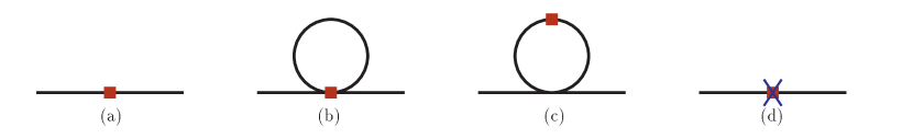
Figure 1: One-loop diagrams contributing to the form factors. The square stands for the insertion of the vector external current. The cross indicates an ${\cal O}(p^{4})$ vertex from ${\cal L}_{4}$.

Once quantum corrections are taken into account, loops of pseudoscalars can appear and the Lagrangian ${\cal L}_{4}$ starts to contribute. At next-to-leading order we have the three types of contributions depicted in Fig. 1, as well as wave-function renormalization. The diagrams are: i) the tree level diagrams giving a polynomial in quark masses and external momenta whose coefficients depend on the LECs of (2.2) via the diagram in Fig 1(d). ii) the tadpole diagrams which contribute a logarithmic dependence on the quark masses from Fig. 1(b). In the present case these vanish because of the requirement (3.6) when combined with the contributions from wave-function renormalization. iii) the unitarity correction due to rescattering shown in Fig. 1(c).

We regulate using dimensional regularization and use the modified $\overline{\mbox{MS}}$ subtraction scheme as is standard in ChPT [4, 5].

Our results are in agreement with those presented in [12, 13] and can be written in the form

$$\left.F^{\pi}_{V}(t)\right|_{p^{4}} = \frac{1}{F_{\pi}^{2}}\left(2\,{\cal H}(m_{\pi}^{2},m_{\pi}^{2},t)+{\cal H}(m_{K}^{2},m_{K}^{2},t)\right)\,,$$

$$\left.F^{K^{+}}_{V}(t)\right|_{p^{4}} = \frac{1}{F_{\pi}^{2}}\left({\cal H}(m_{\pi}^{2},m_{\pi}^{2},t)+2\,{\cal H}(m_{K}^{2},m_{K}^{2},t)\right)\,,$$

$$\left.F^{K^{0}}_{V}(t)\right|_{p^{4}} = \frac{1}{F_{\pi}^{2}}\left(-{\cal H}(m_{\pi}^{2},m_{\pi}^{2},t)+{\cal H}(m_{K}^{2},m_{K}^{2},t)\right)\,.$$ (3.8)

In terms of the integrals defined in App. B, the function ${\cal H}$ is defined by

$${\cal H}(m^{2},m^{2},t)=\frac{1}{2}\bar{A}(m^{2})-\bar{B}_{22}(m^{2},m^{2},t)+\frac{2}{3}\,tL_{9}^{r}\,.$$ (3.9)

The form factors to ${\cal O}(p^{4})$ obviously satisfy the relation

$$\left.F^{\pi}_{V}(t)\right|_{p^{2}+p^{4}}=\left.F^{K^{+}}_{V}(t)\right|_{p^{2}+p^{4}}-\left.F^{K^{0}}_{V}(t)\right|_{p^{2}+p^{4}}\,.$$ (3.10)

At this order in the chiral expansion the expressions for the form factors depend on a single LEC, namely $L_{9}^{r}$, providing an opportunity for stringent experimental tests. This was discussed in detail in [12] with the then available data and will be discussed in Sect. 5.

The choice of the pion decay constant $F_{\pi}$ in (3.2) is a matter of choice. We could equally well have chosen $F_{0}$, the decay constant in the chiral limit, or $F_{K}$. The difference is ${\cal O}(p^{6})$.

3.3 Next-to-next-to-leading form factors

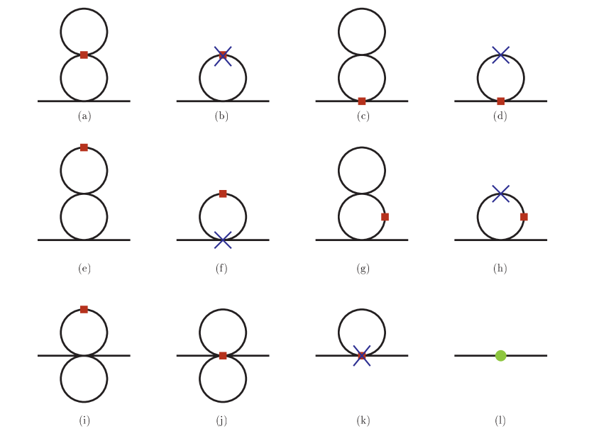
Figure 2: The factorizable two-loop diagrams, one-loop diagrams with vertices from ${\cal L}_{4}$, and the tree level diagram with an ${\cal L}_{6}$ vertex, contributing to the form factors. The square stands for the insertion of the vector external current. A cross indicates a vertex from ${\cal L}_{4}$ and a filled circle a vertex from ${\cal L}_{6}$.

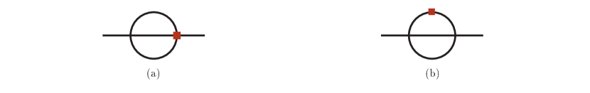
Figure 3: Non-factorizable two-loop diagrams contributing to the form factors. The square stands for the insertion of the vector external current. There exists also a crossed version of diagram (a), with the vector current insertion on the left hand side.

3.3.1 General techniques and checks

In order to obtain the expression for the form factors to ${\cal O}(p^{6})$ accuracy, one has to consider the diagrams of Figs. 2 and 3 in addition to wave-function renormalization contributions to the same order. At two-loops a whole set of new complications surface as compared to one-loop and especially the regularization and renormalization procedure has to be dealt more carefully. A long description tailored to ChPT can be found in Ref. [19], and issues relevant to definitions of the subtraction are also treated in [20].

There are many ways in which to organize the calculation. One alternative is to use the one-loop expressions as generalized vertices and propagators in the two-loop calculation. This shortens the algebra but requires the knowledge of many one-loop processes also for off-shell external particles. We chose instead to perform explicitly the calculation of all Feynman diagrams in terms of lowest order quantities and afterwards put these into the physical quantities. A number of cancellations have to occur for both methods to agree and these, described below, form one of the checks on our calculation.

Our calculations are made in dimensional regularization with the choice $d=4-2\epsilon$. In order to include all finite contributions in $d=4$, it is needed to keep loop integrals and constants in the diagrams of Fig. 2 to order $\epsilon$. In general any function, $f(m^{2}_{i0},q^{2})$, appearing in the loop diagrams has a Laurent expansion in $\epsilon$;

$$f(m_{i0}^{2},q^{2})=\frac{1}{\epsilon^{2}}f^{(-2)}(m_{i0}^{2},q^{2})+\frac{1}{\epsilon}f^{(-1)}(m_{i0}^{2},q^{2})+f^{(0)}(m_{i0}^{2},q^{2})+\epsilon f^{(1)}(m_{i0}^{2},q^{2})+{\cal O}(\epsilon^{2})\,.$$ (3.11)

We never encounter terms more divergent than $1/\epsilon^{2}$ and terms higher order in the expansion do not contribute to the order we work. The superscripts indicate the power of $\epsilon$ the coefficient function gets multiplied with. As an example, diagram (d) in Fig. 2 contains two key ingredients: the one-loop two point function $B$ (see Appendix B) and the constants, $L$, appearing in ${\cal L}_{4}$, Eq. (2.2). Expanding both of them in Laurent series, one gets the following naive finite contributions

$$\mbox{diagram (d)}|_{\mbox{\tiny finite}}\rightarrow a_{1}B^{(-1)}L^{(1)}+a_{2}B^{(0)}L^{(0)}+a_{3}B^{(1)}L^{(-1)}\,,$$ (3.12)

with $a_{i}$ some polynomial that depends on the masses and/or external momenta. As shown in [20], the constants $L^{(1)}$ can be chosen to be zero, their effect can be absorbed in the values of the ${\cal O}(p^{6})$ constants $C_{i}$. We will do so. The contribution containing $B^{(1)}$ can be shown to always have counterparts cancelling it in other diagrams. This however requires a careful evaluation of all diagrams that makes this cancellation apparent and in particular, requires careful treatment of parts of the nonfactorizable diagrams. We have evaluated the latter in a more general fashion and we are thus obliged to keep the contributions containing $B^{(1)}$.

Regularization and renormalization:

In a local field theory, the final divergences are always polynomial in the masses and momenta. These can thus be subtracted from the freedom in the choice of parameters in the tree level Lagrangian. We use here the standard ChPT $\overline{\mbox{MS}}$ subtraction with e.g. for the coefficients of ${\cal L}_{4}$

$$L_{i}=\left(e^{c}\mu\right)^{d-4}\left(\frac{\gamma_{i}}{16\pi^{2}(d-4)}+L_{i}^{r}(\mu)\right)$$ (3.13)

and

$$c=-\frac{1}{2}\left(\ln(4\pi)+\Gamma^{\prime}(1)+1\right)\,.$$ (3.14)

Notice that Eq. (3.13) implies a choice of $L^{(1)}_{i}$ as mentioned above.

To ${\cal O}(p^{4})$ there are no problems and all divergences occurring diagram by diagram are polynomial. This is no longer true at ${\cal O}(p^{6})$ where there are two sources of nonpolynomial divergences. We have the one-loop diagrams with insertions of ${\cal L}_{4}$ vertices. The nonpolynomial part of the loop integrals is multiplied with (3.13) and leads to divergences proportional to $\ln(M^{2}/\mu^{2})$ and others with momentum dependence. The required cancellation of these divergences leads to so called Weinberg relations. From the one-loop diagrams with ${\cal L}_{4}$ vertices we can determine the nonpolynomial divergences of the two-loop diagrams. These in turn determine the double poles.

As an example of the above, the $t$ dependent part of the nonlocal divergence produced by the diagram of Fig. 2(f) must be cancelled by other diagrams having the same possible divergence, in this case the diagrams of Fig. 2(a,b,e,g,h,i) and of Fig. 3(b). The cancellation of both the $t$ dependent and the $\ln(M^{2}/\mu^{2})$ dependent divergences is a very strong check on our calculation.

Double logarithms: The cancellation as discussed above, can in fact be used to calculate part of the ${\cal O}(p^{6})$ correction using only one-loop diagrams. This has been done for quite a few processes in Ref. [21]. In the two-flavour case for many quantities these so called double-logarithm contributions often dominate, in particular they do so for $\pi\pi$-scattering and the corrections to the masses, [22, 15] but not for e.g. the pion form factor [15]. Our results here agree with the double-logarithm part as calculated in [21].

Terms of the type $L_{i}^{r}(\mu)\times L_{j}^{r}(\mu)$: Similarly to the previous contribution the $L_{i}^{r}(\mu)\times L_{j}^{r}(\mu)$ pieces can be obtained in full generality without a complete calculation, since they only occur via tree diagrams and were also calculated in [21]. Our results agree with those given there.

Irreducible two-loop integrals: One of the main features of the non-factorizable integrals at two-loop (see Fig. (3)) in the three flavour case is that they can contain different scales even at zero momentum transfer. Those scales are given by the pseudoscalar masses. No exact analytic expressions are known for all the integrals we need here. Given the complexity of the integrals, it is worthwhile to have as many cross-checks on the numerical evaluation as possible. We differentiate between the two topologies in Fig. (3). The topology (a) is calculated with the methods described in [7]. In particular, the subtraction constants are derived using the methods of [23, 24], of which we obtained an alternative derivation of the recursion relations, and the dispersive part with a generalization of the methods of [25] to different masses. In addition we cross-checked the results using the techniques in [26, 27].

For the topology (b) we used the methods given in [26, 27] and cross-checked with [25] for the case of equal masses. As an independent check for the tensor structures, we evaluate most of them numerically and then check that they satisfy the relations derived using the methods of Passarino and Veltman [28], between the various different Lorentz structures.

Putting the result in physical quantities: Up to this level we have computed all the diagrams in terms of the quantities appearing in the Lagrangian. In particular we have used the decay constant in the chiral limit and the lowest order meson masses. Once the amplitude is finite in terms of these bare quantities, with a cancellation of all nonlocal and nonpolynomial divergences as well as agreement of the polynomial divergences with the general evaluation of [20], we must rewrite these bare masses and decay constants in terms of the physical ones. As was mentioned already, the leading order in the form factors are mere constants fixed by Ward identities, Eq. (3.6). We thus only need the ${\cal O}(p^{4})$ expressions for masses and decay constants to do this rewriting. This is one of the reasons that the expressions here are so much simpler than in the $K_{\ell 4}$ case performed earlier, allowing us to quote the full result for the pion form factor, not only a numerical parametrization.

There is of course a certain choice in how this writing in physical decay constants is done. At lowest order $F_{\pi}\equiv F_{K}\equiv F_{\eta}=F_{0}$ but at higher orders nothing prevents us to write the ${\cal O}(p^{4})$ expressions with $F_{K}$ or $F_{\eta}$, rather than $F_{\pi}$.

For the masses the situation is easier in this case as well, the $\eta$ does not appear in the ${\cal O}(p^{4})$ result, so the full ${\cal O}(p^{4})$ result can be simply written in terms of the pion and kaon mass. The masses can appear inside the arguments of the loop integrals. Rewriting those in the physical masses we expand the function in a Taylor series around the value of the mass at the next-to-leading order

$$f(m_{i0}^{2};q^{2})=f(m_{i}^{2};q^{2})+\sum_{j}\left(m_{j0}^{2}-m_{j}^{2}\right)\frac{\partial}{\partial m_{j0}^{2}}f(m_{i0}^{2};q^{2})|_{m_{i0}=m_{i}}\,.$$ (3.15)

For instance, for the scalar one and two-point functions, $A$ and $B$, one obtains

$$A(m_{\pi 0}^{2}) = A(m_{\pi}^{2})+\left(m_{\pi 0}^{2}-m_{\pi}^{2}\right)B(m_{\pi}^{2},m_{\pi}^{2};0)\,,$$

$$B\left(m_{\pi 0}^{2},m_{K0}^{2};q^{2}\right) = B(m_{\pi}^{2},m_{K}^{2};q^{2})+\left(m_{\pi 0}^{2}-m_{\pi}^{2}\right)C(m_{\pi}^{2},m_{\pi}^{2},m_{K}^{2};q^{2})$$ (3.16)

$$+\left(m_{K0}^{2}-m_{K}^{2}\right)C(m_{K}^{2},m_{K}^{2},m_{\pi}^{2};q^{2})\,,$$

where the $m_{i0}^{2}$ are the bare or lowest order quantities and the $m_{i}^{2}$ are the equivalent renormalized masses at next-to-leading order. Finally the $C$ function is the scalar three point function

$$C(m_{1}^{2},m_{2}^{2},m_{3}^{2},q^{2})=\frac{1}{i}\int\,d^{d}p\frac{1}{\left(p^{2}-m_{1}^{2}\right)\left(p^{2}-m_{2}^{2}\right)\left((p-q)^{2}-m_{3}^{2}\right)}\,.$$ (3.17)

Once these steps are performed, we are allowed to identify the masses and decay constants with the physical ones. Notice that this identification can be done without any manipulation in the genuine two-loop topologies from the very beginning because the difference is of higher order. As a consistency check, we have cross-checked that all our final expressions are scale invariant. Notice that both the lowest order masses and decay constants and the physical ones are finite and this rewriting does not introduce any infinities.

Three-point one-loop integrals: There is an extra check on the way that we performed the renormalization of the masses and decay constants. As is evident the diagrams (a,b,c,d,g) and (h) in Fig. (2) can be obtained by substituting the “bare propagator” of diagrams (b,c) in Fig. (1) by a “dressed” one-loop one. In this last method only one and two-propagator loop functions are permitted. In particular this tells us that the three-point functions, $C$, appearing naively via diagrams (g) and (h) should disappear once we promote all bare quantities to the physical ones.

Gell-Mann–Okubo relation: There is one last comment concerning higher order corrections. At ${\cal O}(p^{6})$ we have chosen to rewrite all masses, except those inside logarithms and loop functions, in terms of the pion and kaon mass. The quark masses are written into those and the $\eta$ mass is removed using the GMO relation in the SU(2) isospin limit,

$$3m_{\eta}^{2}=4m_{K}^{2}-m_{\pi}^{2}\,.$$ (3.18)

As mentioned above already, the vector form factors do not depend on the eta mass at next-to-leading order, only at next-to-next-to-leading order. This is not necessarily the case for other quantities, in particular the scalar form factors. Numerically at low transfer momentum the difference in using or not Eq. (3.18) for the $\eta$ mass in the remaining loop functions is small.

Independence of $\mu$: A final check on the numerical programs is that they are independent of the scale $\mu$ when this scale is varied in the evaluation of the integrals and the values of the constants are changed appropriately.

Comparison with previous work: As an independent cross-check of our calculations we compared whenever possible with the available expressions in the literature. This is the case for the $K^{0}$ form factor which was obtained up to next-to-next-to-leading order in [17] for the isospin limiting case. We have compared partially our results for the same process and find agreement with the double logarithm terms and with the pieces containing the irreducible integrals. The same authors considered previously, [16], a certain combination for the vector form factor that leads to the Sirlin’s relation [29]. The $q^{2}$ dependence of this relation is free of unknown constants of ${\cal O}(p^{6})$ because of the Ademollo-Gatto theorem [30]. Some expressions for the pion form factor are also in the recent paper [18]. The analytical comparison with this expression can only be made between the pieces obtained via the reducible diagrams finding agreement between them. For the rest of the expression, irreducible diagrams, the authors of [16, 18] use like us a numerical approach. The results of these are in good agreement.

FORM: Most of the algebraic manipulations needed for this work were performed using FORM 1.0 and FORM 3.0 [31] while independent cross-checks of some structures were performed by hand.

3.3.2 Results

We split the full ${\cal O}(p^{6})$ contribution in several pieces

$$\left.F_{V}^{P}(t)\right|_{p^{6}}=\frac{1}{F_{\pi}^{4}}\left(F_{V\mathbf{L}}^{P}(t)+F_{V\mathbf{C}}^{P}(t)+F_{V\mathbf{B}}^{P}(t)+F_{V\mathbf{H}}^{P}(t)+F_{V\mathbf{V}}^{P}(t)\right)\,,$$ (3.19)

with the following definitions:
$F_{V\mathbf{L}}^{P}(t)$: The part which depends on the $L_{i}^{r}$. $F_{V\mathbf{C}}^{P}(t)$: The polynomial dependence on the ${\cal L}_{6}$ parameters $C_{i}^{r}$. $F_{V\mathbf{B}}^{P}(t)$: The part with the loop integrals that can be done analytically. $F_{V\mathbf{H}}^{P}(t)$: The part that depends on the sunset integrals. $F_{V\mathbf{V}}^{P}(t)$: The part containing the irreducible two-loop vertex integrals.
The last three contain the proper two-loop diagrams and are the hardest part of the calculation. The precise separation between them is somewhat dependent on how the set of nonfactorizable two-loop integrals is chosen. In addition, there are rather large numerical cancellations between these three parts because the method to separate factorizable from nonfactorizable contributions often induces large terms in both which afterwards cancel.

We have not performed the separation into tadpole and unitarity corrections here. Because of the requirement (3.6) the tadpoles cancel to a very large extent and the separation between tadpole and unitarity contributions is in any case representation dependent.

The dependence on the $L_{i}^{r}$ is fairly simple:

$$F_{V\mathbf{L}}^{\pi}(q^{2}) = 8m_{\pi}^{2}\left(2L_{4}^{r}+L_{5}^{r}\right)\bar{A}(m_{\pi}^{2})+4m_{\pi}^{2}L_{5}^{r}\bar{A}(m_{K}^{2})+q^{2}L_{9}^{r}(6\bar{A}(m_{\pi}^{2})+3\bar{A}(m_{K}^{2}))$$ (3.20)

$$+\bar{B}_{22}(m_{\pi}^{2},m_{\pi}^{2};q^{2})\left\{-16m_{\pi}^{2}(2L_{4}^{r}+L_{5}^{r})+4q^{2}(4L_{1}^{r}-2L_{2}^{r}+2L_{3}^{r}-L_{9}^{r})\right\}$$

$$+\bar{B}_{22}(m_{K}^{2},m_{K}^{2};q^{2})\left\{-8m_{\pi}^{2}L_{5}^{r}+4q^{2}L_{3}^{r}-2q^{2}L_{9}^{r}\right\}\,,$$

$$F_{V\mathbf{L}}^{K^{+}}(q^{2}) = \left(16m_{K}^{2}L_{4}^{r}+8m_{\pi}^{2}L_{5}^{r}\right)\bar{A}(m_{K}^{2})+4m_{\pi}^{2}L_{5}^{r}\bar{A}(m_{\pi}^{2})+q^{2}L_{9}^{r}(5\bar{A}(m_{\pi}^{2})+4\bar{A}(m_{K}^{2}))$$ (3.21)

$$+\bar{B}_{22}(m_{K}^{2},m_{K}^{2};q^{2})\left\{-32m_{K}^{2}L_{4}^{r}-16m_{\pi}^{2}L_{5}^{r}+4q^{2}(4L_{1}^{r}-2L_{2}^{r}+2L_{3}^{r}-L_{9}^{r})\right\}$$

$$+\bar{B}_{22}(m_{\pi}^{2},m_{\pi}^{2};q^{2})\left\{-8m_{\pi}^{2}L_{5}^{r}+4q^{2}L_{3}^{r}-2q^{2}L_{9}^{r}\right\}$$

$$16L_{5}^{r}L_{9}^{r}q^{2}\left(m_{\pi}^{2}-m_{K}^{2}\right)\,,$$

and

$$F_{V\mathbf{L}}^{K^{0}}(q^{2}) = \left(4m_{\pi}^{2}L_{5}^{r}+q^{2}L_{9}^{r}\right)\,\left(-\bar{A}(m_{\pi}^{2})+\bar{A}(m_{K}^{2})\right)$$ (3.22)

$$+\bar{B}_{22}(m_{\pi}^{2},m_{\pi}^{2};q^{2})\left\{8m_{\pi}^{2}L_{5}^{r}-2q^{2}(2L_{3}^{r}-L_{9}^{r})\right\}$$

$$+\bar{B}_{22}(m_{K}^{2},m_{K}^{2};q^{2})\left\{-8m_{\pi}^{2}L_{5}^{r}+2q^{2}(2L_{3}^{r}-L_{9}^{r})\right\}\,.$$

We can now check how large the various loop contributions are. In Fig. 4 we have shown the real and imaginary parts of the pure loop contributions at ${\cal O}(p^{4})$ and ${\cal O}(p^{6})$ for the pion form factor.

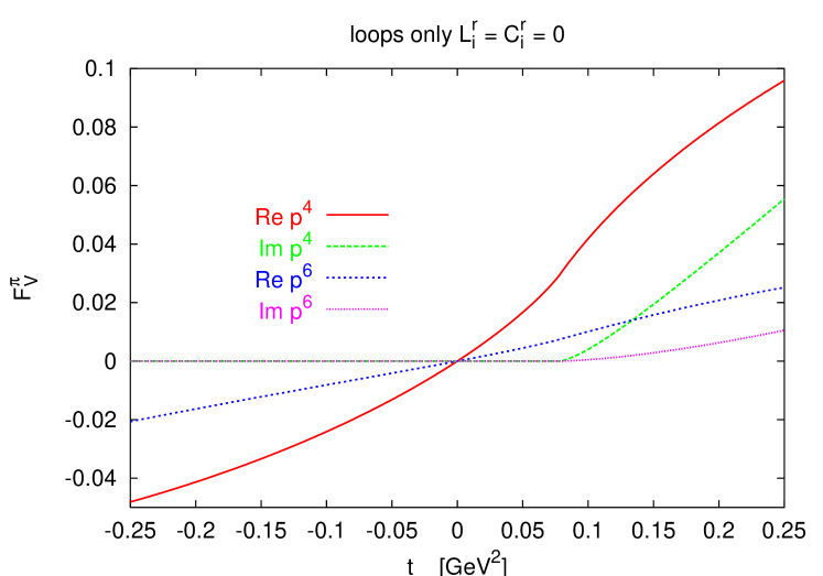
Figure 4: The real and imaginary parts of the loop diagrams at ${\cal O}(p^{4})$ and ${\cal O}(p^{6})$ with all $L_{i}^{r}=0$, for the pion form factor. Notice that there is convergence both for the real and the imaginary part.

To put the figures in perspective one should bear in mind that the lowest order is exactly one and that at $t=\pm 0.25$ GeV² the ${\cal O}(p^{4})$ contribution from $L_{9}^{r}$ setting $L_{9}^{r}=6.9\times 10^{-3}$ is $\pm 0.40$. We show the difference between the contribution from the pure loops only for the three different pseudoscalars in Fig. 5 at ${\cal O}(p^{4})$ and in Fig. 6 at ${\cal O}(p^{6})$.

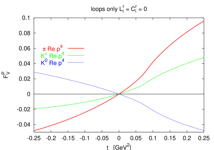
Figure 5: The real parts of the loop diagrams at ${\cal O}(p^{4})$ for the pion, charged kaon and neutral kaon form factor.

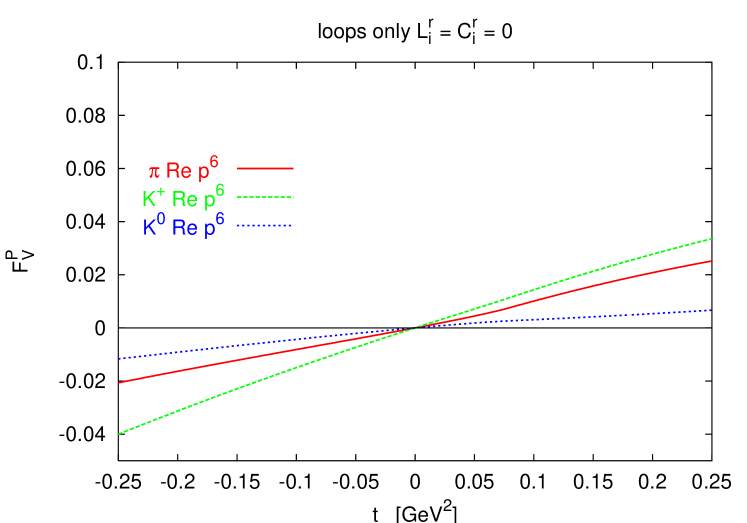
Figure 6: The real parts of the loop diagrams at ${\cal O}(p^{6})$ with all $L_{i}^{r}=0$, for the pion, charged kaon and neutral kaon form factor. The scale is the same as in Fig. 5.

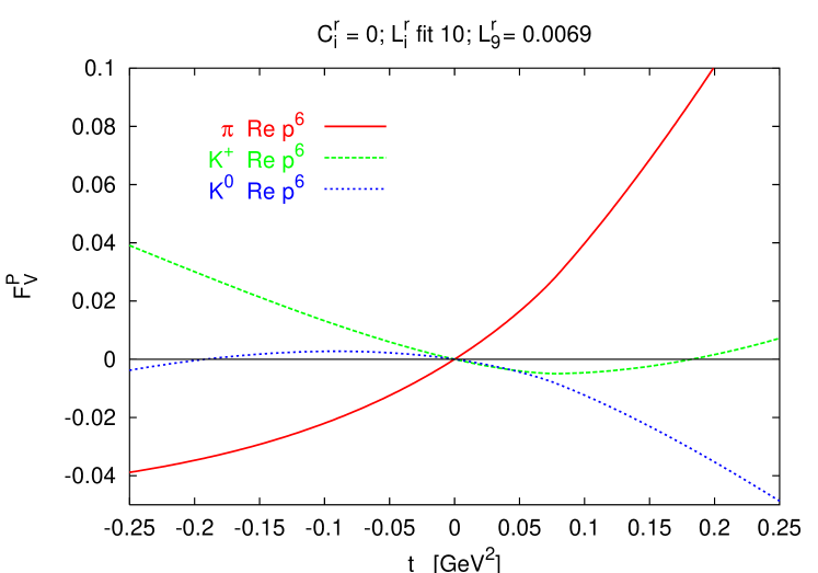
Figure 7: The real parts at ${\cal O}(p^{6})$ for the pion, charged kaon and neutral kaon form factor that depend on $L_{i}^{r}$. This corresponds to $F_{V\mathbf{L}}^{P}(t)$. The inputs are taken from [10]. The scale is the same as in Fig. 5.

Fig. 7 shows the contribution from the $L_{i}^{r}$ dependent part at ${\cal O}(p^{6})$, $F_{V\mathbf{L}}^{P}(t)$ with the input parameters as given in [10].

The part that depends on the ${\cal L}_{6}$ constants $C_{i}^{r}$ is also rather short.

$$F_{V\mathbf{C}}^{\pi}(q^{2}) = -4q^{2}m_{\pi}^{2}(4C^{r}_{12}+4C^{r}_{13}+2C^{r}_{63}+C^{r}_{64}+C^{r}_{65}+2C^{r}_{90})$$ (3.23)

$$-8q^{2}m_{K}^{2}(4C^{r}_{13}+C^{r}_{64})-4q^{4}(C^{r}_{88}-C^{r}_{90})\,,$$

$$F_{V\mathbf{C}}^{K^{+}}(q^{2}) = -q^{2}m_{\pi}^{2}\left(16C^{r}_{13}+\frac{8}{3}C^{r}_{63}+4C^{r}_{64}-\frac{4}{3}C^{r}_{65}\right)$$ (3.24)

$$-q^{2}m_{K}^{2}\left(16C^{r}_{12}+32C^{r}_{13}+\frac{16}{3}C^{r}_{63}+8C^{r}_{64}+\frac{16}{3}C^{r}_{65}+8C^{r}_{90}\right)$$

$$-4q^{4}\left(C^{r}_{88}-C^{r}_{90}\right)\,,$$

and

$$F_{V\mathbf{C}}^{K^{0}}(q^{2}) = \frac{8}{3}q^{2}(m_{\pi}^{2}-m_{K}^{2})(2C^{r}_{63}-C^{r}_{65})\,.$$ (3.25)

At low-energies, for instance the space-like interval with $\sqrt{-t}\lesssim 350$ MeV, the pion vector form factor can be expanded in a Taylor series as

$$F_{V}^{\pi}(t)=1+\frac{1}{6}\langle r^{2}\rangle_{V}^{\pi}t+c_{V}^{\pi}t^{2}+{\cal O}(t^{3})\,,$$ (3.26)

defining in that manner the radii,$\langle r^{2}\rangle_{V}^{P}$, and the coefficient $c_{V}^{P}$.

3.4 Isospin breaking

Throughout this paper we work in the isospin limit. The isospin breaking contributions can be split naively into two parts.

A first contribution comes through electromagnetic interactions. This has been studied for the pion form factor in [32]. This is primarily obtained by taking photon loops that develop an infra-red singularity. Near threshold in the time-like region this contribution can dominate over the next-to-next-to-leading terms because of Coulomb final state interactions. This is not the case for the pion form factor itself, the corrections are about $1\%$. For the constant $c_{V}^{\pi}$ there might be a large contribution coming from resolution dependent terms but they cancel to a large extent for typical values of the detector resolution. The electromagnetic contribution to the masses we take into account indirectly, we use the charged pion and charged kaon mass in our numerical analysis.

The second source of isospin breaking is from the mass difference $m_{u}-m_{d}$. The pion form factor receives corrections starting only at ${\cal O}\left((m_{d}-m_{u})^{2}\right)$ [30]. This together with the constraint (3.6) means that corrections only come from loop diagrams and are thus expected to be small. In the kaon form factors isospin breaking could be larger but given the present experimental accuracy is not expected to be relevant.

4 Data and fits with the ChPT expression

4.1 Data on $F_{V}^{\pi}$

Data on the pion form factor have been collected in both time-like, $t>0$, and space-like, $t<0$, regions. We discuss both in turn.

4.1.1 Space-like

In the space-like region the measurements have been done using $\pi e\to\pi e$ scattering. There are two main experiments [33] at FNAL and NA7 at CERN [34]. Both experiments are based on pions scattering off the electrons of a liquid hydrogen target and the data agree in the overlap region. The last one has significantly smaller error bars and dominates clearly all the fits. There are also somewhat older FNAL data from the same experiment using a lower energy pion beam [35]. These have larger errors and are compatible with the newer data. References to older data can be found in both [34] and [33]. These data were analyzed in both papers with a pole-fit

$$F_{V}^{\pi}(t)=\frac{n}{\left(1-\frac{1}{6}\langle r^{2}\rangle_{V}^{\pi}t\right)^{2}}\,,$$ (4.1)

where n refers to the normalization uncertainty. Ref. [34] obtained

$$\langle r^{2}\rangle_{V}^{\pi}=(0.431\pm 0.010)~{}\mbox{fm}^{2}$$ (4.2)

when they constrained $n$ and

$$\langle r^{2}\rangle_{V}^{\pi}=(0.427\pm 0.010)~{}\mbox{fm}^{2}$$ (4.3)

with $n$ left free. The equivalent results of [33] are

$$\langle r^{2}\rangle_{V}^{\pi}=(0.439\pm 0.030)~{}\mbox{fm}^{2}$$ (4.4)

when they constrained $n$ and

$$\langle r^{2}\rangle_{V}^{\pi}=(0.384\pm 0.088)~{}\mbox{fm}^{2}$$ (4.5)

with $n$ left free.

Data	$n$	$\langle r^{2}\rangle_{V}^{\pi}$ [fm2]
FNAL [33]	$0.973\pm 0.033$	$0.382\pm 0.078$
	$\equiv 1$	$0.443\pm 0.018$
NA7 [34]	$0.990\pm 0.004$	$0.428\pm 0.011$
	$\equiv 1$	$0.452\pm 0.006$

Table 1: The parameters of a simple pole fit to the $\pi e$ scattering data. Note the difference with the normalization free.

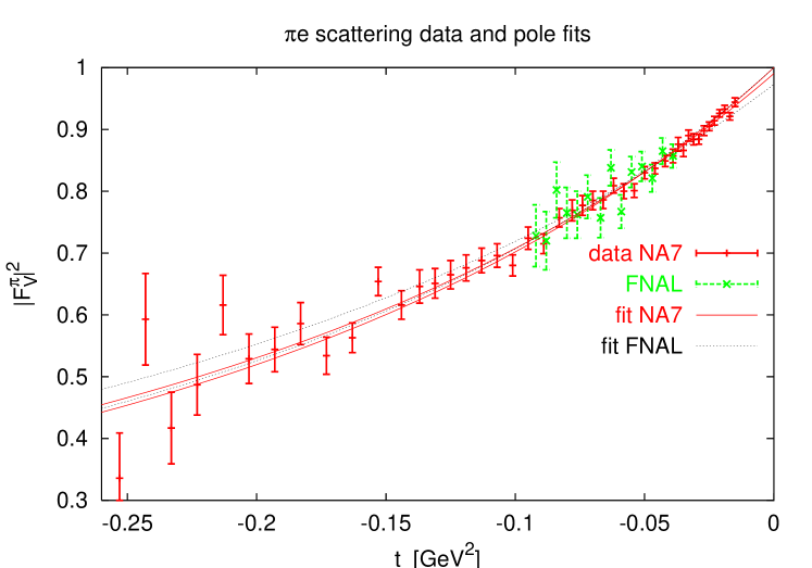
Figure 8: The two data sets of $\pi e$ scattering and the resulting pion form factor squared. Also shown are pole fits to both data sets.

The two data sets together with the results of our own pole fits are shown in Fig. 8 and the pole fit parameters are in Table 1. The difference with the numbers quoted by the experiments themselves is because there the normalization was fixed using the experimental error rather than set exactly equal to one. The quoted errors for the normalization are 1% for [33] and 0.9% for [34].

Using the previous data sets there are several determinations of the pion vector form factor in the literature. The experiments were analyzed directly mainly with a pole fit as discussed above. A full analysis within the framework of two flavour ChPT is in Ref. [15], and we will compare with the results from there in Sect. 5.

In [34] the data were also analyzed using a dispersion relation technique with a Padé approximation for the Omnés representation and $\pi\pi$ data for the $\delta_{1}^{1}$ phase shift the result they obtained is

$$\langle r^{2}\rangle_{V}^{\pi}=(0.439\pm 0.008)\,\mbox{fm}^{2}\,.$$ (4.6)

Details of this technique can be found in [36].

4.1.2 Time-like

In the time-like region there are several experiments, but unfortunately most of the data is located outside the range of applicability of ChPT. Essentially the data is obtained from two sources: $\tau\rightarrow\pi\pi\nu_{\tau}$ [37] and $e^{-}e^{+}\rightarrow\pi^{+}\pi^{-}$ [38, 39, 40, 41]. In the later experiment, [41], corresponding to the NA7 collaboration, the systematic errors are close to the statistical ones and we believe that they have been underestimated in the time-like region as they are difficult to fit together with the space-like data.

A resonance based model was used in [39] to fit the data up to 1.2 GeV and determines the mass and decay constants of the $\rho$ as well as the pion radius with the result

$$\langle r^{2}\rangle_{V}^{\pi}=(0.460\pm 0.011)\,\mbox{fm}^{2}\,.$$ (4.7)

Instead one can rely on $\tau\rightarrow\pi\pi\nu_{\tau}$ data to fit the expression

$$F_{V}^{\pi}(t)=exp\left\{\alpha_{1}t+\frac{1}{2}\alpha_{2}t^{2}+\frac{t^{3}}{\pi}\int_{4m_{\pi}^{2}}^{\infty}\frac{dz}{z^{3}}\frac{\delta_{1}^{1}}{z-t-i\epsilon}\right\}\,,$$ (4.8)

with $\alpha_{1},\alpha_{2}$ given in terms of $\langle r^{2}\rangle_{V}^{\pi}$ and $c_{V}^{\pi}$ (see [42]) and $\delta_{1}^{1}$ determined by resonance saturation. Keeping only the $\rho$ contribution one obtains

$$\langle r^{2}\rangle_{V}^{\pi}=(0.429\pm 0.01)\,\mbox{fm}^{2}\,.$$ (4.9)

4.2 Data on $F_{V}^{K^{+}}$

The charged kaon form factor has been measured directly via kaon electron scattering method by the same two main experiments that measured the pion form factor. The older experiment is a FNAL experiment [43] and reported a rather low kaon charge radius obtained by a fit to a pole form factor

$$\langle r^{2}\rangle_{V}^{K^{+}}=(0.28\pm 0.05)~{}\mbox{fm}^{2}\,.$$ (4.10)

They also quoted a dipole fit where the normalization was left free with the result

$$\langle r^{2}\rangle_{V}^{K^{+}}=(0.42\pm 0.20)~{}\mbox{fm}^{2}\,.$$ (4.11)

In [33] a simultaneous analysis of the pion and kaon form factors was performed from the obtained data quoting the difference

$$\langle r^{2}\rangle_{V}^{K^{+}}-\langle r^{2}\rangle_{V}^{\pi}=(-0.16\pm 0.06)~{}\mbox{fm}^{2}\,.$$ (4.12)

This difference is claimed to be largely free of systematic errors.

The more recent CERN experiment [44] finds using pole-like fits

$$\langle r^{2}\rangle_{V}^{K^{+}}=(0.34\pm 0.05)~{}\mbox{fm}^{2}\,,$$ (4.13)

and from the ratio to the simultaneously collected pion data

$$\langle r^{2}\rangle_{V}^{K^{+}}-\langle r^{2}\rangle_{V}^{\pi}=(-0.10\pm 0.045)~{}\mbox{fm}^{2}\,.$$ (4.14)

Both data sets are shown in Fig. 9 together with a simple pole fit with the normalization fixed to 1 and left free to both data sets.

Figure 9: The two data sets of $Ke$ scattering and the resulting kaon form factor squared. Also shown are pole fits to both data sets.

The parameters of those fits are in Table 2.

Data	$n$	$\langle r^{2}\rangle_{V}^{K^{+}}$ [fm2]
FNAL [43]	$1.084\pm 0.091$	$0.457\pm 0.198$
	$\equiv 1$	$0.278\pm 0.046$
NA7 [44]	$1.019\pm 0.030$	$0.395\pm 0.109$
	$\equiv 1$	$0.334\pm 0.045$

Table 2: The parameters of a simple pole fit to the $Ke$ scattering data. Note the difference with the normalization free.

The threshold for kaon production in tau decays or $e^{+}e^{-}$ annihilation is too high for the ChPT expressions to be valid. In principle a dispersion relation could be used to relate those data with the threshold parameters but this involves a rather large extrapolation. We have therefore not included this type of data in our analysis.

4.3 Data on $F_{V}^{K^{0}}$

The data on the neutral kaon electromagnetic form factor are rather scarce. There is a measurement of the radius using kaon regeneration on electrons [45] leading to

$$\langle r^{2}\rangle_{V}^{K^{0}}=(-0.054\pm 0.026)~{}\mbox{fm}^{2}\,.$$ (4.15)

The decay $K_{L}\to\pi^{+}\pi^{-}e^{+}e^{-}$ also has contributions that contain the neutral kaon electromagnetic form factor but the extraction from the data is rather model dependent and not yet done at present.

4.4 Input parameters

For the physical masses we use the charged pion and kaon mass [46] and the pion decay constant,

$$m_{\pi^{+}}=139.56995~{}\mbox{MeV}\,,\quad m_{K^{+}}=493.677~{}\mbox{MeV}\,\mbox{ and }F_{\pi}=92.4~{}\mbox{MeV}\,.$$ (4.16)

For the eta mass we use the mass resulting from the GMO relation. As discussed above, this does not make any difference within the accuracy of our results.

A somewhat more complicated issue is how to deal with the input values of the $L_{i}^{r}$ other than $L_{9}^{r}$. We use the two-loop accuracy determination given in fit 10 of [10]. We choose fit 10 and not the main fit, because the analysis of the E865 experiment has been confirmed in the meantime [47]. Notice that in doing so, i.e. using the values in [10] without any new refitting, we have assumed that the value of $L_{9}^{r}$ does not have a substantial impact on the rest of LECs. This is true, as we discussed in [8]. For the quantities studied in [10] $L_{9}^{r}$ only appears inside the $K_{\ell 4}$ form factors, but together with the squared effective mass of the dilepton system and varying $L_{9}^{r}$ over an extremely wide range did not change the fitting results.

4.5 ChPT fits to $F_{V}^{\pi}(t)$

Checking the $L_{9}^{r}$ dependence of $F_{V}^{\pi}$, we find that the real part of this can be well described by a polynomial of the form

$$\left.F_{V}^{\pi}(t)\right|_{p^{6},\,L_{9}^{r}}=L_{9}^{r}\,\left(at+bt^{2}+ct^{3}\right)\,.$$ (4.17)

The coefficients $a$, $b$ and $c$ are in principle dependent on the other $L_{i}^{r}$ used as input.

We fit the data on $F_{V}^{\pi}(t)$ with the ChPT expressions with the value of $L_{9}^{r}$ set equal to zero and a polynomial of the form

$$a_{f}t+b_{f}t^{2}+c_{f}t^{3}$$ (4.18)

for several variations of the input. In this way we can separate the dependence of $L_{9}^{r}$ on the unknown ${\cal O}(p^{6})$ constants. We fit similarly at ${\cal O}(p^{4})$.

In the fit we have left the normalization of the data from [34], [33] and [41] as an additional fit parameter.

	$n$[34]	$n$[33]	$n$[41]	$a_{f}$ [GeV]-2	$b_{f}$ [GeV]-4	$c_{f}$ [GeV]-6
${\cal O}(p^{4})$	0.981	0.979	1.073	$1.285\pm 0.003$	$\equiv 0$	$\equiv 0$
${\cal O}(p^{4})$	0.995	0.998	0.862	$1.647\pm 0.054$	$3.83\pm 0.28$	$5.98\pm 1.69$
${\cal O}(p^{6})$	1.001	1.009	0.871	$1.788\pm 0.045$	$3.16\pm 0.27$	$\equiv 0$
${\cal O}(p^{6})$	0.994	0.998	0.860	$1.693\pm 0.054$	$3.45\pm 0.28$	$5.33\pm 1.69$
${\cal O}(p^{6})$ fit 11	0.994	0.998	0.860	$1.696\pm 0.054$	$3.44\pm 0.28$	$5.32\pm 1.69$
${\cal O}(p^{6})$ fit 12	0.994	0.998	0.860	$1.704\pm 0.055$	$3.43\pm 0.28$	$5.30\pm 1.72$
${\cal O}(p^{6})$ fit 13	0.994	0.998	0.860	$1.690\pm 0.054$	$3.45\pm 0.28$	$5.34\pm 1.69$
polynomial only	0.995	0.998	0.871	$1.936\pm 0.056$	$4.34\pm 0.28$	$6.44\pm 1.69$
${\cal O}(p^{6})$ space	1.000	1.005	–	$1.844\pm 0.018$	$5.53\pm 0.16$	$12.3\pm 1.0$

Table 3: The results of fitting to $F_{V}^{\pi}(t)$ with different theoretical inputs as explained in the text. $\equiv\mbox{a}$ stands for a value held fixed equal to a.

The fits we have performed are a pure ${\cal O}(p^{4})$ fit, an ${\cal O}(p^{4})$ fit but allowing also a $t^{2}$ and $t^{3}$ polynomial, and the same for the ${\cal O}(p^{6})$ expressions. For the input of the $L_{i}^{r}$ we used fit 10 of [10]. The fits to the other $L_{i}^{r}$ with varying the assumptions on $L_{4}^{r}$ and $L_{6}^{r}$ from that reference make essentially no change as can be seen from the rows labelled fit 11, fit 12 and fit 13. We also presented a pure polynomial fit. The $\chi^{2}$ for all the fits including the $t^{3}$ term is the same and the quality of the fit is good. The $\chi^{2}$ is 60.3 for 75 degrees of freedom. The last line indicates the impact of the time-like data. This fit was performed with the space-like data only and had a $\chi^{2}=48.6$ for 54 degrees of freedom.

Notice that the fits are somewhat different, but compatible within errors, with the ones given in [15]. The reason for this difference is that the fits there were performed with the data of [41] with the normalization fixed to one. We have left that free.

4.6 ChPT fits to $F_{V}^{K^{+}}$

We now perform the same fits to the kaon data. The time-like data are very much outside the domain of validity of ChPT so they are not included. The space-like data are much less precise than the pion ones and have a much smaller range of $t$. There will thus be much less information about the higher powers of $t$. For the pion we could fit using the whole region $-0.25\leq t\leq 0.25$, while here we have only the range $-0.11\leq t\leq-0.02$. More care is needed in performing the fits, for instance, fitting with a $t^{3}$ term and both normalizations free leads to rather nonsensical results as can be seen in the sixth row of Table 4.

	$n$[44]	$n$[43]	$a_{f}$ [GeV]-2	$b_{f}$ [GeV]-4	$c_{f}$ [GeV]-6
${\cal O}(p^{4})$	1.015	1.055	$1.408\pm 0.300$	$\equiv 0$	$\equiv 0$
${\cal O}(p^{6})$	0.993	1.028	$0.897\pm 1.169$	$-5.80\pm 11.60$	$\equiv 0$
${\cal O}(p^{6})$	1.015	1.055	$1.464\pm 0.299$	$\equiv 0$	$\equiv 0$
${\cal O}(p^{6})$	1.027	1.070	$1.756\pm 0.297$	$\equiv 3$	$\equiv 0$
polynomial only	0.890	0.919	$-3.259\pm 3.989$	$-96.9\pm 82.0$	$-559\pm 492$
polynomial only	0.993	1.028	$0.978\pm 1.169$	$-5.51\pm 11.60$	$\equiv 0$
polynomial only	1.014	1.054	$1.515\pm 0.300$	$\equiv 0$	$\equiv 0$

Table 4: The results of fitting to $F_{V}^{K^{+}}(t)$ with different theoretical inputs as explained in the text.

4.7 Results for the charge radii and $c_{V}^{P}$

The NLO ChPT expression for the pion form factor [12, 13] was already analyzed quite some time ago, using the space-like data [13]. The results were

$$\langle r^{2}\rangle_{V}^{\pi}=0.392\,(0.366)\,~{}\mbox{fm}^{2}\,,$$ (4.19)

with a fit with normalization one (free).

The analysis using two flavour ChPT at two-loops led to the conclusions [15]

$$\langle r^{2}\rangle_{V}^{\pi}=(0.437\pm 0.016)~{}\mbox{fm}^{2}\,,\quad c_{V}^{\pi}=(3.85\pm 0.60)~{}\mbox{GeV}^{2}$$ (4.20)

including the data of [41] and

$$\langle r^{2}\rangle_{V}^{\pi}=(0.453\pm 0.016)~{}\mbox{fm}^{2}\,,\quad c_{V}^{\pi}=(4.45\pm 0.60)~{}\mbox{GeV}^{2}$$ (4.21)

without including them.

The polynomial fit to all data gives

$$\langle r^{2}\rangle_{V}^{\pi}=(0.452\pm 0.013)~{}\mbox{fm}^{2}\,,\quad c_{V}^{\pi}=(4.34\pm 0.28)~{}\mbox{GeV}^{2}\,.$$ (4.22)

The pure ${\cal O}(p^{4})$ fit yielded

$$\langle r^{2}\rangle_{V}^{\pi}=(0.368\pm 0.001)~{}\mbox{fm}^{2}\,,$$ (4.23)

while the ${\cal O}(p^{6})$ fit including the $t^{3}$ term leads to

$$\langle r^{2}\rangle_{V}^{\pi}=(0.452\pm 0.013)~{}\mbox{fm}^{2}\,,\quad c_{V}^{\pi}=(4.49\pm 0.28)~{}\mbox{GeV}^{2}\,.$$ (4.24)

This last number we consider our final result for these quantities. We have reproduced the previous fits with similar underlying assumptions.

The kaon charge radius obtained from the linear fit is

$$\langle r^{2}\rangle_{V}^{K^{+}}=(0.354\pm 0.071)~{}\mbox{fm}^{2}\,,$$ (4.25)

while fitting the ${\cal O}(p^{4})$ expression leads to

$$\langle r^{2}\rangle_{V}^{K^{+}}=(0.361\pm 0.071)~{}\mbox{fm}^{2}\,,$$ (4.26)

and the ${\cal O}(p^{6})$ fit to

$$\langle r^{2}\rangle_{V}^{K^{+}}=(0.363\pm 0.072)~{}\mbox{fm}^{2}\,.$$ (4.27)

Finally, fixing the quartic slope to a value similar to the one obtained from the pion, we obtain

$$\langle r^{2}\rangle_{V}^{K^{+}}=(0.431\pm 0.071)~{}\mbox{fm}^{2}\,.$$ (4.28)

5 Discussion and Determination of $L_{9}^{r}$

The ChPT expression for the form factors depends on the unknown constants $C_{i}^{r}$. For the remainder of the discussion we define

$$F_{V\mathbf{C}}^{\pi}(q^{t}) = R_{V1}^{\pi}q^{2}+R_{V2}^{\pi}q^{4}\,,$$

$$F_{V\mathbf{C}}^{K^{+}}(q^{t}) = R_{V1}^{K^{+}}q^{2}+R_{V2}^{K^{+}}q^{4}\,,$$

$$F_{V\mathbf{C}}^{K^{0}}(q^{t}) = R_{V1}^{K^{0}}q^{2}+R_{V2}^{K^{0}}q^{4}\,,$$ (5.1)

and the only model-independent relations are

$$R_{V2}^{\pi}=R_{V2}^{K^{+}}\quad\mbox{and}~{}R_{V2}^{K^{0}}=0\,.$$ (5.2)

5.1 Estimates of the $R_{Vi}^{P}$

In this section we estimate some ${\cal O}(p^{6})$ constants. In principle these constants should be obtained from QCD directly but this is not possible at present. This, together with the large number of LECs at higher orders in the chiral expansion, makes it unavoidable to resort to model estimates to gain some predictability. We stress that this model dependence only starts at ${\cal O}(p^{6})$. At ${\cal O}(p^{4})$ we use the data directly. The main idea is to saturate the ${\cal O}(p^{6})$ order parameters via the exchange of higher mass resonances [48, 49]. We use the notation from [48] to which we refer for a more extensive exposition of the method. One uses a matter field Lagrangian coupled to the Goldstone Bosons octet

$${\cal L}_{\mbox{\tiny{res}}}=\sum_{V,A,S,P}\left\{{\cal L}_{\mbox{\tiny{Kin}}}(R)+{\cal L}_{\mbox{\tiny{Int}}}\right\}\,,$$ (5.3)

where for the cases we are interested in, the allowed intermediate states are reduced to vectors. For these spin-1 mesons we use the realization where the vector contribution to the chiral Lagrangian starts at ${\cal O}(p^{6})$. We shall specifically only discuss terms relevant for our purposes.

$${\cal L}_{V} = -\frac{1}{4}\langle V_{\mu\nu}V^{\mu\nu}\rangle+\frac{1}{2}m_{V}^{2}\langle V_{\mu}V^{\mu}\rangle-\frac{f_{V}}{2\sqrt{2}}\langle V_{\mu\nu}f_{+}^{\mu\nu}\rangle$$ (5.4)

$$-\frac{ig_{V}}{2\sqrt{2}}\langle V_{\mu\nu}[u^{\mu},u^{\nu}]\rangle+f_{\chi}\langle V_{\mu}[u^{\mu},\chi_{-}]\rangle\,,$$

with

$$V_{\mu\nu}=\nabla_{\mu}V_{\nu}-\nabla_{\nu}V_{\mu}\,, f^{\mu\nu}_{\pm}=u(v^{\mu\nu}-a^{\mu\nu})u^{\dagger}\pm u^{\dagger}(v^{\mu\nu}+a^{\mu\nu})u\,,$$

and $V_{\mu}$ is a three-by-three matrix describing the full vector nonet. Furthermore $m_{V}$ refers to the octet and singlet masses in the chiral limit. The matrix $u_{\mu}$ is defined in terms of the covariant derivative, Eq. (2.5),

$$u_{\mu}=iu^{\dagger}D_{\mu}Uu^{\dagger}=u_{\mu}^{\dagger}\,,\quad u^{2}=U\,.$$ (5.5)

Instead of evaluating each contribution diagrammatically we integrate out the heavy degree of freedom by means of the classical equation of motion obtaining

$${\cal L}_{V}=-\frac{ig_{V}f_{V}}{2m^{2}_{V}}\langle(\nabla_{\lambda}f_{+}^{\lambda\nu})(\nabla^{\mu}[u_{\mu},u_{\nu}])\rangle-\frac{f_{\chi}f_{V}}{\sqrt{2}m^{2}_{V}}\langle(\nabla_{\lambda}f_{+}^{\lambda\mu})[u_{\mu},\chi_{-}]\rangle\;,$$ (5.6)

where the resulting Lagrangian is directly of ${\cal O}(p^{6})$.

The numerical values for the couplings constants appearing in (5.6) are obtained using experimental information. The value of $f_{V}$ is obtained from $\rho\rightarrow e^{+}e^{-}$ [49]. The parameters $f_{\chi}$ and $g_{V}$ are determined simultaneously from $\rho\rightarrow\pi\pi$ and $K^{*}\rightarrow K\pi$ [19]. In summary we use

$$f_{V}=0.20\,,\quad f_{\chi}=-0.025\,,\quad g_{V}=0.09\,,$$ (5.7)

and the vector-mass is taken as the experimental one [46].

$$m_{V}=m_{\rho}=0.77\mbox{ GeV}\,.$$ (5.8)

The description is basically identical to the one in [15] but now also includes the kaon case. Numerically we obtain

$$R_{V2}^{\pi} = R_{V2}^{K^{+}}=0.26\times 10^{-3}\,,$$

$$R_{V1}^{\pi} = -0.49\times 10^{-5}~{}\mbox{GeV}^{2}\,,$$

$$R_{V1}^{K^{+}} = -6\times 10^{-5}~{}\mbox{GeV}^{2}\,,$$

$$R_{V1}^{K^{0}} = 0\,.$$ (5.9)

An alternative estimate is based on the full VMD form for the form factors

$$F_{V}^{\pi}(t) = \frac{m_{\rho}^{2}}{m_{\rho}^{2}-t}$$

$$F_{V}^{K^{+}}(t) = \frac{1}{2}\frac{m_{\rho}^{2}}{m_{\rho}^{2}-t}+\frac{1}{6}\frac{m_{\omega}^{2}}{m_{\omega}^{2}-t}+\frac{1}{3}\frac{m_{\phi}^{2}}{m_{\phi}^{2}-t}\,,$$

$$F_{V}^{K^{0}}(t) = -\frac{1}{2}\frac{m_{\rho}^{2}}{m_{\rho}^{2}-t}+\frac{1}{6}\frac{m_{\omega}^{2}}{m_{\omega}^{2}-t}+\frac{1}{3}\frac{m_{\phi}^{2}}{m_{\phi}^{2}-t}\,.$$ (5.10)

With $m_{V}$ as above the chiral limit of the vector meson masses, this leads to

$$R_{V2}^{\pi} = R_{V2}^{K^{+}}=\frac{F_{\pi}^{4}}{m_{V}^{4}}\approx 0.21\times 10^{-3}\,,$$

$$R_{V1}^{\pi} = -\frac{F_{\pi}^{4}}{m_{V}^{4}}\left(m_{\rho}^{2}-m_{V}^{2}\right)\approx-0.35\times 10^{-5}~{}\mbox{GeV}^{2}\,,$$

$$R_{V1}^{K^{+}} = -\frac{F_{\pi}^{4}}{m_{V}^{4}}\left(\frac{1}{2}m_{\rho}^{2}+\frac{1}{6}m_{\omega}^{2}+\frac{1}{3}m_{\phi}^{2}-m_{V}^{2}\right)\approx-3\times 10^{-5}~{}\mbox{GeV}^{2}\,,$$

$$R_{V1}^{K^{0}} = -\frac{F_{\pi}^{4}}{m_{V}^{4}}\left(-\frac{1}{2}m_{\rho}^{2}+\frac{1}{6}m_{\omega}^{2}+\frac{1}{3}m_{\phi}^{2}-m_{V}^{2}\right)\approx-3\times 10^{-5}~{}\mbox{GeV}^{2}\,.$$ (5.11)

We used here $m_{\rho}^{2}-m_{V}^{2}\approx(m_{K^{*}}^{2}-m_{\rho}^{2})m_{\pi}^{2}/m_{K}^{2}$. The pion numbers of (5.1) and (5.1) are in reasonable agreement. The numbers for the kaons have a sizable uncertainty. E.g. changing $m_{V}$ to $m_{\phi}$ in the denominator changes the values by a factor of $\left(m_{\rho}/m_{\phi}\right)^{4}\approx 0.3$, which differs from one only by higher order effects. We will use the values for $R_{V1}^{\pi}$ and $R_{V2}^{\pi}$ but not for the kaons, sizable higher order quark mass effects are known to exist in the vector meson sector [50].

5.2 Obtaining $L_{9}^{r}$

At ${\cal O}(p^{4})$ the relation between $a_{f}$, Eq. (4.18), and $L_{9}^{r}$ is direct, $2L_{9}^{r}/F_{\pi}^{2}=a_{f}$ and we obtain

$$\left.L_{9}^{r}(0.77~{}\mbox{GeV})\right|_{p^{4}\mbox{\small fit}}=5.5~{}(7.0)\times 10^{-3}\,.$$ (5.12)

The number in brackets is from the fit with $b_{f}$ and $c_{f}$ left free. The value obtained from the kaon form factor is perfectly compatible with this since the values of $a_{f}$ are compatible within errors.

At the next-to-next-to-leading order the relation is a little different

$$a_{f}=\frac{2}{F_{\pi}^{2}}\left(1+\Delta_{9}\right)L_{9}^{r}+\frac{1}{F_{\pi}^{4}}R_{V1}^{\pi}\,.$$ (5.13)

The value of $\Delta_{9}$ follows from our calculation and depends explicitly on the values of the other $L_{i}^{r}$. For the inputs of fit 10 in [10] we obtain

$$\Delta_{9}=0.27\,.$$ (5.14)

This together with the value of $R_{V1}^{\pi}$ of (5.1) leads from the ${\cal O}(p^{6})$ fitted value of $a_{f}$ to

$$\left.L_{9}^{r}(0.77~{}\mbox{GeV})\right|_{p^{6}\mbox{\small fit}}=6.25~{}(5.93)\times 10^{-3}\,,$$ (5.15)

where the number in brackets is the fit including the $t^{3}$ term. The difference between the two numbers is an indication of the ${\cal O}(p^{8})$ and higher corrections. Neglecting $R_{V1}^{\pi}$ would have lowered both these numbers by

$$\left.L_{9}^{r}(0.77~{}\mbox{GeV})\right|_{R_{V1}^{\pi}}=0.23\times 10^{-3}\,.$$ (5.16)

Taking the difference in the two values of $L_{9}^{r}$ in (5.15) as an estimate of the error from higher orders, allowing for a factor of two uncertainty in $R_{V1}^{\pi}$ and adding the experimental error, all in quadrature leads to

$$L_{9}^{r}(0.77~{}\mbox{GeV})=(5.93\pm 0.43)\times 10^{-3}$$ (5.17)

as our final result. Notice that the error due to experiment only is about half this.

Using this value for $L_{9}^{r}$ and the value of $b_{f}$ we can extract a measured value of $R_{V2}^{\pi}$ of

$$R_{V2}^{\pi}=-4\left(C_{88}^{r}-C_{90}^{r}\right)=(0.22\pm 0.02)\times 10^{-3}\,,$$ (5.18)

in good agreement with the estimates (5.1) and (5.1).

The kaon data do not lead to any better determination of these parameters. The extra constraints we obtain from them are given in Section 5.3.

5.3 Charge radii and the $c_{V}^{P}$ in ChPT

We now present the different contributions to the charge radii. For the pion charge radius the different contributions are given by

$$\langle r^{2}\rangle_{V}^{\pi} = \Big{\{}0.325[L_{9}~{}p^{4}]+0.068[\mbox{loops }p^{4}]+0.084[L_{9}~{}p^{6}]$$ (5.19)

$$-0.011[\mbox{loops }p^{6}]-0.015[R_{V1}^{\pi}]\Big{\}}~{}\mbox{fm}^{2}$$

$$= 0.451~{}\mbox{fm}^{2}\,,$$

where the terms inside square brackets reveal the source. The charged kaon charge radius gives similarly

$$\langle r^{2}\rangle_{V}^{K^{+}} = \Big{\{}0.325[L_{9}~{}p^{4}]+0.031[\mbox{loops }p^{4}]+0.018[L_{9}~{}p^{6}]$$ (5.20)

$$-0.011[\mbox{loops }p^{6}]-0[R_{V1}^{K^{+}}]\Big{\}}~{}\mbox{fm}^{2}$$

$$= (0.363\pm 0.19)~{}\mbox{fm}^{2}\,.$$

The error is given by using the value of (5.1) for $R_{V1}^{K^{+}}$. We can in fact use these results to obtain an experimental bound on the combination of ${\cal O}(p^{6})$ constants containing terms with masses

$$\langle r^{2}\rangle_{V}^{\pi}-\langle r^{2}\rangle_{V}^{K^{+}}=0.102~{}\mbox{fm}^{2}+\frac{6}{F_{\pi}^{4}}\left(R_{V1}^{\pi}-R_{V1}^{K^{+}}\right)\,.$$ (5.21)

With the experimental value (4.14) we obtain

$$R_{V1}^{\pi}-R_{V1}^{K^{+}}=\left(0.0\pm 1.4\right)\times 10^{-5}~{}\mbox{GeV}^{2}$$ (5.22)

or with the experimental value (4.12)

$$R_{V1}^{\pi}-R_{V1}^{K^{+}}=\left(1.9\pm 1.9\right)\times 10^{-5}~{}\mbox{GeV}^{2}\,.$$ (5.23)

Both values are within a factor of two to three of the estimates done above in (5.1) and (5.1).

Our calculation can be used to predict the neutral kaon charge radius. The $L_{9}^{r}$ dependence is basically zero at ${\cal O}(p^{6})$ as well. We thus obtain

$$\langle r^{2}\rangle_{V}^{K^{0}} = \Big{\{}-0.0365[\mbox{loops }p^{4}]-0.0057[\mbox{loops }p^{6}]\Big{\}}~{}\mbox{fm}^{2}+\frac{6}{F_{\pi}^{4}}R_{V2}^{K^{0}}$$ (5.24)

$$= (-0.042\pm 0.012)~{}\mbox{fm}^{2}\,.$$

The error is based on assuming that the unknown contribution is not larger than twice the ${\cal O}(p^{6})$ loop contribution. Using the estimate for $R_{V1}^{K^{0}}$ of (5.1) lowers the value of (5.24) by about 0.10. The result is in good agreement with the measurement (4.15). We can also turn the argument around and obtain

$$R_{V2}^{K^{0}}=(-0.4\pm 0.9)\times 10^{-5}~{}{GeV}^{2}\,,$$ (5.25)

which is compatible with the estimate (5.1) and somewhat lower than (5.1).

The contribution to $c_{V}^{P}$ can be expanded similarly. For the pion we obtain

$$c_{V}^{\pi} = \Big{\{}0.66[\mbox{loops }p^{4}]+0.41[L_{9}~{}p^{6}]$$ (5.26)

$$+0.38[\mbox{loops }p^{6}]+3.04[R_{V2}^{\pi}]\Big{\}}~{}\mbox{GeV}^{-4}$$

$$= 4.49~{}\mbox{GeV}^{-4}\,.$$

Here we used the estimate for $R_{V2}^{\pi}$ obtained from the measurement (fifth row $b_{f}=3.45$) in Table 3 and removing the contribution from $L_{9}^{r}$. For the charged kaon

$$c_{V}^{K^{+}} = \Big{\{}0.37[\mbox{loops }p^{4}]+0.19[L_{9}~{}p^{6}]$$ (5.27)

$$+0.11[\mbox{loops }p^{6}]+3.04[R_{V2}^{K^{+}}]\Big{\}}~{}\mbox{GeV}^{-4}$$

$$= 3.71~{}\mbox{GeV}^{-4}\,.$$

Note that the data as discussed are not good enough to give a reasonable value for this parameter. Finally we obtain for the neutral kaon

$$c_{V}^{K^{0}} = \Big{\{}-0.29[\mbox{loops }p^{4}]-0.22[L_{9}~{}p^{6}]$$ (5.28)

$$-0.23[\mbox{loops }p^{6}]+0.00[R_{V2}^{K^{+}}]\Big{\}}~{}\mbox{GeV}^{-4}$$

$$= -0.74~{}\mbox{GeV}^{-4}\,.$$

We also show the overall agreement with the data in Figs. 10 and 11 for the measured pion form factor. Note that we have plotted the data with normalization one, not the fitted normalization. As can be seen the convergence is nice and of a similar quality as the two flavour results in [15]. As stated before, we are in excellent agreement with that reference when the difference in the treatment of the data of [41] is taken into account.

Figure 10: The comparison of the space-like measurements with the ChPT calculation. Notice that there is excellent convergence over the whole kinematical range.

Figure 11: The comparison of the time-like measurements with the ChPT calculation. Notice that there is excellent convergence over the whole kinematical range and the slow buildup of the tail of the $\rho$-meson. The data have not been corrected for the normalization.

5.4 Comparison with predictions for $L_{9}^{r}$

Our estimates for the ${\cal O}(p^{6})$ are based on a resonance saturation model. As seen above, unless the estimates are off by more than a factor of two, the value obtained for $L_{9}^{r}$ is reliable. In table 5, we compare the result (5.15) with several model approaches. First of all with the resonance saturation prediction [48] that in this particular case reduces to the Vector contribution

$$L_{9}^{r}(m_{V})=\frac{F_{V}G_{V}}{2m_{V}^{2}}\,.$$ (5.29)

In addition if one implements some extra “QCD inspired assumptions” for the high energy behaviour, such as an unsubtracted dispersion relation for the pion form factor, one obtains [49]

$$L_{9}^{r}(m_{V})=\frac{F_{\pi}^{2}}{2m_{V}^{2}}\,.$$ (5.30)

We also show a constituent-quark model [51] which in the chiral and large-N_c limit and including leading gluon contributions leads to

$$L_{9}^{r}=\frac{N_{c}}{48\pi^{2}}[1+{\cal O}(1/M_{Q}^{6})]\,,$$ (5.31)

with $M_{Q}$ being a constituent quark mass. Using only the first resonance plus a continuum spectrum to mimic QCD one obtains the so call LMD model [52]. If one implements in addition QCD sum rules, one gets [53]

$$L_{9}^{r}(m_{\rho})=\frac{1}{2}\frac{F_{\pi}^{2}}{m_{\rho}^{2}}=\frac{5}{2\sqrt{6}}\frac{1}{16\pi^{2}}\,.$$ (5.32)

An extensive discussion can be found in the more recent study of [54]. At the expected accuracy all of these predictions are in good agreement with the value obtained in (5.17).

Eq. (5.15)	[48]	[52], [53]	[51]
$5.93$	$\sim 7$	$6.5$	$6.33$

Table 5: Values of $10^{-3}\times L_{9}^{r}(m_{\rho})$ for different model approaches in comparison with its value obtained with an ${\cal O}(p^{6})$ fit.

6 Summary

Let us summarize our findings. We have described the evaluation at ${\cal O}(p^{6})$ in ChPT of the pion and kaon electromagnetic form factor, giving an overview of the methods and checks, both numerical and analytical. The pion vector form factor expression is quite handleable and we have listed it completely, partly in App. A and the rest in Sect. 3.3.2.

We have assumed a resonance saturation model to determine the Born contribution appearing at ${\cal O}(p^{6})$ and compared it with the ${\cal O}(p^{6})$ parameters we could determine directly. There is a priori no reason to doubt that this or similar methods retains the bulk of the ${\cal O}(p^{6})$ counter terms. This point was certainly fulfilled for all the studies inside the two-flavour case. What is evident is that the use of an effective approach enforces to use an estimate for the higher order parameters. This constitutes at present the main source of theoretical uncertainty.

If we start with the premise of a “well behaved” series expansion such terms are sub-sub-leading and therefore the impact of their precise value ought to be mild. Thus, to make some sense of the full approach, there should be no need to fine tune many of the ${\cal O}(p^{6})$ constants. In this work, the impact of these higher order parameters seemed reasonable.

For the pion form factor we have collected all the available data with reasonable precision and combined it with our analytical results to obtain a new determination of the pion charge radius and $c_{V}^{\pi}$, as well as the LEC $L_{9}^{r}(m_{\rho})$, Eq. (5.15). All these results are compatible with previous ones. In addition we have evaluated the correction due to higher order terms. The genuine loop contributions do not show any strong deviation and they define a proper convergent expansion, see Fig. 4.

The data on the kaon form factor are also included and are within errors perfectly well described by ChPT. We have used these data to put experimental bounds on two combinations of ${\cal O}(p^{6})$ constants involving quark masses.

It is also evident from our discussion that the direct role of the Zweig rule suppressed terms with $L_{4}^{r}$ are marginal for the present processes because they are accompanied by products of $m_{\pi}^{2}$. The indirect impact via its influence on the determination of the other $L_{i}^{r}$ [10] is also small here.

Appendix A Pion vector form factor

In this appendix we give the explicit expressions for the ${\cal O}(p^{6})$ parts of the pion form factor which were not given in Sect. 3.3.2.

A.1 Reducible contributions:
$\mbox{1-loop contribution}\times\mbox{1-loop contribution}$

This contribution can be obtained from diagrams (a,c,e,g,i) and (j) in Fig. 2. In terms of the integrals defined in App. B we obtain

$$F_{V\mathbf{B}}^{\pi}(q^{2}) = 1/(16\pi^{2})\left\{-1/2\,m_{\pi}^{2}\overline{A}(m_{\pi}^{2})-1/4\,m_{\pi}^{2}\overline{A}(m_{K}^{2})\right\}$$ (A.1)

$$+1/(16\pi^{2})^{2}\left\{-1/48\,m_{\pi}^{2}(3m_{K}^{2}+10m_{\pi}^{2})\pi^{2}-35/96\,m_{\pi}^{2}(2m_{K}^{2}-m_{\pi}^{2})\right.$$

$$\left.-89/48\,m_{\pi}^{4}-1/16\,q^{2}(m_{K}^{2}+2m_{\pi}^{2})(1+\pi^{2}/6)\right\}$$

$$+1/(16\pi^{2})\overline{B}_{22}^{\epsilon}(m_{\pi}^{2},m_{\pi}^{2},q^{2})(5m_{\pi}^{2}-1/2\,q^{2})$$

$$+1/(16\pi^{2})\overline{B}_{22}^{\epsilon}(m_{K}^{2},m_{K}^{2},q^{2})(3/2\,m_{\pi}^{2}-1/4\,q^{2})$$

$$+4\overline{B}_{22}(m_{\pi}^{2},m_{\pi}^{2},q^{2})^{2}+4\overline{B}_{22}(m_{\pi}^{2},m_{\pi}^{2},q^{2})\overline{B_{22}}(m_{K}^{2},m_{K}^{2},q^{2})$$

$$+\overline{B}_{22}(m_{\pi}^{2},m_{\pi}^{2},q^{2})\left\{-4\overline{A}(m_{\pi}^{2})-2\overline{A}(m_{K}^{2})\right\}+\overline{B}_{22}(m_{K}^{2},m_{K}^{2},q^{2})^{2}$$

$$+\overline{B}_{22}(m_{K}^{2},m_{K}^{2},q^{2})\left\{-2\overline{A}(m_{\pi}^{2})-\overline{A}(m_{K}^{2})\right\}$$

$$-1/4\,\overline{A}(m_{\pi}^{2})^{2}-3/8\,m_{\pi}^{2}/m_{K}^{2}\overline{A}(m_{K}^{2})^{2}+\overline{A}(m_{\pi}^{2})\overline{A}(m_{K}^{2})$$

$$+1/4\,\overline{A}(m_{K}^{2})^{2}-1/8\,q^{2}/m_{\pi}^{2}\overline{A}(m_{\pi}^{2})^{2}-1/16\,q^{2}/m_{K}^{2}\overline{A}(m_{K}^{2})^{2}\,.$$

A.2 Irreducible contributions

We have disentangled the contribution to the irreducible diagrams in two pieces. The first one comes from the topology (a) shown in Fig. 3. The treatment of the possible tensor integrals was treated lengthly in [7] where we refer the reader for the notation. This term reads

$$F_{V\mathbf{H}}^{\pi}= H^{F^{\prime}}(m_{\pi}^{2},m_{\pi}^{2},m_{\pi}^{2};m_{\pi}^{2})(3/2\,m_{\pi}^{4})$$ (A.2)

$$+H^{F^{\prime}}(m_{\pi}^{2},m_{K}^{2},m_{K}^{2};m_{\pi}^{2})(-5/8\,m_{\pi}^{4})$$

$$+H^{F^{\prime}}(m_{\pi}^{2},m_{\eta}^{2},m_{\eta}^{2};m_{\pi}^{2})(1/18\,m_{\pi}^{4})$$

$$+H^{F^{\prime}}(m_{K}^{2},m_{\pi}^{2},m_{K}^{2};m_{\pi}^{2})(m_{\pi}^{2}m_{K}^{2})$$

$$+H^{F^{\prime}}(m_{K}^{2},m_{K}^{2},m_{\eta}^{2};m_{\pi}^{2})(-5/6\,m_{\pi}^{4})$$

$$+H^{F^{\prime}}(m_{\eta}^{2},m_{K}^{2},m_{K}^{2};m_{\pi}^{2})(1/4\,m_{\pi}^{2}(2m_{K}^{2}-1/2\,m_{\pi}^{2}))$$

$$+H^{F^{\prime}}_{1}(m_{\pi}^{2},m_{\pi}^{2},m_{\pi}^{2};m_{\pi}^{2})(-2m_{\pi}^{4})$$

$$+H^{F^{\prime}}_{1}(m_{\pi}^{2},m_{K}^{2},m_{K}^{2};m_{\pi}^{2})(m_{\pi}^{4})$$

$$+H^{F^{\prime}}_{1}(m_{K}^{2},m_{K}^{2},m_{\eta}^{2};m_{\pi}^{2})(2m_{\pi}^{4})$$

$$+H^{F^{\prime}}_{21}(m_{\pi}^{2},m_{\pi}^{2},m_{\pi}^{2};m_{\pi}^{2})(3m_{\pi}^{4})$$

$$+H^{F^{\prime}}_{21}(m_{\pi}^{2},m_{K}^{2},m_{K}^{2};m_{\pi}^{2})(-3/8\,m_{\pi}^{4})$$

$$+H^{F^{\prime}}_{21}(m_{K}^{2},m_{\pi}^{2},m_{K}^{2};m_{\pi}^{2})(3m_{\pi}^{4})$$

$$+H^{F^{\prime}}_{21}(m_{\eta}^{2},m_{K}^{2},m_{K}^{2};m_{\pi}^{2})(9/8\,m_{\pi}^{4})$$

$$+H^{F}(m_{\pi}^{2},m_{\pi}^{2},m_{\pi}^{2};m_{\pi}^{2})(5/3\,m_{\pi}^{2}+1/18\,q^{2})$$

$$+H^{F}(m_{\pi}^{2},m_{K}^{2},m_{K}^{2};m_{\pi}^{2})(1/12\,m_{\pi}^{2}+1/12\,q^{2})$$

$$+H^{F}(m_{K}^{2},m_{\pi}^{2},m_{K}^{2};m_{\pi}^{2})(15/32\,m_{\pi}^{2}+5/96\,(2m_{K}^{2}-m_{\pi}^{2})-5/48\,q^{2})$$

$$+H^{F}(m_{K}^{2},m_{K}^{2},m_{\pi}^{2};m_{\pi}^{2})(-5/48\,m_{K}^{2})$$

$$+H^{F}(m_{K}^{2},m_{K}^{2},m_{\eta}^{2};m_{\pi}^{2})(-1/2\,m_{\pi}^{2}-1/16\,q^{2})$$

$$+H^{F}_{1}(m_{\pi}^{2},m_{\pi}^{2},m_{\pi}^{2};m_{\pi}^{2})(-3m_{\pi}^{2}-1/3\,q^{2})$$

$$+H^{F}_{1}(m_{\pi}^{2},m_{K}^{2},m_{K}^{2};m_{\pi}^{2})(1/24\,q^{2})$$

$$+H^{F}_{1}(m_{K}^{2},m_{\pi}^{2},m_{K}^{2};m_{\pi}^{2})(-m_{\pi}^{2}-1/8\,q^{2})$$

$$+H^{F}_{1}(m_{K}^{2},m_{K}^{2},m_{\eta}^{2};m_{\pi}^{2})(m_{\pi}^{2}+1/8\,q^{2})$$

$$+H^{F}_{21}(m_{\pi}^{2},m_{\pi}^{2},m_{\pi}^{2};m_{\pi}^{2})(3m_{\pi}^{2}+1/6\,q^{2})$$

$$+H^{F}_{21}(m_{\pi}^{2},m_{K}^{2},m_{K}^{2};m_{\pi}^{2})(-3/8\,m_{\pi}^{2}-1/48\,q^{2})$$

$$+H^{F}_{21}(m_{K}^{2},m_{\pi}^{2},m_{K}^{2};m_{\pi}^{2})(53/16\,m_{\pi}^{2}+1/16\,q^{2})$$

$$+H^{F}_{21}(m_{K}^{2},m_{K}^{2},m_{\pi}^{2};m_{\pi}^{2})(-5/16\,m_{\pi}^{2}+5/48\,q^{2})$$

$$+H^{F}_{21}(m_{\eta}^{2},m_{K}^{2},m_{K}^{2};m_{\pi}^{2})(9/8\,m_{\pi}^{2}+1/16\,q^{2})\,.$$

Secondly we have the contribution from diagram (b) in Fig. 3. Most terms in the diagram can not be reduced to the previous set of integrals and an independent basis is needed. In terms of these we obtain the following result

$$F_{V\mathbf{V}}^{\pi}= V_{11}(m_{\pi}^{2},m_{\pi}^{2},m_{\pi}^{2},m_{\pi}^{2};m_{\pi}^{2},q^{2},m_{\pi}^{2})(5/2\,m_{\pi}^{4}-7/3\,q^{2}m_{\pi}^{2})$$ (A.3)

$$+V_{11}(m_{\pi}^{2},m_{\pi}^{2},m_{K}^{2},m_{K}^{2};m_{\pi}^{2},q^{2},m_{\pi}^{2})(m_{\pi}^{4}-2/3\,q^{2}m_{\pi}^{2}+1/12q^{4})$$

$$+V_{11}(m_{\pi}^{2},m_{\pi}^{2},m_{\eta}^{2},m_{\eta}^{2};m_{\pi}^{2},q^{2},m_{\pi}^{2})(1/18\,m_{\pi}^{4})$$

$$+V_{11}(m_{K}^{2},m_{K}^{2},m_{\pi}^{2},m_{K}^{2};m_{\pi}^{2},q^{2},m_{\pi}^{2})(3/2\,m_{\pi}^{4}-17/12\,q^{2}m_{\pi}^{2}+1/6\,q^{4})$$

$$+V_{11}(m_{K}^{2},m_{K}^{2},m_{K}^{2},m_{\eta}^{2};m_{\pi}^{2},q^{2},m_{\pi}^{2})(2/3\,m_{\pi}^{4}-2/3\,q^{2}m_{\pi}^{2}+1/8\,q^{4})$$

$$+V_{21}(m_{\pi}^{2},m_{\pi}^{2},m_{\pi}^{2},m_{\pi}^{2};m_{\pi}^{2},q^{2},m_{\pi}^{2})(-6m_{\pi}^{2}+q^{2})$$

$$+V_{21}(m_{\pi}^{2},m_{\pi}^{2},m_{K}^{2},m_{K}^{2};m_{\pi}^{2},q^{2},m_{\pi}^{2})(-2m_{\pi}^{2}+2/3\,q^{2})$$

$$+V_{21}(m_{K}^{2},m_{K}^{2},m_{\pi}^{2},m_{K}^{2};m_{\pi}^{2},q^{2},m_{\pi}^{2})(-4m_{\pi}^{2}+4/3\,q^{2})$$

$$+V_{21}(m_{K}^{2},m_{K}^{2},m_{K}^{2},m_{\eta}^{2};m_{\pi}^{2},q^{2},m_{\pi}^{2})(-2m_{\pi}^{2}+q^{2})$$

$$+V_{22}(m_{\pi}^{2},m_{\pi}^{2},m_{\pi}^{2},m_{\pi}^{2};m_{\pi}^{2},q^{2},m_{\pi}^{2})(-6m_{\pi}^{4}+10/3\,q^{2}m_{\pi}^{2})$$

$$+V_{22}(m_{\pi}^{2},m_{\pi}^{2},m_{K}^{2},m_{K}^{2};m_{\pi}^{2},q^{2},m_{\pi}^{2})(-2m_{\pi}^{4}+4/3\,q^{2}m_{\pi}^{2}-1/6\,q^{4})$$

$$+V_{22}(m_{K}^{2},m_{K}^{2},m_{\pi}^{2},m_{K}^{2};m_{\pi}^{2},q^{2},m_{\pi}^{2})(-4m_{\pi}^{4}+11/4\,q^{2}m_{\pi}^{2}-1/3\,q^{4})$$

$$+V_{22}(m_{K}^{2},m_{K}^{2},m_{K}^{2},m_{\eta}^{2};m_{\pi}^{2},q^{2},m_{\pi}^{2})(-2m_{\pi}^{4}+5/3\,q^{2}m_{\pi}^{2}-1/4\,q^{4})$$

$$+V_{24}(m_{\pi}^{2},m_{\pi}^{2},m_{\pi}^{2},m_{\pi}^{2};m_{\pi}^{2},q^{2},m_{\pi}^{2})(5/3\,q^{2}m_{\pi}^{2}+1/2\,q^{4})$$

$$+V_{24}(m_{\pi}^{2},m_{\pi}^{2},m_{K}^{2},m_{K}^{2};m_{\pi}^{2},q^{2},m_{\pi}^{2})(1/3\,q^{2}m_{\pi}^{2})$$

$$+V_{24}(m_{K}^{2},m_{K}^{2},m_{\pi}^{2},m_{K}^{2};m_{\pi}^{2},q^{2},m_{\pi}^{2})(5/6\,q^{2}m_{\pi}^{2})$$

$$+V_{24}(m_{K}^{2},m_{K}^{2},m_{K}^{2},m_{\eta}^{2};m_{\pi}^{2},q^{2},m_{\pi}^{2})(1/3\,q^{2}m_{\pi}^{2})$$

$$+V_{25}(m_{\pi}^{2},m_{\pi}^{2},m_{\pi}^{2},m_{\pi}^{2};m_{\pi}^{2},q^{2},m_{\pi}^{2})(-4m_{\pi}^{2}+4/3\,q^{2})$$

$$+V_{25}(m_{\pi}^{2},m_{\pi}^{2},m_{K}^{2},m_{K}^{2};m_{\pi}^{2},q^{2},m_{\pi}^{2})(-2m_{\pi}^{2}+1/2\,q^{2})$$

$$+V_{25}(m_{K}^{2},m_{K}^{2},m_{\pi}^{2},m_{K}^{2};m_{\pi}^{2},q^{2},m_{\pi}^{2})(-3m_{\pi}^{2}+17/12\,q^{2})$$

$$+V_{25}(m_{K}^{2},m_{K}^{2},m_{K}^{2},m_{\eta}^{2};m_{\pi}^{2},q^{2},m_{\pi}^{2})(-2m_{\pi}^{2}+q^{2})$$

$$+V_{26}(m_{\pi}^{2},m_{\pi}^{2},m_{\pi}^{2},m_{\pi}^{2};m_{\pi}^{2},q^{2},m_{\pi}^{2})(-4m_{\pi}^{4}+7/3\,q^{2}m_{\pi}^{2}+1/3\,q^{4})$$

$$+V_{26}(m_{\pi}^{2},m_{\pi}^{2},m_{K}^{2},m_{K}^{2};m_{\pi}^{2},q^{2},m_{\pi}^{2})(-2m_{\pi}^{4}+q^{2}m_{\pi}^{2})$$

$$+V_{26}(m_{K}^{2},m_{K}^{2},m_{\pi}^{2},m_{K}^{2};m_{\pi}^{2},q^{2},m_{\pi}^{2})(-3m_{\pi}^{4}+13/6\,q^{2}m_{\pi}^{2}-5/24\,q^{4})$$

$$+V_{26}(m_{K}^{2},m_{K}^{2},m_{K}^{2},m_{\eta}^{2};m_{\pi}^{2},q^{2},m_{\pi}^{2})(-2m_{\pi}^{4}+3/2\,q^{2}m_{\pi}^{2}-1/8\,q^{4})$$

$$+V_{29}(m_{\pi}^{2},m_{\pi}^{2},m_{\pi}^{2},m_{\pi}^{2};m_{\pi}^{2},q^{2},m_{\pi}^{2})(4/3\,q^{4})$$

$$+V_{29}(m_{\pi}^{2},m_{\pi}^{2},m_{K}^{2},m_{K}^{2};m_{\pi}^{2},q^{2},m_{\pi}^{2})(1/4\,q^{4})$$

$$+V_{29}(m_{K}^{2},m_{K}^{2},m_{\pi}^{2},m_{K}^{2};m_{\pi}^{2},q^{2},m_{\pi}^{2})(7/24\,q^{4})$$

$$+V_{29}(m_{K}^{2},m_{K}^{2},m_{K}^{2},m_{\eta}^{2};m_{\pi}^{2},q^{2},m_{\pi}^{2})(1/4\,q^{4})$$

$$+V_{31}(m_{\pi}^{2},m_{\pi}^{2},m_{\pi}^{2},m_{\pi}^{2};m_{\pi}^{2},q^{2},m_{\pi}^{2})(6m_{\pi}^{2}-2q^{2})$$

$$+V_{31}(m_{\pi}^{2},m_{\pi}^{2},m_{K}^{2},m_{K}^{2};m_{\pi}^{2},q^{2},m_{\pi}^{2})(3m_{\pi}^{2}-q^{2})$$

$$+V_{31}(m_{K}^{2},m_{K}^{2},m_{\pi}^{2},m_{K}^{2};m_{\pi}^{2},q^{2},m_{\pi}^{2})(6m_{\pi}^{2}-2q^{2})$$

$$+V_{31}(m_{K}^{2},m_{K}^{2},m_{K}^{2},m_{\eta}^{2};m_{\pi}^{2},q^{2},m_{\pi}^{2})(9/2\,m_{\pi}^{2}-3/2\,q^{2})$$

$$+V_{32}(m_{\pi}^{2},m_{\pi}^{2},m_{K}^{2},m_{K}^{2};m_{\pi}^{2},q^{2},m_{\pi}^{2})(-1/3\,q^{2})$$

$$+V_{32}(m_{K}^{2},m_{K}^{2},m_{\pi}^{2},m_{K}^{2};m_{\pi}^{2},q^{2},m_{\pi}^{2})(-2/3\,q^{2})$$

$$+V_{32}(m_{K}^{2},m_{K}^{2},m_{K}^{2},m_{\eta}^{2};m_{\pi}^{2},q^{2},m_{\pi}^{2})(-1/2\,q^{2})$$

$$+V_{33}(m_{\pi}^{2},m_{\pi}^{2},m_{\pi}^{2},m_{\pi}^{2};m_{\pi}^{2},q^{2},m_{\pi}^{2})(2m_{\pi}^{4}-q^{2}m_{\pi}^{2})$$

$$+V_{33}(m_{\pi}^{2},m_{\pi}^{2},m_{K}^{2},m_{K}^{2};m_{\pi}^{2},q^{2},m_{\pi}^{2})(m_{\pi}^{4}-2/3\,q^{2}m_{\pi}^{2}+1/12\,q^{4})$$

$$+V_{33}(m_{K}^{2},m_{K}^{2},m_{\pi}^{2},m_{K}^{2};m_{\pi}^{2},q^{2},m_{\pi}^{2})(2m_{\pi}^{4}-4/3\,q^{2}m_{\pi}^{2}+1/6\,q^{4})$$

$$+V_{33}(m_{K}^{2},m_{K}^{2},m_{K}^{2},m_{\eta}^{2};m_{\pi}^{2},q^{2},m_{\pi}^{2})(3/2\,m_{\pi}^{4}-q^{2}m_{\pi}^{2}+1/8\,q^{4})$$

$$+V_{35}(m_{\pi}^{2},m_{\pi}^{2},m_{\pi}^{2},m_{\pi}^{2};m_{\pi}^{2},q^{2},m_{\pi}^{2})(-1/2\,q^{4})$$

$$+V_{35}(m_{\pi}^{2},m_{\pi}^{2},m_{K}^{2},m_{K}^{2};m_{\pi}^{2},q^{2},m_{\pi}^{2})(-1/3\,q^{2}m_{\pi}^{2})$$

$$+V_{35}(m_{K}^{2},m_{K}^{2},m_{\pi}^{2},m_{K}^{2};m_{\pi}^{2},q^{2},m_{\pi}^{2})(-2/3\,q^{2}m_{\pi}^{2})$$

$$+V_{35}(m_{K}^{2},m_{K}^{2},m_{K}^{2},m_{\eta}^{2};m_{\pi}^{2},q^{2},m_{\pi}^{2})(-1/2\,q^{2}m_{\pi}^{2})$$

$$+V_{36}(m_{\pi}^{2},m_{\pi}^{2},m_{\pi}^{2},m_{\pi}^{2};m_{\pi}^{2},q^{2},m_{\pi}^{2})(-1/2\,q^{4})$$

$$+V_{36}(m_{\pi}^{2},m_{\pi}^{2},m_{K}^{2},m_{K}^{2};m_{\pi}^{2},q^{2},m_{\pi}^{2})(-1/12\,q^{4})$$

$$+V_{36}(m_{K}^{2},m_{K}^{2},m_{\pi}^{2},m_{K}^{2};m_{\pi}^{2},q^{2},m_{\pi}^{2})(-1/6\,q^{4})$$

$$+V_{36}(m_{K}^{2},m_{K}^{2},m_{K}^{2},m_{\eta}^{2};m_{\pi}^{2},q^{2},m_{\pi}^{2})(-1/8\,q^{4})$$

$$+V_{37}(m_{\pi}^{2},m_{\pi}^{2},m_{\pi}^{2},m_{\pi}^{2};m_{\pi}^{2},q^{2},m_{\pi}^{2})(4m_{\pi}^{2})$$

$$+V_{37}(m_{\pi}^{2},m_{\pi}^{2},m_{K}^{2},m_{K}^{2};m_{\pi}^{2},q^{2},m_{\pi}^{2})(2m_{\pi}^{2}-1/2\,q^{2})$$

$$+V_{37}(m_{K}^{2},m_{K}^{2},m_{\pi}^{2},m_{K}^{2};m_{\pi}^{2},q^{2},m_{\pi}^{2})(4m_{\pi}^{2}-q^{2})$$

$$+V_{37}(m_{K}^{2},m_{K}^{2},m_{K}^{2},m_{\eta}^{2};m_{\pi}^{2},q^{2},m_{\pi}^{2})(3m_{\pi}^{2}-3/4\,q^{2})$$

$$+V_{38}(m_{\pi}^{2},m_{\pi}^{2},m_{\pi}^{2},m_{\pi}^{2};m_{\pi}^{2},q^{2},m_{\pi}^{2})(2q^{2})$$

$$+V_{39}(m_{\pi}^{2},m_{\pi}^{2},m_{\pi}^{2},m_{\pi}^{2};m_{\pi}^{2},q^{2},m_{\pi}^{2})(8m_{\pi}^{2}-4q^{2})$$

$$+V_{39}(m_{\pi}^{2},m_{\pi}^{2},m_{K}^{2},m_{K}^{2};m_{\pi}^{2},q^{2},m_{\pi}^{2})(4m_{\pi}^{2}-3/2\,q^{2})$$

$$+V_{39}(m_{K}^{2},m_{K}^{2},m_{\pi}^{2},m_{K}^{2};m_{\pi}^{2},q^{2},m_{\pi}^{2})(8m_{\pi}^{2}-3q^{2})$$

$$+V_{39}(m_{K}^{2},m_{K}^{2},m_{K}^{2},m_{\eta}^{2};m_{\pi}^{2},q^{2},m_{\pi}^{2})(6m_{\pi}^{2}-9/4\,q^{2})$$

$$+V_{310}(m_{\pi}^{2},m_{\pi}^{2},m_{\pi}^{2},m_{\pi}^{2};m_{\pi}^{2},q^{2},m_{\pi}^{2})(-2/3\,q^{2})$$

$$+V_{310}(m_{K}^{2},m_{K}^{2},m_{\pi}^{2},m_{K}^{2};m_{\pi}^{2},q^{2},m_{\pi}^{2})(-5/6\,q^{2})$$

$$+V_{310}(m_{K}^{2},m_{K}^{2},m_{K}^{2},m_{\eta}^{2};m_{\pi}^{2},q^{2},m_{\pi}^{2})(-1/2\,q^{2})$$

$$+V_{311}(m_{\pi}^{2},m_{\pi}^{2},m_{\pi}^{2},m_{\pi}^{2};m_{\pi}^{2},q^{2},m_{\pi}^{2})(4m_{\pi}^{4}-4/3\,q^{2}m_{\pi}^{2}-1/3\,q^{4})$$

$$+V_{311}(m_{\pi}^{2},m_{\pi}^{2},m_{K}^{2},m_{K}^{2};m_{\pi}^{2},q^{2},m_{\pi}^{2})(2m_{\pi}^{4}-q^{2}m_{\pi}^{2})$$

$$+V_{311}(m_{K}^{2},m_{K}^{2},m_{\pi}^{2},m_{K}^{2};m_{\pi}^{2},q^{2},m_{\pi}^{2})(4m_{\pi}^{4}-29/12\,q^{2}m_{\pi}^{2}+5/24\,q^{4})$$

$$+V_{311}(m_{K}^{2},m_{K}^{2},m_{K}^{2},m_{\eta}^{2};m_{\pi}^{2},q^{2},m_{\pi}^{2})(3m_{\pi}^{4}-7/4\,q^{2}m_{\pi}^{2}+1/8\,q^{4})$$

$$+V_{313}(m_{\pi}^{2},m_{\pi}^{2},m_{\pi}^{2},m_{\pi}^{2};m_{\pi}^{2},q^{2},m_{\pi}^{2})(2q^{2}m_{\pi}^{2}-4/3\,q^{4})$$

$$+V_{313}(m_{\pi}^{2},m_{\pi}^{2},m_{K}^{2},m_{K}^{2};m_{\pi}^{2},q^{2},m_{\pi}^{2})(-1/4\,q^{4})$$

$$+V_{313}(m_{K}^{2},m_{K}^{2},m_{\pi}^{2},m_{K}^{2};m_{\pi}^{2},q^{2},m_{\pi}^{2})(-7/24\,q^{4})$$

$$+V_{313}(m_{K}^{2},m_{K}^{2},m_{K}^{2},m_{\eta}^{2};m_{\pi}^{2},q^{2},m_{\pi}^{2})(-1/4\,q^{4})$$

$$+V_{315}(m_{\pi}^{2},m_{\pi}^{2},m_{\pi}^{2},m_{\pi}^{2};m_{\pi}^{2},q^{2},m_{\pi}^{2})(-2/3\,q^{2}m_{\pi}^{2}-2/3\,q^{4})$$

$$+V_{315}(m_{\pi}^{2},m_{\pi}^{2},m_{K}^{2},m_{K}^{2};m_{\pi}^{2},q^{2},m_{\pi}^{2})(-1/4\,q^{4})$$

$$+V_{315}(m_{K}^{2},m_{K}^{2},m_{\pi}^{2},m_{K}^{2};m_{\pi}^{2},q^{2},m_{\pi}^{2})(-5/6\,q^{2}m_{\pi}^{2}-1/12\,q^{4})$$

$$+V_{315}(m_{K}^{2},m_{K}^{2},m_{K}^{2},m_{\eta}^{2};m_{\pi}^{2},q^{2},m_{\pi}^{2})(-1/2\,q^{2}m_{\pi}^{2}-1/8\,q^{4})$$

$$+V_{316}(m_{\pi}^{2},m_{\pi}^{2},m_{\pi}^{2},m_{\pi}^{2};m_{\pi}^{2},q^{2},m_{\pi}^{2})(-5/3\,q^{4})$$

$$+V_{316}(m_{\pi}^{2},m_{\pi}^{2},m_{K}^{2},m_{K}^{2};m_{\pi}^{2},q^{2},m_{\pi}^{2})(-1/2\,q^{4})$$

$$+V_{316}(m_{K}^{2},m_{K}^{2},m_{\pi}^{2},m_{K}^{2};m_{\pi}^{2},q^{2},m_{\pi}^{2})(-7/12\,q^{4})$$

$$+V_{316}(m_{K}^{2},m_{K}^{2},m_{K}^{2},m_{\eta}^{2};m_{\pi}^{2},q^{2},m_{\pi}^{2})(-1/2\,q^{4})$$

$$+V_{317}(m_{\pi}^{2},m_{\pi}^{2},m_{\pi}^{2},m_{\pi}^{2};m_{\pi}^{2},q^{2},m_{\pi}^{2})(4m_{\pi}^{2}-2q^{2})$$

$$+V_{317}(m_{\pi}^{2},m_{\pi}^{2},m_{K}^{2},m_{K}^{2};m_{\pi}^{2},q^{2},m_{\pi}^{2})(2m_{\pi}^{2}-q^{2})$$

$$+V_{317}(m_{K}^{2},m_{K}^{2},m_{\pi}^{2},m_{K}^{2};m_{\pi}^{2},q^{2},m_{\pi}^{2})(3/2\,m_{\pi}^{2}-3/4\,q^{2})$$

$$+V_{317}(m_{K}^{2},m_{K}^{2},m_{K}^{2},m_{\eta}^{2};m_{\pi}^{2},q^{2},m_{\pi}^{2})(3/2\,m_{\pi}^{2}-3/4\,q^{2})$$

$$+V_{319}(m_{\pi}^{2},m_{\pi}^{2},m_{\pi}^{2},m_{\pi}^{2};m_{\pi}^{2},q^{2},m_{\pi}^{2})(8m_{\pi}^{2}-2q^{2})$$

$$+V_{(319}(m_{\pi}^{2},m_{\pi}^{2},m_{K}^{2},m_{K}^{2};m_{\pi}^{2},q^{2},m_{\pi}^{2})(4m_{\pi}^{2}-q^{2})$$

$$+V_{319}(m_{K}^{2},m_{K}^{2},m_{\pi}^{2},m_{K}^{2};m_{\pi}^{2},q^{2},m_{\pi}^{2})(3m_{\pi}^{2}-3/4\,q^{2})$$

$$+V_{319}(m_{K}^{2},m_{K}^{2},m_{K}^{2},m_{\eta}^{2};m_{\pi}^{2},q^{2},m_{\pi}^{2})(3m_{\pi}^{2}-3/4\,q^{2})$$

$$+V_{321}(m_{\pi}^{2},m_{\pi}^{2},m_{\pi}^{2},m_{\pi}^{2};m_{\pi}^{2},q^{2},m_{\pi}^{2})(4m_{\pi}^{4}-2q^{2}m_{\pi}^{2})$$

$$+V_{321}(m_{\pi}^{2},m_{\pi}^{2},m_{K}^{2},m_{K}^{2};m_{\pi}^{2},q^{2},m_{\pi}^{2})(2m_{\pi}^{4}-q^{2}m_{\pi}^{2})$$

$$+V_{321}(m_{K}^{2},m_{K}^{2},m_{\pi}^{2},m_{K}^{2};m_{\pi}^{2},q^{2},m_{\pi}^{2})(3/2\,m_{\pi}^{4}-3/4\,q^{2}m_{\pi}^{2})$$

$$+V_{321}(m_{K}^{2},m_{K}^{2},m_{K}^{2},m_{\eta}^{2};m_{\pi}^{2},q^{2},m_{\pi}^{2})(3/2\,m_{\pi}^{4}-3/4\,q^{2}m_{\pi}^{2})$$

$$+V_{323}(m_{\pi}^{2},m_{\pi}^{2},m_{\pi}^{2},m_{\pi}^{2};m_{\pi}^{2},q^{2},m_{\pi}^{2})(-q^{4})$$

$$+V_{323}(m_{\pi}^{2},m_{\pi}^{2},m_{K}^{2},m_{K}^{2};m_{\pi}^{2},q^{2},m_{\pi}^{2})(-1/2\,q^{4})$$

$$+V_{323}(m_{K}^{2},m_{K}^{2},m_{\pi}^{2},m_{K}^{2};m_{\pi}^{2},q^{2},m_{\pi}^{2})(-3/8\,q^{4})$$

$$+V_{323}(m_{K}^{2},m_{K}^{2},m_{K}^{2},m_{\eta}^{2};m_{\pi}^{2},q^{2},m_{\pi}^{2})(-3/8\,q^{4})$$

$$+V_{325}(m_{\pi}^{2},m_{\pi}^{2},m_{\pi}^{2},m_{\pi}^{2};m_{\pi}^{2},q^{2},m_{\pi}^{2})(-q^{4})$$

$$+V_{325}(m_{\pi}^{2},m_{\pi}^{2},m_{K}^{2},m_{K}^{2};m_{\pi}^{2},q^{2},m_{\pi}^{2})(-1/2\,q^{4})$$

$$+V_{325}(m_{K}^{2},m_{K}^{2},m_{\pi}^{2},m_{K}^{2};m_{\pi}^{2},q^{2},m_{\pi}^{2})(-3/8\,q^{4})$$

$$+V_{325}(m_{K}^{2},m_{K}^{2},m_{K}^{2},m_{\eta}^{2};m_{\pi}^{2},q^{2},m_{\pi}^{2})(-3/8\,q^{4})\,,$$

where the notation can be read from App. C.

Appendix B One-loop integrals

Through the calculation one has to use one-loop integrals of one, two and three point functions. The latter disappear after mass renormalization and the use of some recursion relations. We only have to deal with the following set of functions – in the remainder we use $d=4-2\epsilon$.

$$A(m_{1}^{2}) = \frac{1}{i}\int\frac{d^{d}q}{(2\pi)^{d}}\frac{1}{q^{2}-m_{1}^{2}}\,,$$

$$B(m_{1}^{2},m_{2}^{2},p^{2}) = \frac{1}{i}\int\frac{d^{d}q}{(2\pi)^{d}}\frac{1}{(q^{2}-m_{1}^{2})((q-p)^{2}-m_{2}^{2})}\,,$$

$$B_{\mu}(m_{1}^{2},m_{2}^{2},p^{2}) = \frac{1}{i}\int\frac{d^{d}q}{(2\pi)^{d}}\frac{q_{\mu}}{(q^{2}-m_{1}^{2})((q-p)^{2}-m_{2}^{2})}$$

$$= p_{\mu}B_{1}(m_{1}^{2},m_{2}^{2},p^{2})\,,$$

$$B_{\mu\nu}(m_{1}^{2},m_{2}^{2},p^{2}) = \frac{1}{i}\int\frac{d^{d}q}{(2\pi)^{d}}\frac{q_{\mu}q_{\nu}}{(q^{2}-m_{1}^{2})((q-p)^{2}-m_{2}^{2})}$$

$$= p_{\mu}p_{\nu}B_{21}(m_{1}^{2},m_{2}^{2},p^{2})+g_{\mu\nu}B_{22}(m_{1}^{2},m_{2}^{2},p^{2})\,,$$

$$B_{\mu\nu\alpha}(m_{1}^{2},m_{2}^{2},p^{2}) = \frac{1}{i}\int\frac{d^{d}q}{(2\pi)^{d}}\frac{q_{\mu}q_{\nu}q_{\alpha}}{(q^{2}-m_{1}^{2})((q-p)^{2}-m_{2}^{2})}$$

$$=p_{\mu}p_{\nu}p_{\alpha}B_{31}(m_{1}^{2},m_{2}^{2},p^{2})+(p_{\mu}g_{\nu\alpha}+p_{\nu}g_{\mu\alpha}+p_{\alpha}g_{\mu\nu})B_{32}(m_{1}^{2},m_{2}^{2},p^{2})\,.$$

An expansion in $\epsilon$ leads to the following series

$$A(m_{1}^{2}) = \frac{m_{1}^{2}}{16\pi^{2}}\lambda_{0}+\overline{A}(m_{1}^{2})+\epsilon\overline{A}^{\epsilon}(m_{1}^{2})+\ldots\,,$$

$$B_{ij}(m_{1}^{2},m_{2}^{2},s_{\pi}) = \frac{1}{16\pi^{2}}\mbox{pole}_{ij}+\overline{B}_{ij}(m_{1}^{2},m_{2}^{2},s_{\pi})+\epsilon\overline{B}_{ij}^{\epsilon}(m_{1}^{2},m_{2}^{2},s_{\pi})+\ldots\,,$$ (B.2)

with $\overline{A},\overline{B}_{ij}$ defining finite quantities and where ”$\mbox{pole}_{ij}$” denotes the singular part of each of the $B_{ij}$ functions,

$$\mbox{pole}=\lambda_{0}\,,\quad\mbox{pole}_{1}=\frac{\lambda_{0}}{2}\,,\quad\mbox{pole}_{21}=\frac{\lambda_{0}}{3}\,,\quad\mbox{pole}_{22}=\frac{\lambda_{0}}{4}(m_{1}^{2}+m_{2}^{2}-\frac{s_{\pi}}{3})\,,\quad$$

$$\mbox{pole}_{31}=\frac{\lambda_{0}}{4}\,,\quad\mbox{pole}_{32}=\frac{\lambda_{0}}{24}(2m_{1}+4m_{2}^{2}-s_{\pi})\,,$$ (B.3)

with

$$\lambda_{0}=\frac{1}{\epsilon}+\ln(4\pi)+1-\gamma\,.$$ (B.4)

After some simpler algebraic manipulation, the functions defined in Eq. (B) can be related to the basic integrals $A(m_{1}^{2})$ and $B_{1}(m_{1}^{2},m_{2}^{2},p^{2})$ through the identities

$$B_{31}(m_{1}^{2},m_{2}^{2},s_{\pi}) = \frac{1}{2s_{\pi}}\Big{(}A(m_{2}^{2})-(m_{2}^{2}-m_{1}^{2}-s_{\pi})B_{21}(m_{1}^{2},m_{2}^{2},s_{\pi})-4B_{32}(m_{1}^{2},m_{2}^{2},s_{\pi})\Big{)}\,,$$

$$B_{32}(m_{1}^{2},m_{2}^{2},s_{\pi}) = \frac{1}{2s_{\pi}}\Big{(}-\frac{m_{1}^{2}}{d}A(m_{1}^{2})+\frac{m_{2}^{2}}{d}A(m_{2}^{2})-(m_{2}^{2}-m_{1}^{2}-s_{\pi})B_{22}(m_{1}^{2},m_{2}^{2},s_{\pi})\Big{)}\,,$$

$$B_{21}(m_{1}^{2},m_{2}^{2},s_{\pi}) = \frac{1}{s_{\pi}}\Big{(}A(m_{2}^{2})+m_{1}^{2}B(m_{1}^{2},m_{2}^{2},s_{\pi})-dB_{22}(m_{1}^{2},m_{2}^{2},s_{\pi})\Big{)}\,,$$

$$B_{22}(m_{1}^{2},m_{2}^{2},s_{\pi}) = \frac{1}{2(d-1)}\Big{(}A(m_{2}^{2})+2m_{1}^{2}B(m_{1}^{2},m_{2}^{2},s_{\pi})$$

$$-(s_{\pi}+m_{1}^{2}-m_{2}^{2})B_{1}(m_{1}^{2},m_{2}^{2},s_{\pi})\Big{)}\,,$$

$$B_{1}(m_{1}^{2},m_{2}^{2},s_{\pi}) = \frac{1}{2s_{\pi}}\Big{(}A(m_{2}^{2})-A(m_{1}^{2})+(m_{1}^{2}-m_{2}^{2}+s_{\pi})B(m_{1}^{2},m_{2}^{2},s_{\pi})\Big{)}\,,$$

$$B(m_{1}^{2},m_{1}^{2},0) = \frac{(d-2)}{2m_{1}^{2}}A(m_{1}^{2})\,.$$ (B.5)

Notice that the previous identities are only used at the final numerical level in order to avoid cancellations between different terms occurring in the form factors. The explicit expressions are

$$\overline{A}(m_{1}^{2}) = -\frac{m_{1}^{2}}{16\pi^{2}}\ln(m_{1}^{2})\,,$$

$$\overline{B}(m_{1}^{2},m_{2}^{2},p^{2}) = -\frac{1}{16\pi^{2}}\frac{m_{1}^{2}\ln(m_{1}^{2})-m_{2}^{2}\ln(m_{2}^{2})}{m_{1}^{2}-m_{2}^{2}}$$ (B.6)

$$+\frac{1}{(32\pi^{2})}\left(2+\left(-\frac{\Delta}{p^{2}}+\frac{\Sigma}{\Delta}\right)\ln\frac{m_{1}^{2}}{m_{2}^{2}}-\frac{\nu}{p^{2}}\ln\frac{(p^{2}+\nu)^{2}-\Delta^{2}}{(p^{2}-\nu)^{2}-\Delta^{2}}\right)\,,$$

with $\Delta=m_{1}^{2}-m_{2}^{2}$, $\Sigma=m_{1}^{2}+m_{2}^{2}$ and $\nu^{2}=[p^{2}-(m_{1}+m_{2})^{2}][p^{2}-(m_{1}-m_{2})^{2}]$. Similarly combining Eqs. (B) and (B) one can obtain the expressions of the $\epsilon$ terms in the expansion as functions of $\overline{A}^{\epsilon}$ and $\overline{B}^{\epsilon}$. A straight forward calculation leads to

$$16\pi^{2}\overline{A}^{\epsilon}(m_{1}^{2}) = m_{1}^{2}[\frac{C^{2}}{2}+\frac{1}{2}+\frac{\pi^{2}}{12}+\frac{1}{2}\ln^{2}(m_{1}^{2})-C\ln(m_{1}^{2})]\,,$$

$$16\pi^{2}\overline{B}^{\epsilon}(m_{1}^{2},m_{2}^{2},s_{\pi}) = \frac{C^{2}}{2}-\frac{1}{2}+\frac{\pi^{2}}{12}+(C-1)\overline{B}(m_{1}^{2},m_{2}^{2},s_{\pi})+\frac{1}{2}\int_{0}^{1}dx\,\ln^{2}(m^{2})\,,$$

with $C=\ln(4\pi)+1-\gamma$ and $m^{2}=xm_{1}^{2}+(1-x)m_{2}^{2}-x(1-x)s_{\pi}$. The definition (B) is $\mu$ independent. The subtraction procedure will always provide the scale $\mu$ in the correct fashion to give all logarithms dimensionless arguments of the type $\ln(m^{2}/\mu^{2})$.

Appendix C Vertex integrals

In this appendix we display the vertex type integrals. They were needed to calculate the $K_{\ell 4}$ form factors [9, 8], but we never showed their definition nor how they appear in the expressions. The pion vector form factor has a manageable expression, that allow us to show them. It thus makes sense to display their definition and evaluation here.

We define

$$\langle\langle X\rangle\rangle=\frac{1}{i^{2}}\int\frac{d^{d}r}{(2\pi)^{d}}\frac{d^{d}s}{(2\pi)^{d}}\frac{X}{(r^{2}-m_{1}^{2})((r-q)^{2}-m_{2}^{2})(s^{2}-m_{3}^{2})((r+s-p)^{2}-m_{4}^{2})}\;,$$ (C.1)

In the calculation one encounters integrals of this type with up to three integrated momenta in the numerator. We Lorentz decompose them into scalar functions. All these functions, referred to as vertex integrals, depend on $m_{1}^{2},m_{2}^{2},m_{3}^{2},m_{4}^{2},p^{2},q^{2},(p-q)^{2},\mu^{2}$. The scale $\mu$ appears always in connection with the $\mu$-independent integrals as defined in (C.1) to make all arguments of logarithms dimensionless. In the following Lorentz decomposition the dependence on these arguments inside the $V_{i}$ functions has been suppressed for brevity.

$$V = \langle\langle 1\rangle\rangle\,,$$

$$V_{\mu}^{r} = \langle\langle r_{\mu}\rangle\rangle=p_{\mu}V_{11}+q_{\mu}V_{12}\,,$$

$$V_{\mu}^{s} = \langle\langle s_{\mu}\rangle\rangle=p_{\mu}V_{13}+q_{\mu}V_{14}\,,$$

$$V_{\mu\nu}^{rr} = \langle\langle r_{\mu}r_{\nu}\rangle\rangle=g_{\mu\nu}V_{21}+p_{\mu}p_{\nu}V_{22}+q_{\mu}q_{\nu}V_{23}+(p_{\mu}q_{\nu}+q_{\mu}p_{\nu})V_{24}\,,$$

$$V_{\mu\nu}^{rs} = \langle\langle r_{\mu}s_{\nu}\rangle\rangle=g_{\mu\nu}V_{25}+p_{\mu}p_{\nu}V_{26}+q_{\mu}q_{\nu}V_{27}+q_{\mu}p_{\nu}V_{28}+p_{\mu}q_{\nu}V_{29}\,,$$

$$V_{\mu\nu}^{ss} = \langle\langle r_{\mu}s_{\nu}\rangle\rangle=g_{\mu\nu}V_{210}+p_{\mu}p_{\nu}V_{211}+q_{\mu}q_{\nu}V_{212}+(q_{\mu}p_{\nu}+p_{\mu}q_{\nu})V_{213}\,,$$

$$V_{\mu\nu\alpha}^{rrr} = \langle\langle r_{\mu}r_{\nu}r_{\alpha}\rangle\rangle=(g_{\mu\nu}p_{\alpha}+g_{\mu\alpha}p_{\nu}+g_{\nu\alpha}p_{\mu})V_{31}+(g_{\mu\nu}q_{\alpha}+g_{\mu\alpha}q_{\nu}+g_{\nu\alpha}q_{\mu})V_{32}$$

$$+p_{\mu}p_{\nu}p_{\alpha}V_{33}+q_{\mu}q_{\nu}q_{\alpha}V_{34}+(p_{\mu}p_{\nu}q_{\alpha}+p_{\mu}q_{\nu}p_{\alpha}+q_{\mu}p_{\nu}p_{\alpha})V_{35}$$

$$+(q_{\mu}q_{\nu}p_{\alpha}+q_{\mu}p_{\nu}q_{\alpha}+p_{\mu}q_{\nu}q_{\alpha})V_{36}\,,$$

$$V_{\mu\nu\alpha}^{rrs} = \langle\langle r_{\mu}r_{\nu}s_{\alpha}\rangle\rangle=g_{\mu\nu}p_{\alpha}V_{37}+g_{\mu\nu}q_{\alpha}V_{38}+(g_{\mu\alpha}p_{\nu}+g_{\nu\alpha}p_{\mu})V_{39}$$

$$+(g_{\mu\alpha}q_{\nu}+g_{\nu\alpha}q_{\mu})V_{310}+p_{\mu}p_{\nu}p_{\alpha}V_{311}+q_{\mu}q_{\nu}q_{\alpha}V_{312}+p_{\mu}p_{\nu}q_{\alpha}V_{313}$$

$$+q_{\mu}q_{\nu}p_{\alpha}V_{314}+(p_{\mu}q_{\nu}+q_{\mu}p_{\nu})p_{\alpha}V_{315}+(p_{\mu}q_{\nu}+q_{\mu}p_{\nu})q_{\alpha}V_{316}\,,$$

$$V_{\mu\nu\alpha}^{rss} = \langle\langle r_{\mu}s_{\nu}s_{\alpha}\rangle\rangle=p_{\mu}g_{\nu\alpha}V_{317}+q_{\mu}g_{\nu\alpha}V_{318}+(g_{\mu\nu}p_{\alpha}+g_{\mu\alpha}p_{\nu})V_{319}$$

$$+(g_{\mu\nu}q_{\alpha}+g_{\mu\alpha}q_{\nu})V_{320}+p_{\mu}p_{\nu}p_{\alpha}V_{321}+q_{\mu}q_{\nu}q_{\alpha}V_{322}+p_{\mu}q_{\nu}q_{\alpha}V_{323}$$

$$+q_{\mu}p_{\nu}p_{\alpha}V_{324}+p_{\mu}(p_{\nu}q_{\alpha}+q_{\nu}p_{\alpha})V_{325}+q_{\mu}(p_{\nu}q_{\alpha}+q_{\nu}p_{\alpha})V_{326}\,.$$

This set of 44 functions is not obviously a minimum set and some relations can be found between then. Instead of reducing to a basic set, just by simply manipulations like contracting with the external momenta or a $g_{\mu\nu}$ tensor, we use those as cross-check of our numerical integrals. In addition one can relate functions with different arguments with some redefinitions of momenta. For instance the substitution $r\to-r^{\prime}+q;s\to-s^{\prime}$ relates functions with the canonical arguments $m_{1}^{2},m_{2}^{2},m_{3}^{2},m_{4}^{2},p^{2},q^{2},(p-q)^{2},\mu^{2}$ to those with arguments $m_{2}^{2},m_{1}^{2},m_{3}^{2},m_{4}^{2},(q-p)^{2},q^{2},p^{2},\mu^{2}$, while $r\to r^{\prime};s\to-r^{\prime}-s^{\prime}+p$ relates them to those with arguments $m_{1}^{2},m_{2}^{2},m_{4}^{2},m_{3}^{2},p^{2},q^{2},(p-q)^{2},\mu^{2}$. As an especial case we find a huge simplification in our results when we deal with the substitution $r\to r^{\prime};s\to-r^{\prime}-s^{\prime}+p$ for the more restrictive case $m_{3}^{2}=m_{4}^{2}$ obtaining the following set of relations between the various integrals in Eq. (C)

$$V_{\mu}^{s}=\frac{1}{2}(p_{\mu}V-V_{\mu}^{r})\,,\quad V_{\mu\nu}^{rs}=\frac{1}{2}(p_{\nu}V_{\mu}^{r}-V_{\mu\nu}^{rr})\,,\quad V_{\mu\nu\alpha}^{rrs}=\frac{1}{2}(p_{\alpha}V_{\mu\nu}^{rr}-V_{\mu\nu\alpha}^{rrr})\,.$$ (C.3)

In order to evaluate these functions we used the methods developed in [26, 27], where we refer the reader for a more extensive treatment. Here we only repeat the basic steps – our functions differ slightly from the ones in [26, 27] since we stay in Minkowski space throughout.
We first combine the first two propagators with a Feynman integration in Eq. (C.1)

$$\langle\langle X\rangle\rangle = \int_{0}^{1}dy\frac{1}{i^{2}}\int\frac{d^{d}r}{(2\pi)^{d}}\frac{d^{d}s}{(2\pi)^{d}}\frac{X}{[(r-yq)^{2}-((1-y)m_{1}^{2}+ym_{2}^{2}-y(1-y)q^{2})]^{2}}\times$$ (C.4)

$$\frac{1}{(s^{2}-m_{3}^{2})((r-yq+s-(p-yq))^{2}-m_{4}^{2})}\;,$$

and we shift the $r$ integration to $r-yq$. All remaining integrals can be written in terms of

$$P_{211}^{ij}(m^{2},m_{3}^{2},m_{4}^{2},k^{2})=\frac{1}{i^{2}}\int\frac{d^{d}r}{(2\pi)^{d}}\frac{d^{d}s}{(2\pi)^{d}}\frac{(r\cdot k)^{i}(s\cdot k)^{j}}{(r^{2}-m^{2})^{2}(s^{2}-m_{3}^{2})((r+s+k)^{2}-m_{4}^{2})}$$ (C.5)

where in our case $ij$ is reduced to the values $00,10,01,20,11,02,30,21$ and $12$. We also have defined

$$m^{2}=(1-y)m_{1}^{2}+ym_{2}^{2}-y(1-y)q^{2}\,,\quad k=-p+yq\,.$$ (C.6)

The infinite parts of these functions can be obtained analytically and their finite parts can be written in terms of $9$ functions, $h_{i}$, that have a fairly simple integral representation – see [27] for an explicit representation of these functions. So in the end all the functions appearing in the vertex diagrams are obtained as a double integral. The singularities in these integrals can be avoided by deforming the integration paths , this also serves as a check on the numerical code.

Following the previous steps is straight forward to obtain the relations between the vertex, $V_{i}$, and the basic integrals, $P^{ij}_{abc}$, in terms of the variables defined in Eq. (C.6) – in what follows and for simplicity $V_{i}$ should be read $V_{i}(m_{1}^{2},m_{2}^{2},m_{3}^{2},m_{4}^{2};p^{2},q^{2},(p-q)^{2})$.

$$V = \Big{\{}P^{00}_{211}\Big{\}}_{y}[m^{2},m^{2}_{3},m^{2}_{4};k^{2}]\,,$$

$$V_{11} = \Big{\{}-\frac{P^{10}_{211}}{k^{2}}\Big{\}}_{y}[m^{2},m^{2}_{3},m^{2}_{4};k^{2}]\,,$$

$$V_{12} = \Big{\{}y\Big{(}P^{00}_{211}-\frac{P^{10}_{211}}{k^{2}}\Big{)}\Big{\}}_{y}[m^{2},m^{2}_{3},m^{2}_{4};k^{2}]\,,$$

$$V_{13} = \Big{\{}-\frac{P^{01}_{211}}{k^{2}}\Big{\}}_{y}[m^{2},m^{2}_{3},m^{2}_{4};k^{2}]\,,$$

$$V_{14} = \Big{\{}y\frac{P^{01}_{211}}{k^{2}}\Big{\}}_{y}[m^{2},m^{2}_{3},m^{2}_{4};k^{2}]\,,$$

$$V_{21} = \frac{1}{(n-1)}\Big{\{}-\frac{P^{20}_{211}}{k^{2}}+P^{00}_{111}+m^{2}P^{00}_{211}\Big{\}}_{y}[m^{2},m^{2}_{3},m^{2}_{4};k^{2}]\,,$$

$$V_{22} = \Big{\{}\frac{1}{k^{2}(n-1)}(\frac{P^{20}_{211}}{k^{2}}-P^{00}_{111}-m^{2}P^{00}_{211})+\frac{P^{20}_{211}}{k^{4}}\Big{\}}_{y}[m^{2},m^{2}_{3},m^{2}_{4};k^{2}]\,,$$

$$V_{23} = \Big{\{}\frac{y^{2}}{k^{2}(n-1)}(\frac{P^{20}_{211}}{k^{2}}-P^{00}_{111}-m^{2}P^{00}_{211})+y^{2}(\frac{P^{20}_{211}}{k^{4}}+2\frac{P^{10}_{211}}{k^{2}}+P^{00}_{211})\Big{\}}_{y}[m^{2},m^{2}_{3},m^{2}_{4};k^{2}]\,,$$

$$V_{24} = \Big{\{}\frac{y}{k^{2}(n-1)}(-\frac{P^{20}_{211}}{k^{2}}+P^{00}_{111}+m^{2}P^{00}_{211})-\frac{y}{k^{2}}(\frac{P^{20}_{211}}{k^{2}}+P^{10}_{211})\Big{\}}_{y}[m^{2},m^{2}_{3},m^{2}_{4};k^{2}]\,,$$

$$V_{25} = \frac{1}{2(n-1)}\Big{\{}-2P^{10}_{211}-P^{00}_{111}-2P^{01}_{211}-(k^{2}+m^{2}+m_{3}^{2}-m_{4}^{2})P^{00}_{211}$$

$$+B(m^{2},m^{2},0)(A(m_{3}^{2})-A(m_{4}^{2}))-2\frac{P^{11}_{211}}{k^{2}})\Big{\}}_{y}[m^{2},m^{2}_{3},m^{2}_{4};k^{2}]\,,$$

$$V_{26} = \Big{\{}\frac{1}{2k^{2}(n-1)}\Big{(}2P^{10}_{211}+P^{00}_{111}+2P^{01}_{211}+(k^{2}+m^{2}+m_{3}^{2}-m_{4}^{2})P^{00}_{211}$$

$$-B(m^{2},m^{2},0)(A(m_{3}^{2})-A(m_{4}^{2}))+2\frac{P^{11}_{211}}{k^{2}}\Big{)}+\frac{P^{11}_{211}}{k^{4}}\Big{\}}_{y}[m^{2},m^{2}_{3},m^{2}_{4};k^{2}]\,,$$

$$V_{27} = \Big{\{}\frac{y^{2}}{2k^{2}(n-1)}(2P^{10}_{211}+P^{00}_{111}+2P^{01}_{211}+(k^{2}+m^{2}+m_{3}^{2}-m_{4}^{2})P^{00}_{211}$$

$$-B(m^{2},m^{2},0)(A(m_{3}^{2})-A(m_{4}^{2}))+2\frac{P^{11}_{211}}{k^{2}})+\frac{y^{2}}{k^{2}}(P^{01}_{211}+\frac{P^{11}_{211}}{k^{2}})\Big{\}}_{y}[m^{2},m^{2}_{3},m^{2}_{4};k^{2}]\,,$$

$$V_{28} = \Big{\{}\frac{y}{2k^{2}(n-1)}\Big{(}-2P^{10}_{211}-P^{00}_{111}-2P^{01}_{211}-(k^{2}+m^{2}+m_{3}^{2}-m_{4}^{2})P^{00}_{211}$$

$$+B(m^{2},m^{2},0)(A(m_{3}^{2})-A(m_{4}^{2}))-2\frac{P^{11}_{211}}{k^{2}}\Big{)}-\frac{y}{k^{2}}(P^{01}_{211}+\frac{P^{11}_{211}}{k^{2}})\Big{\}}_{y}[m^{2},m^{2}_{3},m^{2}_{4};k^{2}]\,,$$

$$V_{29} = \Big{\{}\frac{y}{2k^{2}(n-1)}\Big{(}-2P^{10}_{211}-P^{00}_{111}-2P^{01}_{211}-(k^{2}+m^{2}+m_{3}^{2}-m_{4}^{2})P^{00}_{211}$$

$$+B(m^{2},m^{2},0)(A(m_{3}^{2})-A(m_{4}^{2}))-2\frac{P^{11}_{211}}{k^{2}}\Big{)}-\frac{y}{k^{4}}P^{11}_{211}\Big{\}}_{y}[m^{2},m^{2}_{3},m^{2}_{4};k^{2}]\,,$$

$$V_{210} = \frac{1}{(n-1)}\Big{\{}m_{3}^{2}P^{00}_{211}+A(m_{4}^{2})B(m^{2},m^{2},0)-\frac{P^{02}_{211}}{k^{2}}\Big{\}}_{y}[m^{2},m^{2}_{3},m^{2}_{4};k^{2}]\,,$$

$$V_{211} = \Big{\{}\frac{1}{k^{2}(n-1)}\Big{(}-m_{3}^{2}P^{00}_{211}-A(m_{4}^{2})B(m^{2},m^{2},0)+\frac{P^{02}_{211}}{k^{2}}\Big{)}+\frac{P^{02}_{211}}{k^{4}}\Big{\}}_{y}[m^{2},m^{2}_{3},m^{2}_{4};k^{2}]\,,$$

$$V_{212} = \Big{\{}\frac{y^{2}}{k^{2}(n-1)}\Big{(}-m_{3}^{2}P^{00}_{211}-A(m_{4}^{2})B(m^{2},m^{2},0)+\frac{P^{02}_{211}}{k^{2}}\Big{)}+\frac{y^{2}}{k^{4}}P^{02}_{211}\Big{\}}_{y}[m^{2},m^{2}_{3},m^{2}_{4};k^{2}]\,,$$

$$V_{213} = \Big{\{}\frac{y}{k^{2}(n-1)}\Big{(}m_{3}^{2}P^{00}_{211}+A(m_{4}^{2})B(m^{2},m^{2},0)-\frac{P^{02}_{211}}{k^{2}}\Big{)}-\frac{y}{k^{4}}P^{02}_{211}\Big{\}}_{y}[m^{2},m^{2}_{3},m^{2}_{4};k^{2}]\,,$$

$$V_{31} = \frac{1}{(n-1)}\Big{\{}\frac{1}{k^{2}}(-m^{2}P^{10}_{211}-P^{10}_{111}+\frac{P^{30}_{211}}{k^{2}})\Big{\}}_{y}[m^{2},m^{2}_{3},m^{2}_{4};k^{2}]\,,$$

$$V_{32} = \frac{1}{(n-1)}\Big{\{}y\Big{(}m^{2}P^{00}_{211}+P^{00}_{111}+\frac{1}{k^{2}}(m^{2}P^{10}_{211}+P^{10}_{111}-P^{20}_{211}-\frac{P^{30}_{211}}{k^{2}})\Big{)}\Big{\}}_{y}[m^{2},m^{2}_{3},m^{2}_{4};k^{2}]\,,$$

$$V_{33} = \Big{\{}-\frac{P^{30}_{211}}{k^{6}}+\frac{3}{k^{4}(n-1)}(m^{2}P^{10}_{211}+P^{10}_{111}-\frac{P^{30}_{211}}{k^{2}})\Big{\}}_{y}[m^{2},m^{2}_{3},m^{2}_{4};k^{2}]\,,$$

$$V_{34} = \Big{\{}y^{3}\Big{(}P^{00}_{211}+\frac{3}{k^{2}}P^{10}_{211}+\frac{3}{k^{4}}P^{20}_{211}+\frac{P^{30}_{211}}{k^{6}}+\frac{3}{k^{2}(n-1)}(-m^{2}P^{00}_{211}-P^{00}_{111}$$

$$+\frac{1}{k^{2}}(-m^{2}P^{10}_{211}-P^{10}_{111}+P^{20}_{211}+P^{30}_{211}))\Big{)}\Big{\}}_{y}[m^{2},m^{2}_{3},m^{2}_{4};k^{2}]\,,$$

$$V_{35} = \Big{\{}y\Big{(}\frac{1}{k^{4}}(P^{20}_{211}+\frac{P^{30}_{211}}{k^{2}})+\frac{1}{k^{2}(n-1)}(-m^{2}P^{00}_{211}-P^{00}_{111}$$

$$+\frac{1}{k^{2}}(-3m^{2}P^{10}_{211}-3P^{10}_{111}+P^{20}_{211}+3\frac{P^{30}_{211}}{k^{2}}))\Big{)}\Big{\}}_{y}[m^{2},m^{2}_{3},m^{2}_{4};k^{2}]\,,$$

$$V_{36} = \Big{\{}\frac{y^{2}}{k^{2}}\Big{(}-P^{10}_{211}-\frac{2}{k^{2}}P^{20}_{211}-\frac{P^{30}_{211}}{k^{4}}+\frac{1}{(n-1)}(2m^{2}P^{00}_{211}+2P^{00}_{111}$$

$$+\frac{1}{k^{2}}(3m^{2}P^{10}_{211}+3P^{10}_{111}-2P^{20}_{211}-3\frac{P^{30}_{211}}{k^{2}}))\Big{)}\Big{\}}_{y}[m^{2},m^{2}_{3},m^{2}_{4};k^{2}]\,,$$

$$V_{37} = \Big{\{}\frac{1}{k^{2}(n-1)}(-m^{2}P^{01}_{211}-P^{01}_{111}+\frac{P^{21}_{211}}{k^{2}})\Big{\}}_{y}[m^{2},m^{2}_{3},m^{2}_{4};k^{2}]\,,$$

$$V_{38} = \Big{\{}\frac{y}{k^{2}(n-1)}(m^{2}P^{01}_{211}+P^{01}_{111}-\frac{P^{21}_{211}}{k^{2}})\Big{\}}_{y}[m^{2},m^{2}_{3},m^{2}_{4};k^{2}]\,,$$

$$V_{39} = \Big{\{}\frac{1}{2k^{2}(n-1)}\Big{(}(k^{2}+m^{2}+m_{3}^{2}-m_{4}^{2})P^{10}_{211}+P^{10}_{111}+2P^{11}_{211}+2P^{20}_{211}$$

$$+2\frac{P^{21}_{211}}{k^{2}}\Big{)}\Big{\}}_{y}[m^{2},m^{2}_{3},m^{2}_{4};k^{2}]\,,$$

$$V_{310} = \Big{\{}\frac{y}{2(n-1)}\Big{(}B(m^{2},m^{2},0)(A(m_{3}^{2})-A(m_{4}^{2}))-(k^{2}+m^{2}+m_{3}^{2}-m_{4}^{2})P^{00}_{211}$$

$$-P^{00}_{111}-2P^{01}_{211}+\frac{1}{k^{2}}(-(m^{2}+m_{3}^{2}+3k^{2}-m_{4}^{2})P^{10}_{211}-P^{10}_{111}-4P^{11}_{211}-2P^{20}_{211}$$

$$-2\frac{P^{21}_{211}}{k^{2}})\Big{)}\Big{\}}_{y}[m^{2},m^{2}_{3},m^{2}_{4};k^{2}]\,,$$

$$V_{311} = \Big{\{}\frac{1}{k^{4}}\Big{(}-\frac{P^{21}_{211}}{k^{2}}+\frac{1}{(n-1)}(m^{2}P^{01}_{211}+P^{01}_{111}-(k^{2}+m^{2}+m_{3}^{2}-m_{4}^{2})P^{10}_{211}-P^{10}_{111}$$

$$-2P^{11}_{211}-2P^{20}_{211}-3\frac{P^{21}_{211}}{k^{2}})\Big{)}\Big{\}}_{y}[m^{2},m^{2}_{3},m^{2}_{4};k^{2}]\,,$$

$$V_{312} = \Big{\{}\frac{y^{3}}{k^{2}}\Big{(}P^{01}_{211}+2\frac{P^{11}_{211}}{k^{2}}+\frac{P^{21}_{211}}{k^{4}}+\frac{1}{(n-1)}(B(m^{2},m^{2},0)(A(m_{4}^{2})-A(m_{3}^{2}))$$

$$+(k^{2}+m^{2}+m_{3}^{2}-m_{4}^{2})P^{00}_{211}+P^{00}_{111}+2P^{01}_{211}-\frac{m^{2}}{k^{2}}P^{01}_{211}-\frac{P^{01}_{111}}{k^{2}}$$

$$+\frac{1}{k^{2}}((3k^{2}+m^{2}+m_{3}^{2}-m_{4}^{2})P^{10}_{211}+P^{10}_{111}+4P^{11}_{211}+2P^{20}_{211}$$

$$+3\frac{P^{21}_{211}}{k^{2}}))\Big{)}\Big{\}}_{y}[m^{2},m^{2}_{3},m^{2}_{4};k^{2}]\,,$$

$$V_{313} = \Big{\{}\frac{y}{k^{4}}\Big{(}\frac{P^{21}_{211}}{k^{2}}+\frac{1}{(n-1)}(-m^{2}P^{01}_{211}-P^{01}_{111}+(k^{2}+m^{2}+m_{3}^{2}-m_{4}^{2})P^{10}_{211}+P^{10}_{111}$$

$$+2P^{11}_{211}+2P^{20}_{211}+3\frac{P^{21}_{211}}{k^{2}})\Big{)}\Big{\}}_{y}[m^{2},m^{2}_{3},m^{2}_{4};k^{2}]\,,$$

$$V_{314} = \Big{\{}\frac{y^{2}}{k^{2}}\Big{(}-P^{01}_{211}-2\frac{P^{11}_{211}}{k^{2}}-\frac{P^{21}_{211}}{k^{4}}+\frac{1}{(n-1)}(B(m^{2},m^{2},0)(A(m_{3}^{2})-A(m_{4}^{2}))$$

$$-(k^{2}+m^{2}+m_{3}^{2}-m_{4}^{2})P^{00}_{211}-P^{00}_{111}-2P^{01}_{211}+\frac{1}{k^{2}}(m^{2}P^{01}_{211}+P^{01}_{111}$$

$$-(3k^{2}+m^{2}+m_{3}^{2}-m_{4}^{2})P^{10}_{211}-P^{10}_{111}-4P^{11}_{211}-2P^{20}_{211}-3\frac{P^{21}_{211}}{k^{2}}))\Big{)}\Big{\}}_{y}[m^{2},m^{2}_{3},m^{2}_{4};k^{2}]\,,$$

$$V_{315} = \Big{\{}\frac{y}{k^{2}}\Big{(}\frac{P^{11}_{211}}{k^{2}}+\frac{P^{21}_{211}}{k^{4}}+\frac{1}{(n-1)}(\frac{1}{2}B(m^{2},m^{2},0)(A(m_{4}^{2})-A(m_{3}^{2}))$$

$$+\frac{1}{2}(k^{2}+m^{2}+m_{3}^{2}-m_{4}^{2})P^{00}_{211}+\frac{1}{2}P^{00}_{111}+P^{01}_{211}+\frac{1}{k^{2}}(-m^{2}P^{01}_{211}-P^{01}_{111}$$

$$+(2k^{2}+m^{2}+m_{3}^{2}-m_{4}^{2})P^{10}_{211}+P^{10}_{111}+3P^{11}_{211}+2P^{20}_{211}+3\frac{P^{21}_{211}}{k^{2}}))\Big{)}\Big{\}}_{y}[m^{2},m^{2}_{3},m^{2}_{4};k^{2}]\,,$$

$$V_{316} = \Big{\{}\frac{y^{2}}{k^{2}}\Big{(}-\frac{P^{11}_{211}}{k^{2}}-\frac{P^{21}_{211}}{k^{4}}+\frac{1}{(n-1)}(\frac{1}{2}B(m^{2},m^{2},0)(A(m_{3}^{2})-A(m_{4}^{2}))$$

$$-\frac{1}{2}(k^{2}+m^{2}+m_{3}^{2}-m_{4}^{2})P^{00}_{211}-\frac{1}{2}P^{00}_{111}-P^{01}_{211}+\frac{1}{k^{2}}(m^{2}P^{01}_{211}+P^{01}_{111}$$

$$-(2k^{2}+m^{2}+m_{3}^{2}-m_{4}^{2})P^{10}_{211}-P^{10}_{111}-3P^{11}_{211}-2P^{20}_{211}-3\frac{P^{21}_{211}}{k^{2}}))\Big{)}\Big{\}}_{y}[m^{2},m^{2}_{3},m^{2}_{4};k^{2}]\,,$$

$$V_{317} = \frac{1}{(n-1)}\Big{\{}\frac{1}{k^{2}}(-m_{3}^{2}P^{10}_{211}+\frac{P^{12}_{211}}{k^{2}})\Big{\}}_{y}[m^{2},m^{2}_{3},m^{2}_{4};k^{2}]\,,$$

$$V_{318} = \frac{1}{(n-1)}\Big{\{}y\Big{(}A(m_{4}^{2})B(m^{2},m^{2},0)+m_{3}^{2}P^{00}_{211}+\frac{1}{k^{2}}(-P^{02}_{211}+m_{3}^{2}P^{10}_{211}$$

$$-\frac{P^{12}_{211}}{k^{2}})\Big{)}\Big{\}}_{y}[m^{2},m^{2}_{3},m^{2}_{4};k^{2}]\,,$$

$$V_{319} = \frac{1}{2(n-1)}\Big{\{}-A(m_{4}^{2})B(m^{2},m^{2},0)+\frac{1}{k^{2}}\Big{(}(k^{2}+m^{2}+m_{3}^{2}-m_{4}^{2})P^{01}_{211}$$

$$+P^{01}_{111}+2P^{02}_{211}+2P^{11}_{211}+2\frac{P^{12}_{211}}{k^{2}}\Big{)}\Big{\}}_{y}[m^{2},m^{2}_{3},m^{2}_{4};k^{2}]\,,$$

$$V_{320} = \frac{1}{2(n-1)}\Big{\{}y\Big{(}A(m_{4}^{2})B(m^{2},m^{2},0)+\frac{1}{k^{2}}(-(k^{2}+m^{2}+m_{3}^{2}-m_{4}^{2})P^{01}_{211}$$

$$-P^{01}_{111}-2P^{02}_{211}-2P^{11}_{211}-2\frac{P^{12}_{211}}{k^{2}})\Big{)}\Big{\}}_{y}[m^{2},m^{2}_{3},m^{2}_{4};k^{2}]\,,$$

$$V_{321} = \Big{\{}\frac{1}{k^{2}}\Big{(}-\frac{P^{12}_{211}}{k^{4}}+\frac{1}{(n-1)}(A(m_{4}^{2})B(m^{2},m^{2},0)+\frac{1}{k^{2}}(-(k^{2}+m^{2}+m_{3}^{2}-m_{4}^{2})P^{01}_{211}$$

$$-P^{01}_{111}-2P^{02}_{211}+m_{3}^{2}P^{10}_{211}-2P^{11}_{211}-3\frac{P^{12}_{211}}{k^{2}}))\Big{)}\Big{\}}_{y}[m^{2},m^{2}_{3},m^{2}_{4};k^{2}]\,,$$

$$V_{322} = \Big{\{}\frac{y^{3}}{k^{2}}\Big{(}\frac{P^{02}_{211}}{k^{2}}+\frac{P^{12}_{211}}{k^{4}}+\frac{1}{(n-1)}(-2A(m_{4}^{2})B(m^{2},m^{2},0)-m_{3}^{2}P^{00}_{211}$$

$$+\frac{1}{k^{2}}((k^{2}+m^{2}+m_{3}^{2}-m_{4}^{2})P^{01}_{211}+P^{01}_{111}+3P^{02}_{211}-m_{3}^{2}P^{10}_{211}+2P^{11}_{211}$$

$$+3\frac{P^{12}_{211}}{k^{2}}))\Big{)}\Big{\}}_{y}[m^{2},m^{2}_{3},m^{2}_{4};k^{2}]\,,$$

$$V_{323} = \Big{\{}\frac{y^{2}}{k^{2}}\Big{(}-\frac{P^{12}_{211}}{k^{4}}+\frac{1}{(n-1)}(A(m_{4}^{2})B(m^{2},m^{2},0)+\frac{1}{k^{2}}(-(k^{2}+m^{2}+m_{3}^{2}-m_{4}^{2})P^{01}_{211}$$

$$-P^{01}_{111}-2P^{02}_{211}+m_{3}^{2}P^{10}_{211}-2P^{11}_{211}-3\frac{P^{12}_{211}}{k^{2}}))\Big{)}\Big{\}}_{y}[m^{2},m^{2}_{3},m^{2}_{4};k^{2}]\,,$$

$$V_{324} = \Big{\{}\frac{y}{k^{2}}\Big{(}\frac{P^{02}_{211}}{k^{2}}+\frac{P^{12}_{211}}{k^{4}}+\frac{1}{(n-1)}(-2A(m_{4}^{2})B(m^{2},m^{2},0)-m_{3}^{2}P^{00}_{211}$$

$$+\frac{1}{k^{2}}((k^{2}+m^{2}+m_{3}^{2}-m_{4}^{2})P^{01}_{211}+P^{01}_{111}+3P^{02}_{211}-m_{3}^{2}P^{10}_{211}+2P^{11}_{211}$$

$$+3\frac{P^{12}_{211}}{k^{2}}))\Big{)}\Big{\}}_{y}[m^{2},m^{2}_{3},m^{2}_{4};k^{2}]\,,$$

$$V_{325} = \Big{\{}\frac{y}{k^{2}}\Big{(}\frac{P^{12}_{211}}{k^{4}}+\frac{1}{(n-1)}(-A(m_{4}^{2})B(m^{2},m^{2},0)+\frac{1}{k^{2}}((k^{2}+m^{2}+m_{3}^{2}-m_{4}^{2})P^{01}_{211}$$

$$+P^{01}_{111}+2P^{02}_{211}-m_{3}^{2}P^{10}_{211}+2P^{11}_{211}+3\frac{P^{12}_{211}}{k^{2}}))\Big{)}\Big{\}}_{y}[m^{2},m^{2}_{3},m^{2}_{4};k^{2}]\,,$$

$$V_{326} = \Big{\{}\frac{y^{2}}{k^{2}}\Big{(}-\frac{P^{02}_{211}}{k^{2}}-\frac{P^{12}_{211}}{k^{4}}+\frac{1}{(n-1)}(2A(m_{4}^{2})B(m^{2},m^{2},0)+m_{3}^{2}P^{00}_{211}$$ (C.7)

$$+\frac{1}{k^{2}}(-(k^{2}+m^{2}+m_{3}^{2}-m_{4}^{2})P^{01}_{211}-P^{01}_{111}-3P^{02}_{211}+m_{3}^{2}P^{10}_{211}-2P^{11}_{211}$$

$$-3\frac{P^{12}_{211}}{k^{2}}))\Big{)}\Big{\}}_{y}[m^{2},m^{2}_{3},m^{2}_{4};k^{2}]\,,$$

where

$$\{\ldots\}_{y}\to\int^{1}_{0}\,dy\{\ldots\}\,,$$ (C.8)

and we have display the $P^{ij}_{abc}$ arguments outside the brackets.

The functions $P^{ij}_{111}$ can be obtained in terms of the $P^{ij}_{211}$ via recursion relations. The reason of choosing $P^{ij}_{211}$ as a basis instead of the simpler $P^{ij}_{111}$ is the infra-red behaviour in the last set. As is evident the $P^{ij}_{111}$ have a direct relation with the $H_{i}$ functions defined in [7], and we have checked that they agree with each other. The relations between the $P^{ij}_{klm}$ functions with the $9$ $h_{i}$ is given in Minkowsky space-time by (see [27])

$$(16\pi^{2})^{2}P^{00}_{111}(1,2,3;k^{2})=\frac{\lambda_{2}}{2}(m_{1}^{2}+m_{2}^{2}+m_{3}^{2})$$

$$\hskip 71.13188pt+\lambda_{1}\Big{(}-\frac{k^{2}}{4}+m_{1}^{2}(\frac{1}{2}-\ln_{1})+m_{2}^{2}(\frac{1}{2}-\ln_{2})+m_{3}^{2}(\frac{1}{2}-\ln_{3})\Big{)}$$

$$\hskip 71.13188pt+k^{2}\Big{(}-\frac{9}{8}+\frac{1}{2}\ln_{1}-h_{1;123}+h_{2;123}\Big{)}+m_{1}^{2}(\frac{1}{2}+\frac{\pi^{2}}{12}+\ln_{1}^{2}-\ln_{1}+h_{1;123})$$

$$\hskip 71.13188pt+m_{2}^{2}(\frac{1}{2}+\frac{\pi^{2}}{12}+\ln_{2}^{2}-\ln_{2}+h_{1;213})+m_{3}^{2}(\frac{1}{2}+\frac{\pi^{2}}{12}+\ln_{3}^{2}-\ln_{3}+h_{1;312})\,,$$

$$(16\pi^{2})^{2}P^{01}_{111}(1,2,3;k^{2})=-\frac{\lambda_{2}}{4}k^{2}(m_{1}^{2}+m_{3}^{2})$$

$$\hskip 71.13188pt-\frac{\lambda_{1}}{2}k^{2}\Big{(}-\frac{k^{2}}{12}+m_{1}^{2}(\frac{1}{4}-\ln_{1})+\frac{m_{2}^{2}}{2}+m_{3}^{2}(\frac{1}{4}-\ln_{3})\Big{)}$$

$$\hskip 71.13188pt-k^{4}\Big{(}-\frac{3}{8}+\frac{1}{6}\ln_{2}-\frac{2}{3}h_{1;213}+\frac{7}{6}h_{2;213}-\frac{1}{2}h_{4;213}\Big{)}$$

$$\hskip 71.13188pt-k^{2}\Big{(}m_{1}^{2}(-\frac{3}{16}+\frac{\pi^{2}}{24}+\frac{1}{2}\ln_{1}^{2}-\frac{1}{4}\ln_{1}+\frac{1}{6}h_{1;123}+\frac{2}{3}h_{3;123})$$

$$\hskip 71.13188pt-m_{2}^{2}(\frac{7}{8}-\frac{1}{2}\ln_{2}+\frac{2}{3}(h_{1;213}-h_{2;213}))$$

$$\hskip 71.13188pt-m_{3}^{2}(-\frac{3}{16}+\frac{\pi^{2}}{24}+\frac{1}{2}\ln_{3}^{2}-\frac{1}{4}\ln_{3}+\frac{1}{6}h_{1;321}+\frac{2}{3}h_{3;321})\Big{)}\,,$$

$$P^{10}_{111}(1,2,3;k^{2})=P^{01}_{111}(2,1,3;k^{2})\,,$$

$$(16\pi^{2})^{2}P^{00}_{211}(1,2,3;k^{2})=\frac{1}{2}\lambda_{2}-\frac{1}{2}\lambda_{1}(1+\ln_{1})-\frac{1}{2}+\frac{\pi^{2}}{12}+\ln_{1}^{2}+\ln_{1}+h_{1;123}\,,$$

$$(16\pi^{2})^{2}P^{10}_{211}(1,2,3;k^{2})=-\frac{\lambda_{1}}{4}k^{2}+k^{2}\Big{(}-\frac{5}{8}+\frac{1}{2}\ln_{1}-h_{1;123}+h_{2;123}\Big{)}\,,$$

$$(16\pi^{2})^{2}P^{01}_{211}(1,2,3;k^{2})=-\frac{\lambda_{2}}{4}k^{2}+k^{2}\lambda_{1}(\frac{3}{8}+\frac{1}{2}\ln_{1})$$

$$\hskip 71.13188pt+\frac{k^{2}}{2}\Big{(}\frac{9}{8}-\frac{\pi^{2}}{12}-\ln_{1}^{2}-\frac{3}{2}\ln_{1}-2h_{3;123}\Big{)}\,,$$

$$(16\pi^{2})^{2}P^{20}_{211}(1,2,3;k^{2})=\frac{\lambda_{2}}{4}k^{2}(m_{1}^{2}+\frac{1}{2}m_{2}^{2}+\frac{1}{2}m_{3}^{2})$$

$$\hskip 71.13188pt+\lambda_{1}k^{2}\Big{(}\frac{m_{1}^{2}}{2}(\frac{1}{4}-\ln_{1})+\frac{1}{4}m_{2}^{2}(\frac{3}{4}-\ln_{2})+\frac{1}{4}m_{3}^{2}(\frac{3}{4}-\ln_{3})\Big{)}$$

$$\hskip 71.13188pt+k^{4}\Big{(}-\frac{1}{6}+\frac{1}{2}h_{1;123}-\frac{5}{4}h_{2;123}+\frac{3}{4}h_{4;123}\Big{)}$$

$$\hskip 71.13188pt+k^{2}\Big{(}\frac{m_{1}^{2}}{2}(\frac{1}{8}+\frac{\pi^{2}}{12}+\ln_{1}^{2}-\frac{1}{2}\ln_{1})+\frac{m_{2}^{2}}{4}(\frac{7}{8}+\frac{\pi^{2}}{12}+\ln_{2}^{2}-\frac{3}{2}\ln_{2})$$

$$\hskip 71.13188pt+\frac{m_{3}^{2}}{4}(\frac{7}{8}+\frac{\pi^{2}}{12}+\ln_{3}^{2}-\frac{3}{2}\ln_{3})+\frac{1}{2}m_{1}^{2}h_{1;123}+\frac{1}{4}m_{2}^{2}h_{1;213}+\frac{1}{4}m_{3}^{2}h_{1;312}\Big{)}\,,$$

$$(16\pi^{2})^{2}P^{11}_{211}(1,2,3;k^{2})=-\frac{\lambda_{2}}{8}k^{2}(m_{1}^{2}+m_{3}^{2})$$

$$\hskip 71.13188pt+\frac{\lambda_{1}}{4}k^{2}\Big{(}\frac{k^{2}}{2}+m_{1}^{2}(\ln_{1}-\frac{1}{4})-\frac{m_{2}^{2}}{2}+m_{3}^{2}(\ln_{3}-\frac{m_{3}^{2}}{4})\Big{)}$$

$$\hskip 71.13188pt+k^{4}\Big{(}\frac{19}{48}-\frac{1}{4}\ln_{1}+\frac{1}{4}h_{1;123}-\frac{3}{8}h_{2;123}+h_{3;123}-\frac{3}{4}h_{5;123}\Big{)}$$

$$\hskip 71.13188pt+k^{2}\Big{(}-\frac{m_{1}^{2}}{4}(\frac{1}{8}+\frac{\pi^{2}}{12}+\ln_{1}^{2}-\frac{1}{2}\ln_{1}+h_{1;123})$$

$$\hskip 71.13188pt+\frac{m_{2}^{2}}{4}(\frac{1}{4}-\frac{1}{4}\ln_{1}^{2}+\frac{1}{2}\ln_{1}\ln_{2}-\frac{1}{4}\ln_{2}^{2}+\ln_{2}-\frac{1}{2}(h_{1;123}+h_{1;213}))$$

$$\hskip 71.13188pt+\frac{m_{3}^{2}}{8}(-\frac{9}{4}-\frac{\pi^{2}}{6}+\frac{1}{2}\ln_{1}^{2}-\ln_{1}\ln_{3}-\frac{3}{2}\ln_{3}^{2}+\ln_{3}+h_{1;123}-h_{1;312})\Big{)}\,,$$

$$(16\pi^{2})^{2}P^{02}_{211}(1,2,3;k^{2})=\frac{\lambda_{2}}{4}k^{2}\Big{(}\frac{k^{2}}{2}+\frac{m_{2}^{2}}{2}+m_{3}^{2}\Big{)}-\frac{\lambda_{1}}{4}k^{2}\Big{(}k^{2}(\frac{11}{12}+\ln_{1})+m_{2}^{2}(\frac{1}{4}+\ln_{1})$$

$$\hskip 71.13188pt+m_{3}^{2}(\frac{1}{2}+\ln_{1}+\ln_{3})\Big{)}+\frac{k^{4}}{4}\Big{(}-\frac{37}{24}+\frac{\pi^{2}}{12}+\ln_{1}^{2}+\frac{11}{6}\ln_{1}+3h_{6;123}\Big{)}$$

$$\hskip 71.13188pt+\frac{k^{2}}{4}\Big{(}m_{2}^{2}(-\frac{5}{8}+\frac{\pi^{2}}{12}+\ln_{1}^{2}+\frac{1}{2}\ln_{1}+h_{1;123})$$

$$\hskip 71.13188pt+m_{3}^{2}(\frac{3}{4}+\frac{\pi^{2}}{6}+\frac{1}{2}\ln_{1}^{2}+\ln_{1}\ln_{3}+\frac{1}{2}\ln_{1}+\frac{1}{2}\ln_{3}^{2}+\frac{1}{2}\ln_{3})\Big{)}\,,$$

$$(16\pi^{2})^{2}P^{30}_{211}(1,2,3;k^{2})=-\frac{\lambda_{2}}{8}k^{4}(m_{2}^{2}+m_{3}^{2})$$

$$\hskip 71.13188pt+\frac{\lambda_{1}}{4}k^{4}\Big{(}\frac{k^{2}}{12}-m_{1}^{2}+m_{2}^{2}(\ln_{2}-\frac{5}{12})+m_{3}^{2}(\ln_{3}-\frac{5}{12})\Big{)}$$

$$\hskip 71.13188pt+\frac{k^{4}}{2}\Big{(}k^{2}(\frac{29}{96}-\frac{1}{12}\ln_{1}-\frac{1}{3}h_{1;123}+\frac{11}{6}h_{2;123}-\frac{5}{2}h_{4;123}+h_{7;123})$$

$$\hskip 71.13188pt+m_{1}^{2}(-\frac{5}{3}+\ln_{1}-\frac{5}{3}(h_{1;123}-h_{2;123}))$$

$$\hskip 71.13188pt+m_{2}^{2}(\frac{17}{144}-\frac{\pi^{2}}{24}-\frac{1}{2}\ln_{2}^{2}+\frac{5}{12}\ln_{2}-\frac{1}{6}(h_{1;213}+\frac{2}{3}h_{3;213}))$$

$$\hskip 71.13188pt+m_{3}^{2}(\frac{17}{144}-\frac{\pi^{2}}{24}-\frac{1}{2}\ln_{3}^{2}+\frac{5}{12}\ln_{3}-\frac{1}{6}h_{1;312}-\frac{2}{3}h_{3;312})\Big{)}\,,$$

$$(16\pi^{2})^{2}P^{21}_{211}(1,2,3;k^{2})=-\frac{\lambda_{2}}{8}k^{4}m_{1}^{2}+\frac{\lambda_{1}}{4}k^{4}\Big{(}-\frac{k^{2}}{24}+m_{1}^{2}(\frac{1}{4}+\ln_{1})-\frac{m_{3}^{2}}{3}\Big{)}$$

$$\hskip 71.13188pt+k^{6}\Big{(}\frac{1}{128}+\frac{5}{48}\ln_{1}-\frac{1}{12}\ln_{2}-\frac{1}{4}h_{1;123}+\frac{1}{3}h_{1;213}+\frac{3}{8}h_{2;123}-\frac{7}{12}h_{2;213}$$

$$\hskip 71.13188pt-\frac{1}{2}h_{3;123}+\frac{1}{4}h_{4;213}+\frac{3}{4}h_{5;123}-\frac{1}{2}h_{8;123}\Big{)}+k^{4}\Big{(}m_{1}^{2}(\frac{37}{96}-\frac{\pi^{2}}{48}-\frac{1}{4}\ln_{1}^{2}$$

$$\hskip 71.13188pt-\frac{1}{8}\ln_{1}+\frac{1}{6}(h_{1;123}-5h_{3;123}))+m_{2}^{2}(-\frac{7}{12}+\frac{1}{16}\ln_{1}^{2}-\frac{1}{8}\ln_{1}\ln_{2}+\frac{1}{16}\ln_{2}^{2}$$

$$\hskip 71.13188pt-\frac{5}{24}h_{1;213}+\frac{1}{3}h_{2;213}+\frac{1}{8}h_{1;123})+m_{3}^{2}(\frac{11}{36}-\frac{1}{16}\ln_{1}^{2}+\frac{1}{8}\ln_{1}\ln_{3}-\frac{1}{16}\ln_{3}^{2}$$

$$\hskip 71.13188pt+\frac{1}{6}\ln_{3}-\frac{1}{8}h_{1;123}+\frac{1}{24}h_{1;312}-\frac{1}{3}h_{3;321})\Big{)}\,,$$

$$(16\pi^{2})^{2}P^{12}_{211}(1,2,3;k^{2})=\frac{\lambda_{2}}{8}k^{4}(m_{1}^{2}+m_{3}^{2})$$

$$\hskip 71.13188pt+\frac{\lambda_{1}}{4}k^{4}\Big{(}-\frac{k^{2}}{4}+m_{1}^{2}(\frac{1}{12}-\ln_{1})+m_{3}^{2}(\frac{1}{12}-\ln_{3})\Big{)}$$

$$\hskip 71.13188pt+k^{6}\Big{(}-\frac{43}{192}+\frac{7}{72}\ln_{1}+\frac{1}{36}\ln_{2}-\frac{1}{12}h_{1;123}-\frac{1}{9}h_{1;213}+\frac{1}{8}h_{2;123}+\frac{7}{36}h_{2;213}$$

$$\hskip 71.13188pt-\frac{1}{6}h_{3;123}-\frac{1}{24}h_{4;213}+\frac{1}{4}h_{5;123}-\frac{3}{4}h_{6;123}+\frac{1}{2}h_{9;123}\Big{)}+k^{4}\Big{(}m_{1}^{2}(-\frac{31}{288}+\frac{\pi^{2}}{48}$$

$$\hskip 71.13188pt+\frac{1}{4}\ln_{1}^{2}-\frac{1}{24}\ln_{1}+\frac{1}{9}h_{1;123}+\frac{5}{18}h_{3;123})+\frac{m_{2}^{2}}{6}(-\frac{1}{8}+\frac{1}{8}\ln_{1}^{2}-\frac{1}{4}\ln_{1}\ln_{2}$$

$$\hskip 71.13188pt+\ln_{1}+\frac{1}{8}\ln_{2}^{2}-\ln_{2}-\frac{5}{4}h_{1;123}+\frac{11}{12}h_{1;213}+h_{2;123}-\frac{2}{3}h_{2;213}+h_{3;123})$$

$$\hskip 71.13188pt+m_{3}^{2}(\frac{77}{288}+\frac{\pi^{2}}{48}-\frac{1}{16}\ln_{1}^{2}+\frac{1}{8}\ln_{1}\ln_{3}+\frac{3}{16}\ln_{3}^{2}-\frac{1}{24}\ln_{3}$$

$$\hskip 71.13188pt-\frac{1}{24}h_{1;123}+\frac{5}{72}h_{1;312}+\frac{1}{9}h_{3;321}-\frac{1}{6}h_{3;123})\Big{)}\,.$$ (C.9)

Where for sake of brevity the following notation should be understood

$$P^{ij}_{klm}(a,b,c,k^{2}) = P^{ij}_{klm}(m_{a}^{2},m_{b}^{2},m_{c}^{2},k^{2})\,,$$

$$h_{i;abc} = h_{i}(m_{a}^{2},m_{b}^{2},m_{c}^{2},k^{2})\,,$$

$$\ln_{a} = \ln(\frac{m_{a}^{2}}{\mu^{2}})\,,$$

$$\lambda_{2} = \lambda_{0}^{2}+(\ln(4\pi)+1-\gamma)^{2}\,,$$

$$\lambda_{1} = \lambda_{0}+\ln(4\pi)+1-\gamma\,,$$ (C.10)

and $\lambda_{0}$ is given in Eq. (B.4). We have also employed some direct relations between the integral representation of the $h_{i}$ functions

$$h_{1;abc}=h_{1;acb}\,,~{}~{}\mbox{{and}}\quad h_{3;123}+h_{3;132}=h_{2;123}\,.$$ (C.11)

References

-
[1]
Pich, A., Lectures at Les Houches Summer School in
Theoretical Physics, Session 68: Probing the Standard Model of Particle
Interactions, Les Houches, France, 28 Jul - 5 Sep 1997,
[hep-ph/9806303];
Ecker, G., Lectures given at Advanced School on Quantum Chromodynamics (QCD 2000), Benasque, Huesca, Spain, 3-6 Jul 2000, [hep-ph/0011026]. - [2] S. Weinberg, PhysicaA 96 (1979) 327.
- [3] H. Pagels, Phys. Rept. 16 (1975) 219.
- [4] J. Gasser and H. Leutwyler, Annals Phys. 158 (1984) 142.
- [5] J. Gasser and H. Leutwyler, Nucl. Phys. B 250 (1985) 465.
- [6] J. Bijnens, G. Colangelo and G. Ecker, JHEP 9902 (1999) 020 [arXiv:hep-ph/9902437].
- [7] G. Amorós, J. Bijnens and P. Talavera, Nucl. Phys. B 568 (2000) 319 [arXiv:hep-ph/9907264].
- [8] G. Amorós, J. Bijnens and P. Talavera, Phys. Lett. B 480 (2000) 71 [arXiv:hep-ph/9912398].
- [9] G. Amorós, J. Bijnens and P. Talavera, Nucl. Phys. B 585 (2000) 293 [Erratum-ibid. B 598 (2000) 665] [arXiv:hep-ph/0003258].
- [10] G. Amorós, J. Bijnens and P. Talavera, Nucl. Phys. B 602 (2001) 87 [hep-ph/0101127].
- [11] B. Moussallam, Eur. Phys. J. C 14 (2000) 111 [hep-ph/9909292].
- [12] J. Gasser and H. Leutwyler, Nucl. Phys. B 250 (1985) 517.
- [13] J. Bijnens and F. Cornet, Nucl. Phys. B 296 (1988) 557.
-
[14]
J. Gasser and U. G. Meissner,
Nucl. Phys. B 357 (1991) 90;
G. Colangelo, M. Finkemeier and R. Urech, Phys. Rev. D 54 (1996) 4403 [arXiv:hep-ph/9604279]. - [15] J. Bijnens, G. Colangelo and P. Talavera, JHEP 9805 (1998) 014 [hep-ph/9805389].
- [16] P. Post and K. Schilcher, Phys. Rev. Lett. 79 (1997) 4088 [hep-ph/9701422].
- [17] P. Post and K. Schilcher, Nucl. Phys. B 599 (2001) 30 [hep-ph/0007095].
- [18] P. Post and K. Schilcher, arXiv:hep-ph/0112352.
- [19] J. Bijnens, G. Colangelo, G. Ecker, J. Gasser and M. E. Sainio, Nucl. Phys. B 508 (1997) 263 [Erratum-ibid. B 517 (1997) 639] [hep-ph/9707291].
- [20] J. Bijnens, G. Colangelo and G. Ecker, Annals Phys. 280 (2000) 100 [arXiv:hep-ph/9907333].
- [21] J. Bijnens, G. Colangelo and G. Ecker, Phys. Lett. B 441 (1998) 437 [arXiv:hep-ph/9808421].
- [22] J. Bijnens, G. Colangelo, G. Ecker, J. Gasser and M. E. Sainio, Phys. Lett. B 374 (1996) 210 [arXiv:hep-ph/9511397].
- [23] A.I. Davydychev and J.B. Tausk, Nucl. Phys. B397 (1993) 123.
- [24] P. Post and J. B. Tausk, Mod. Phys. Lett. A 11 (1996) 2115 [arXiv:hep-ph/9604270].
- [25] J. Gasser and M. E. Sainio, Eur. Phys. J. C6 (1999) 297 hep-ph/9803251.
- [26] A. Ghinculov and J.J. van der Bij, Nucl. Phys. B436 (1995) 30 hep-ph/9405418.
- [27] A. Ghinculov and Y. Yao, Nucl. Phys. B516 (1998) 385 hep-ph/9702266.
- [28] G. Passarino and M. J. Veltman, Nucl. Phys. B 160 (1979) 151.
- [29] A. Sirlin, Phys. Rev. Lett. 43 (1979) 904.
-
[30]
M. Ademollo and R. Gatto,
Phys. Rev. Lett. 13 (1964) 264;
R. E. Behrends and A. Sirlin, Phys. Rev. Lett. 4 (1960) 186. - [31] J. A. Vermaseren, arXiv:math-ph/0010025.
- [32] B. Kubis and U. G. Meissner, Nucl. Phys. A 671 (2000) 332 [Erratum-ibid. A 692 (2000) 647] [arXiv:hep-ph/9908261].
- [33] E. B. Dally et al., Phys. Rev. Lett. 48 (1982) 375.
- [34] S. R. Amendolia et al. [NA7 Collaboration], Nucl. Phys. B 277 (1986) 168.
- [35] E. B. Dally et al., Phys. Rev. Lett. 39 (1977) 1176; Phys. Rev. D 24 (1981) 1718.
- [36] S. Dubnicka and L. Martinovic, Czech. J. Phys. B 29 (1979) 1384.
- [37] R. Barate et al. [ALEPH Collaboration], Z. Phys. C 76 (1997) 15.
- [38] L. M. Barkov et al., Nucl. Phys. B 256 (1985) 365.
- [39] A. Quenzer et al., Phys. Lett. B 76 (1978) 512.
- [40] I. B. Vasserman et al., Yad. Fiz. 33 (1981) 709 [Sov. J. Nucl. Phys. 33 (1981) 368].
- [41] S. R. Amendolia et al., Phys. Lett. B 138 (1984) 454.
- [42] A. Pich and J. Portoles, Phys. Rev. D 63 (2001) 093005 [arXiv:hep-ph/0101194].
- [43] E. B. Dally et al., Phys. Rev. Lett. 45 (1980) 232.
- [44] S. R. Amendolia et al., Phys. Lett. B 178 (1986) 435.
- [45] W. R. Molzon et al., Phys. Rev. Lett. 41 (1978) 1213 [Erratum-ibid. 41 (1978) 1523].
- [46] Particle Data Group, D.E. Groom et al, Eur. Phys. J. C15, 1 (2000).
- [47] S. Pislak et al. [BNL-E865 Collaboration], Phys. Rev. Lett. 87 (2001) 221801 [arXiv:hep-ex/0106071].
- [48] G. Ecker, J. Gasser, A. Pich and E. de Rafael, Nucl. Phys. B 321 (1989) 311.
- [49] G. Ecker, J. Gasser, H. Leutwyler, A. Pich and E. de Rafael, Phys. Lett. B 223 (1989) 425.
-
[50]
E. Jenkins, A. V. Manohar and M. B. Wise,
Phys. Rev. Lett. 75 (1995) 2272
[arXiv:hep-ph/9506356];
J. Bijnens, P. Gosdzinsky and P. Talavera, Nucl. Phys. B 501 (1997) 495 [arXiv:hep-ph/9704212];
J. Bijnens, P. Gosdzinsky and P. Talavera, Phys. Lett. B 429 (1998) 111 [arXiv:hep-ph/9801418]. - [51] D. Espriu, E. de Rafael and J. Taron, Nucl. Phys. B 345 (1990) 22 [Erratum-ibid. B 355 (1990) 278].
- [52] S. Peris, M. Perrottet and E. de Rafael, JHEP 9805 (1998) 011 [arXiv:hep-ph/9805442].
- [53] M. F. Golterman and S. Peris, Phys. Rev. D 61 (2000) 034018 [arXiv:hep-ph/9908252].
- [54] M. Knecht and A. Nyffeler, Eur. Phys. J. C 21 (2001) 659 [arXiv:hep-ph/0106034].