Prospects for heavy supersymmetric charged Higgs boson searches at hadron colliders

Abstract:

We investigate the production of a heavy charged Higgs boson at hadron colliders within the context of the MSSM. A detailed study is performed for all important production modes and basic background processes for the $t\bar{t}b\bar{b}$ signature. In our analysis we include effects of initial and final state showering, hadronization, and principal detector effects. For the signal production rate we include the leading SUSY quantum effects at high $\tan\beta\gtrsim m_{t}/m_{b}$. Based on the obtained efficiencies for the signal and background we estimate the discovery and exclusion mass limits of the charged Higgs boson at high values of $\tan\beta$. At the upgraded Tevatron the discovery of a heavy charged Higgs boson ($M_{H^{\pm}}\gtrsim 200\,{\rm GeV}$) is impossible for the tree-level cross-section values. However, if QCD and SUSY effects happen to reinforce mutually, there are indeed regions of the MSSM parameter space which could provide $3\,\sigma$ evidence and, at best, $5\,\sigma$ charged Higgs boson discovery at the Tevatron for masses $M_{H^{\pm}}\lesssim 300\,{\rm GeV}$ and $M_{H^{\pm}}\lesssim 250\,{\rm GeV}$, respectively, even assuming squark and gluino masses in the $(500-1000)\,{\rm GeV}$ range. On the other hand, at the LHC one can discover a $H^{\pm}$ as heavy as $1\,{\rm TeV}$ at the canonical confidence level of $5\,\sigma$; or else exclude its existence at $95\,\%$ C.L. up to masses $\sim 1.5\,{\rm TeV}$. Again the presence of SUSY quantum effects can be very important here as they may shift the LHC limits by a few hundred $\mathrm{GeV}$.

1 Introduction

The full experimental confirmation of the Standard Model (SM) is still waiting for the finding of the Higgs boson. Last LEP results, suggesting a light Higgs boson of about $115\,{\rm GeV}$ [1], are encouraging, but we will have to wait new data from the upgraded Tevatron or the advent of the LHC to see this result either confirmed or dismissed [2, 3, 4, 5]. Moreover, at the LHC a large amount of top-quark pairs will be produced, allowing for high-precision measurements of all its properties, providing strong checks of the SM, or new physics signals [6]. Even if a neutral Higgs boson is discovered, the principal question will still be present at the forefront of Elementary Particle research, namely: is the SM realized in nature or does a model beyond the SM take place with extended Higgs sectors of various kinds (extra doublets, singlets, even triplets)? In most of these extensions, the physical spectrum contains charged Higgs bosons and this introduces a distinctive feature. For example, in the general two-Higgs-doublet model (2HDM) [7] one just adds up another doublet of scalars and then the spectrum of the model contains three neutral Higgs bosons and two charged ones, the latter being commonly denoted by $H^{\pm}$. This is also the case of the Higgs sector of the Minimal Supersymmetric Standard Model (MSSM) [8], which is a prominent Type II 2HDM of a very restricted kind.

While the detection of a charged Higgs boson would still leave a lot of questions unanswered, it would immediately offer (in contrast to the detection of a neutral one) indisputable evidence of physics beyond the SM. Then the next step in charged Higgs boson physics would be the precise measurement of its mass and couplings to fermions, to give us the understanding of whether those couplings and masses are compatible with the ones in the MSSM or belong to a more general 2HDM. Of course this task cannot be accomplished without including the information provided by radiative corrections. These are not only potentially large in the computation of the MSSM Higgs boson masses themselves [9] but also in the interaction vertices and self-energies. The latter features have been studied in great detail for the decay of the top quark into a charged Higgs boson [10] and also for the hadronic decays of the Higgs bosons of the MSSM [11, 12].

Focusing on the charged Higgs boson, the information we have nowadays is rather limited. First, there is a direct LEP limit, $M_{H^{\pm}}>79.9\,{\rm GeV}$, for a 2HDM $H^{\pm}$ decaying exclusively into $\tau\nu_{\tau}$ [13]. Second, Tevatron direct and indirect searches for a $H^{\pm}$ place constraints on the $M_{H^{+}}$–$BR(t\rightarrow bH^{+})$ plane [14, 15], which are usually translated to the $M_{H^{+}}$–$\tan\!\beta$ plane once the relevant MSSM parameters are fixed [15, 16, 17]; here $\tan\!\beta$ stands for the ratio between the two Higgs doublets vacuum expectation values, $\tan\!\beta\equiv v_{2}/v_{1}$ [7]. Such searches have been done for $M_{H^{+}}<m_{t}-m_{b}$ so far. Finally, the bound coming from the rare process $b\to s\gamma$, for a pure Type II 2HDM, places a tight constraint in the $M_{H^{+}}$–$\tan\!\beta$ plane, although in the MSSM lighter $H^{\pm}$ masses can be traded for a constraint in the $A_{t}$–$\mu$ plane when the $R$-parity is conserved [18] or broken [19]. This constraint has been found to be robust under higher order effects [20]. Unlike the direct searches at LEP and the Tevatron, which rely on the electromagnetic coupling and on a few, quite universal, decay modes, the weak point of the indirect limits is their model dependence.

Several other processes have been proposed in the literature that would allow detection of a charged Higgs boson in various kinematic ranges. Among others, there are: pair production at $e^{+}e^{-}$ [21] and hadron [22] machines; associated production with a $W$ boson in $e^{+}e^{-}$ [23] and hadron [24, 25] colliders. Indirect searches in B-physics observables (apart from $b\to s\gamma$) are also promising, specially in $b\rightarrow s\,l^{+}l^{-}$ and $b\rightarrow c\,\tau\,\nu_{\tau}$ [26]. Very high precision measurements on $\tau$ and $K$ physics can give also interesting indirect limits [27]. Further production channels in hadron colliders specific to SUSY models include the possibility of the charged Higgs boson being produced in cascade decays of strong interacting SUSY particles, as well as associated production with squarks [28]. These channels are mostly useful in intermediate ranges of $\tan\!\beta$, and are therefore complementary to the channel studied in the present work.

The aim of this paper is to extend the analysis of the associated $H^{\pm}$ production with top (and bottom) quarks at hadron colliders $p\bar{p}(pp)\to H^{+}\bar{t}b+X$ to both the Tevatron and the LHC. In this work we will be focusing exclusively on the MSSM case. The general 2HDM case will be addressed elsewhere [29]; following [30] we also expect here sizeable quantum effects, though of very different origin and distinguishable from the MSSM ones.

From our point of view, the relevance of the process $p\bar{p}(pp)\to H^{+}\bar{t}b+X$ is manifold. A positive signal would be instant evidence of new physics and at the same time it would strongly indicate a large value of $\tan\beta$. In fact, as we shall see, the great virtue of this process is its ability to test the charged Higgs boson coupling to the third generation of quarks and leptons, which in general 2HDM’s (and in particular in the MSSM) can be greatly augmented (or suppressed) not only at the tree-level but also due to model-dependent quantum effects. Such an enhancement could be critical for heavy $H^{\pm}$ production, especially for the Tevatron. Furthermore, if one would be able to correlate the quantum effects on the charged Higgs boson Yukawa coupling with the corresponding effect in the measured value of the neutral Higgs boson Yukawa couplings, it would mean a strong hint for a MSSM Higgs sector, even if no supersymmetric particle is detected at all [11, 12, 31, 32]. That this kind of scenario is possible is corroborated by the fact that the process $p\bar{p}(pp)\to H^{+}\bar{t}b+X$ is affected by exceptional SUSY quantum effects, namely effects that do not necessarily vanish in the limit of large $M_{\mathrm{SUSY}}$ masses [33]. This remarkable property has been greatly emphasized from the phenomenological point of view for applications in both high- and low-energy processes in [10, 11, 12, 31, 32, 34, 35] and [36] respectively. Certainly, here is another place where it might play a fundamental role to help uncovering the SUSY nature of the charged Higgs boson in high-energy experiments. Indeed, we will show that these Higgs boson production processes could receive large radiative corrections even if the direct cascade SUSY channels mentioned above are kinematically closed. In other words, the Higgs production modes addressed in the present study are not only generally competitive with the direct SUSY channels, but they could also be highly relevant by themselves.

At this point, a review of the previous works on $p\bar{p}(pp)\to H^{+}\bar{t}b+X$ is in order. To the best of our knowledge, the first analyses on this process in the literature are the works of Refs. [38, 39]. Recently, there have been new contributions retaking this issue in more detail [40, 41, 42, 43, 44]. Nevertheless all of these works stick to a tree-level computation, in spite of the fact that some of them explicitly admit that the sort of charged Higgs boson they are dealing with is of the MSSM type. Therefore, they are unavoidably affected by some drawbacks. On the one hand, the tree-level approach can be quite inaccurate (e.g. gluino radiative corrections are potentially of order 1 for large $\tan\!\beta$ and have, a priori, no definite sign) and, on the other, it is unable to distinguish between a generic $H^{\pm}$ and one with the particular couplings of the MSSM.

In Ref. [45], a first treatment of the SUSY radiative corrections was presented although it was not sufficiently complete and moreover no background analysis was attempted. Therefore, we believe that considerably more discussion is needed before any definite predictions on the discovery limits for the charged Higgs boson as a function of the MSSM parameter space can be made.

The paper we are presenting here gives a significant further step in this direction. It adds, with respect to previous studies, a simultaneous treatment of the leading SUSY radiative corrections (both strong and electroweak) including an analysis of the off-shell effects. Also, in contrast with previous works we perform a beyond-the-parton-level simulation of events, which includes the toy-detector simulation, jet fragmentation, initial and final radiation effects. We show that some of those effects, such as final radiation, do play a crucial role in the charged Higgs boson studies. Another new aspect of the present paper is the proper kinematical analysis of $gg\rightarrow H^{+}\bar{t}b$ and $g\bar{b}\rightarrow H^{+}\bar{t}$ processes after their correct combination. First results of the present analysis were presented in [46].

Last but not least, it will also be important to discuss the possible effect from the conventional QCD corrections, which unfortunately are not available for $p\bar{p}(pp)\to H^{+}\bar{t}b+X$ at present. However, two independent calculations for the related process in the Standard Model, $p\bar{p}(pp)\rightarrow H\,t\bar{t}+X$, have recently appeared, namely the associated SM Higgs boson production at the Tevatron and the LHC, which have been carried out at the next-to-leading order (NLO) in QCD  [47, 48]. The result is that at the Tevatron the NLO effects for SM Higgs boson production off top quarks are negative and can be approximately described by a $K$-factor ranging between $0.8-1$ whereas at the LHC they are positive and the $K$-factor lies between $1.2-1.4$ depending on the renormalization and factorization scales. Obviously this process bears relation to ours, $p\bar{p}(pp)\rightarrow H^{+}\,\bar{t}\,b+X$, and so a few comments on the expected NLO QCD corrections on the latter are in order (see Section 2).

The rest of the paper is organized as follows: in Section 2 we discuss the general procedure for the computation of the cross-section. In Section 3 we perform a signal and background study based on the PYTHIA6.1 simulations, and work out kinematical cuts and a suitable strategy to suppress the background and extract the signal in the most efficient way. Then we present signal and background efficiencies and signal rates that could be viable at the Tevatron and LHC. In Section 4 we discuss in detail the role of the SUSY corrections both analytically and numerically, and then evaluate their impact on the discovery limit or exclusion region of the charged Higgs boson. The last section, Section 5, is devoted to the summary and conclusions.

2 Cross-section computation

The relevant charged Higgs boson production processes under study are the following:

$$p\bar{p}(pp)\to H^{+}\bar{t}b+X\hskip 28.45274pt\mathrm{Tevatron\;(LHC)}$$ (1)

At the parton level, the reaction (1) proceeds through three channels: i) $q\bar{q}$-annihilation for light quarks

$$q\bar{q}\rightarrow H^{+}\bar{t}b,$$ (2)

where $q=u,d$ (the $s$ contribution can be safely neglected), a channel only relevant for the Tevatron [41, 45]; ii) $gg$-fusion

$$gg\rightarrow H^{+}\bar{t}b\,,$$ (3)

which is dominant at the LHC, but it can also be important at the Tevatron for increasing $H^{+}$ masses [41, 45]; and finally there is the iii) bottom-gluon 2-body channel

$$\bar{b}g\rightarrow H^{+}\bar{t}\,\,.$$ (4)

(a)
(b)	(c)

Figure 1: Diagrams for the tree-level processes (3) – a), (2) – b) and (4) – c).

We remark that the latter can also be significant because the bottom quark mass, $m_{b}$, is small with respect to the energy of the process, and therefore parton distribution functions (PDFs) for $b$ and $\overline{b}$-quarks (i.e. $b$-densities) have to be introduced, allowing for the resummation of collinear logarithms [49]. This provides an extra channel contributing to the cross-section which must be appropriately combined with the $gg$-fusion channel as we will comment further below.

We will compute the cross-section for the charged Higgs boson production process (1) at the leading order (LO) in QCD, namely at $\mathcal{O}(\alpha_{S}^{2})$. Feynman diagrams for the partonic subprocess (2), (3) and (4) are presented at the tree-level in Fig. 1. However, the QCD corrections at the next-to-leading order (NLO) or $\mathcal{O}(\alpha_{S}^{3})$ could be important. We have already mentioned in the introduction that the full set of QCD corrections to the process of SM Higgs boson radiation off top quarks in hadron colliders,

$$p\bar{p}(pp)\rightarrow H\,t\bar{t}+X\,\,,$$ (5)

have been computed at the NLO by two independent groups [47, 48]. The result is that, at the Tevatron, the NLO effects from QCD are negative, hence diminishing the signal cross-section, whereas at the LHC they are positive and so enhancing the signal. To be more specific, if one defines the scale $\mu_{0}=m_{t}+M_{H}/2$, then the NLO effects can be approximately encoded in a $K$-factor as follows [47, 48]. Assuming equal factorization and renormalization scales $Q=\mu_{R}\equiv\mu$, the $K$-factor for the Tevatron ranges between $K=0.8$ (for the central scale value $\mu=\mu_{0}$) and $K=1$ (for the threshold energy value $\mu=2\mu_{0}=2\,m_{t}+M_{H}$), whereas at the LHC it varies between $K=1.2$ (for $\mu=\mu_{0}$) and $K=1.4$ (for $\mu=2\mu_{0}$). These results are in agreement with the expectations from the fragmentation model of Ref.[50] where an approximate calculation of the NLO cross-section can be performed in the limit of small Higgs boson masses. In particular, the negative sign of the QCD effects at the Tevatron can be understood from the dominance of the $q\overline{q}$ $\rightarrow H\,\overline{t}t$ partonic mode at the Tevatron energies (or, equivalently, for heavy quark masses such as the top quark mass) which is subject to (moderate) negative QCD effects both near and above the threshold. Clearly, the value of the $K$-factor can be important, and even critical, especially at the Tevatron where the size of the signal is not too conspicuous to allow for a comfortable separation of it from the QCD background. Remarkably, in the MSSM framework the neutral Higgs bosons production processes in association with bottom quarks can be, in contrast to the SM case, even more important than the associated production with top quarks. It can proceed through

$$p\bar{p}(pp)\rightarrow h\,b\overline{b}+X\,\,,$$ (6)

with $h=h^{0},H^{0},A^{0}$ any of the neutral Higgs bosons of the MSSM [7]. These processes are certainly related, in fact they are complementary, to our charged Higgs boson case (1), and different aspects of them have already been analyzed in the SUSY context in several places of the literature [2, 37, 51]. As in the charged Higgs boson case, the QCD NLO corrections for the processes (6) have not been computed yet. Nevertheless we wish to remark that in all of these MSSM Higgs boson production processes in hadron colliders, with at least one $b$-quark in the final state, we expect important QCD effects at the NLO (and even at higher orders) [52]. In fact, in contradistinction to the SM case (5), the QCD corrections for these processes should entail a large and positive $K$-factor for both the Tevatron and the LHC [53]. This circumstance could be highly favorable to enhance the MSSM Higgs boson production and perhaps make one of these particles visible already at the Tevatron.

In the absence of a fully-fledged calculation, we can still have some hints on the approximate value of the QCD corrections as follows. First, the result of the NLO QCD corrections on the SM process (5) from Refs. [47, 48] does not directly apply to the charged Higgs boson case under study (1), since the presence of a (nearly) massless quark in the final and intermediate states will introduce additional logarithms of the light quark mass. Second, part of these logarithms is taken into account by the proper combination (see below) of the processes (3) and (4), which should absorb most of the collinear logarithms due to the light bottom quark mass into the PDF of the bottom quark. In this respect we warn the reader that the convenience of the use of bottom-quark PDFs to appropriately describe Higgs boson production is not entirely settled down yet [53, 55]. This is specially so in the case of neutral Higgs boson production (6), where the result of adding up the $2\to 2$ with the $2\to 3$ process yields a cross-section an order of magnitude larger than the leading order $2\to 3$ alone [2, 55], thus giving a strong hint that the bottom-quark PDF description does not approximate well the full result. Third, for the charged Higgs boson production cross-section (1) the situation is different, since the result of the combination of processes (3) and (4) gives a cross-section of the same order of magnitude than that of process (3) alone – see e.g. Tables 1 and 2 below. So it is fair to think that the combination of subprocesses (3) and (4) gives a better approximation to the charged Higgs boson production process than the computation based on using (3) only. Still, one should keep in mind the situation of the neutral Higgs bosons, whose resolution might lead to a new and interesting description of these processes [53]. Aside from the collinear logarithms, other contributions to the NLO corrections exist. For example, in Ref. [54] the standard NLO QCD corrections to the subprocess (4) at the LHC are computed, obtaining a large K-factor between $\sim 1.6$ and $\sim 1.8$ for $\tan\!\beta\stackrel{{\scriptstyle\scriptstyle>}}{{{}_{\sim}}}20$. Taking into account these considerations, a large $K$-factor for the full process (1) coming from the standard QCD corrections (e.g. $K^{\rm QCD}\simeq 1.5$) is not ruled out.

On account of the previous discussion, we will make use of pole quark masses throughout our study. The use of the running quark mass would be justified only if we would have good control on the value of the remaining QCD corrections. It is well known that in decay processes, like for instance $t\rightarrow bH^{+}$, the use of the bottom quark running mass $\overline{m}_{b}(Q)$ actually accounts for most of the QCD virtual effects (at $Q=m_{t}$) [56]. But in production processes the QCD corrections cannot be parametrized in this way. Indeed, a clear hint of the inappropriateness of this description ensues from the fact that one expects a large $K$-factor increasing the cross-section, whereas the use of the running masses would imply a negative correction on the cross-section. For this reason we prefer to use the pole masses in our calculation, and fully parameterize our ignorance of the QCD corrections by means of a $K^{\rm QCD}$-factor whose precise value will be easily incorporated once it will be known in the future.

After some digression let us come back to the general description of the cross-section computation for the process (1). Once a PDF for $b$-quarks is used, there is some amount of overlap between $\bar{b}g$- and $gg$-initiated amplitudes, which has to be removed [49]. The overlap arises because the $b$-density in the $\bar{b}g$ amplitude receives contributions from gluon splitting which was already counted in the $gg$ amplitude (see e.g. the last diagram in Fig. 1a), so we have to avoid double counting by the subtracting of the gluon splitting term. The net partonic cross-section from the $\bar{b}g$- and $gg$-initiated subprocesses is

$$\sigma(\bar{b}g+gg\rightarrow H^{+}\bar{t}+X)_{net}= \sigma(g\bar{b}\rightarrow H^{+}\bar{t})+\sigma(gg\rightarrow H^{+}\bar{t}b)$$

$$-\sigma(g\rightarrow b\bar{b}\otimes g\bar{b}\rightarrow H^{+}\bar{t}).$$ (7)

Recalling that the $b$-density evolution equation is given by the standard formula [57]

$$\frac{d}{d\ln Q^{2}}f_{b/h}(x,Q^{2})=\frac{\alpha_{S}(Q^{2})}{2\pi}\,\int_{x}^{1}\frac{dz}{z}\,\left\{P_{b\leftarrow b}(z)\,f_{b/h}(\frac{x}{z},Q^{2})+P_{b\leftarrow g}(z)\,f_{g/h}(\frac{x}{z},Q^{2})\right\}$$ (8)

where $f_{i/h}(x,Q^{2})$ is the PDF for the parton $i$ carrying a momentum fraction $x$ at scale $Q^{2}$ to be found in the hadron $h$. The subtraction term can be approximated by integrating the gluon-splitting part $g\rightarrow$ $b$ of this equation at the leading order in $\alpha_{S}(Q^{2})$. Therefore the modified $b$-density is found to be

$${\tilde{f}_{b/h}}(x,Q^{2})=\frac{\alpha_{S}(Q^{2})}{2\,\pi}\ln\left(\frac{Q^{2}}{m_{b}^{2}}\right)\int_{x}^{1}\frac{dz}{z}\left[\frac{z^{2}+(1-z)^{2}}{2}\right]\,f_{g/h}\left(\frac{x}{z},Q^{2}\right)\,\,.$$ (9)

where $P_{b\leftarrow g}(z)=(1/2)$ $\left[z^{2}+(1-z)^{2}\right]$ is the gluon splitting function. Thus the modified $b$-density contains the collinear logarithm and splitting function $P_{b\leftarrow g}$ convoluted with the $g$-density. Accordingly the expression for the subtraction term in (7) is

$$\mbox{Subt.term}(AB \rightarrow H^{+}\bar{t}b)=$$

$$\int dx_{1}dx_{2}\left\{\begin{array}[]{c}{\tilde{f}_{b/A}}(x_{1},Q^{2})f_{g/B}(x_{2},Q^{2}){\sigma}(\bar{b}g\rightarrow\bar{t}H^{+})\\ +{f_{g/A}}(x_{1},Q^{2}){\tilde{f}_{b/B}}(x_{2},Q^{2}){\sigma}(g\bar{b}\rightarrow\bar{t}H^{+})\end{array}\right\}$$ (12)

The subtraction term $g\rightarrow b\bar{b}\otimes\bar{b}g\rightarrow\bar{t}H^{+}$ is not negligible at all as it involves a leading log. We shall see explicitly its numerical significance in the next section.

The hadronic cross-section (1) at LO in QCD is obtained by convoluting in the usual way the tree-level partonic cross-sections with the partonic densities of the two colliding hadrons: specifically $\sigma(q\overline{q}\rightarrow H^{+}\overline{t}b)$ must be functionally convoluted with the light quark densities, also the first two terms on the right-hand-side (RHS) of (7) are convoluted with the $g$ and $b$ -densities, and finally one sums these results and subtracts the term (12). It is seen that all these contributions to the cross-section are effectively of leading order $\alpha_{S}^{2}$. Moreover, from the previous considerations we will apply in the end an overall QCD $K$-factor to account for the NLO (or higher) effects. For definiteness we will take $K^{\rm QCD}\simeq 1.5$ whenever a QCD $K$-factor is invoked. Once the exact value of $K$ will be known, it will be easy to rescale our plots to take into account the effect of the (process-dependent) gluon loops.

Also, for the study of the various differential distributions one has to properly combine the $2\rightarrow 2$ and $2\rightarrow 3$ processes in order to reproduce not only the total cross-section but also the correct event kinematics. The point is that we know the total amount of double counting but not a priori which part of this value should be subtracted from the $H^{+}\bar{t}$ process and which part from the $H^{+}\bar{t}b$ one. We apply here the method proposed in [58] for the analogous process of the single top quark production. According to this method we use the cut on the transverse momenta of the $b$-quark associated with charged Higgs boson production to separate and recombine $gg$- and $\bar{b}g$-initiated processes. We will discuss this in detail in the next section. As a result we obtain the correct combination of kinematical distributions. To the best of our knowledge this has not yet been done in charged Higgs boson study searches in the literature.

Let us next briefly comment on the relevant MSSM quantum effects for the process (1). A more detailed discussion is given in Section 4. Amplitudes that are proportional to the bottom quark Yukawa coupling receive supersymmetric quantum corrections that can be very sizeable for large $\tan\!\beta$ values [33]. This feature has been exploited for phenomenological applications to the physics of the on-shell $tbH^{+}$ vertex in Ref. [10]. However, it can also be important for the corresponding off-shell vertex involved in the production process (1), as first pointed out in [45] where a first estimation was attempted. For $\tan\!\beta\stackrel{{\scriptstyle\scriptstyle>}}{{{}_{\sim}}}\sqrt{m_{t}/m_{b}}$ process (1) is dominated by the piece proportional to the bottom quark Yukawa coupling. Moreover, corrections of order $(\alpha/4\pi)^{n}\tan^{n}\!\beta$, where $\alpha=\alpha_{S},\alpha_{W}$, appear at $n$-th order of perturbation theory [35]. They can all be summed up in the definition of the renormalized bottom Yukawa coupling,

$$h_{b}=\frac{m_{b}}{v_{1}}\frac{1}{1+\Delta m_{b}}\rightarrow\frac{m_{b}}{v}\frac{1}{1+\Delta m_{b}}\,\tan\beta$$ (13)

where $v_{1}=v\,\cos\beta$ and so the last expression is valid only for $\tan\beta\gg 1$, showing the prominence of the large $\tan\beta$ region for our process. The quantity $\Delta m_{b}$ in eq.(13) is driven by both strong (SUSY-QCD) and electroweak (SUSY-EW) supersymmetric effects (depending on whether $\alpha=\alpha_{S}$ or $\alpha=\alpha_{W}$) and it increases linearly with $\tan\beta$ (Cf. Section 4), therefore reaching values that can be of order $1$. As a result any realistic analysis of the reach of process (1) in $H^{\pm}$ searches clearly demands for the appropriate inclusion of these dominant SUSY radiative corrections. Incidentally, let us recall that at present large $\tan\!\beta$ scenarios, such as those derived from supersymmetric $SO(10)$ models with unification of the top and bottom Yukawa couplings at high energies [33, 59], have become more and more appealing since LEP searches for a light neutral Higgs boson, $h$, started to exclude the low-$\tan\!\beta$ region of the MSSM parameter space. The latest analyses rule out the MSSM for $\tan\!\beta$ in the range $0.5<\tan\!\beta<2.4$, even with maximal stop mixing [60].

We have already argued above that the charged Higgs boson production process (1) is expected to have large, and positive, QCD corrections. This circumstance, together with the additional cooperation from the SUSY corrections themselves, which can also be large and positive, could be crucial to generate a substantial “effective $K$-factor” in the MSSM context :

$$K^{\rm MSSM}=K^{\rm QCD}\,K^{\rm SUSY}\,.$$ (14)

For $K^{\rm MSSM}\gtrsim 2$ (e.g. through $K^{\rm QCD}=1.4$ and $K^{\rm SUSY}=1.5$ ) the opportunity to chase a MSSM Higgs boson already at the Tevatron would be open, while a more detailed analysis could be performed at the LHC (see Section 4).

Concerning the method employed to compute the squared matrix elements, we have made intensive use of the CompHEP package [61], for both the signal and background processes. Although CompHEP is only able (in principle) to deal with tree-level calculations, we have managed to add the supersymmetric corrections to the $H^{+}\bar{t}b$ vertex and fermion propagators and we have assessed the relevance of the off-shell contributions. The importance and significance of the various corrections is explained in Section 4 where its numerical impact is evaluated for the signal (1). In the meanwhile, since the background processes are completely insensitive to the leading SUSY effects of the type we have mentioned, in the next section we present a detailed signal versus background analysis in which the cross-sections for all processes are computed without supersymmetric corrections.

3 Signal and background study

3.1 Preview

We are interested in the search for a heavy charged Higgs boson with a mass larger than the top-quark mass. The case where the $t\rightarrow bH^{+}$ decay is allowed has already been well investigated for the upgraded Tevatron [2, 44, 62, 63]. We focus on the $t\bar{t}b\bar{b}$ signal signature corresponding to the $H^{+}\rightarrow t\bar{b}$ Higgs boson decay channel with the largest branching ratio. First we check the potential of the Tevatron collider for the heavy Higgs boson search, then we consider the LHC, whose detection region for $M_{H^{+}}>m_{t}$ will obviously be enlarged [3].

Channels (3) and (4) have been studied in [38, 39] for the triple-$b$-tagging. Recently, channel (3) has been considered for the four-$b$-tagging case [43]. The four-$b$-tagging search improves the signal/background ratio but at the cost of signal rate and significance. The study of channel (4) has also been extended recently (for which both cross-sections (4) and (3) have been combined) for the triple-$b$-tagging case [64]. One should note the additional channels that have been suggested recently for the charged Higgs boson search. In particular, the $H^{\pm}W^{\mp}$ [25] and $H^{\pm}H^{\mp}$ [22] production modes followed by the decay $H^{\pm}\rightarrow hW^{\pm}$ (where $h=h^{0},H^{0},A^{0}$ is any of the neutral MSSM Higgs boson allowed by phase space). However, none of these modes is favoured at high $\tan\beta$ and therefore will not be considered in our study.

In this paper we consider the dominant $t\bar{t}b\bar{b}$ signature for the combined signal process (1) in detail and at a more realistic level than it was done previously. We focus here on the triple-$b$-tagging case, which gives the best possibility to measure the signal cross-section. This is the crucial point, especially for the Tevatron, where the production rate is too small to give any viable signal in the case of the four-$b$-tagging. In the case of the LHC, a triple-$b$-tagging study allows the signal cross-section to be measured more precisely (as we shall show below), even though the signal/background ratio can be better for the four-$b$-tagging case. Let us stress the following points before presenting the results of our analysis:

• To study the $t\bar{t}b\bar{b}$ signature, it is important to take into account the effects of string fragmentation, initial- and final-state radiation.

• As warned before, the processes (3) and (4) should be properly combined. This is important because in the high $p_{T}^{b}$ region those processes are qualitatively different (contrary to the low-$p_{T}^{b}$ region). Of those events produced via $gg\rightarrow H^{+}\bar{t}b$, only a $25(40)\%$ survive a $p_{T}^{b}>30\,{\rm GeV}$ cut at the Tevatron (LHC). However one should note that the efficiency of $b$-tagging is $p_{T}$-dependent. After the $b$-tagging, the percentage of $gg$-initiated events under the $p_{T}^{b}>30\,{\rm GeV}$ cut roughly doubles. That is why $p_{T}$-dependent $b$-tagging efficiency was used in our study.

• We present signal and background cross-sections and give the final results in terms of the signal and background efficiencies. Based on this information one can derive the reach of the Tevatron and LHC for a given integrated luminosity.

• Another aspect of this work is the determination of the accuracy of the signal cross-section measurement, which is the crucial point for the measurement of the $H^{+}\bar{t}b$ coupling. This is very important in order to understand how the signal cross-section is affected by SUSY corrections in various regions of the parameter space. Certainly this is the most ambitious goal of the present study.

3.2 Signal and background rates

For the signal and background calculation, we use $m_{t}=175\,{\rm GeV}$, $m_{b}=4.6\,{\rm GeV}$, $\tan\!\beta=50$, and the CTEQ4L set of PDFs [65]. Here $m_{t},m_{b}$ refer to the quark pole masses. Unless stated otherwise, we assume $K^{\rm QCD}=1$ to compare signal and background rates. Tables 1 and 2 present the tree-level total signal rates as well as the rates for the subprocesses and the subtraction term for the $2\,{\rm TeV}$ Tevatron collider and $14\,{\rm TeV}$ LHC collider respectively. The total signal rates are illustrated also in Fig. 2. Note that the computation using only the $\bar{b}g\rightarrow\bar{t}H^{+}$ channel as done in [67] overestimates the cross-section by $\sim 25\%$ at the LHC. The subtraction term $g\rightarrow b\bar{b}\otimes\bar{b}g\rightarrow\bar{t}H^{+}$ is indeed not negligible as it involves a leading log, see eqs.(9,12).

$M_{A}\,(M_{H^{+}})$	$\bar{b}g\rightarrow\bar{t}H^{+}$ (fb)	$gg\rightarrow H^{+}\bar{t}b$ (fb)	Subt.term (fb)	$q\bar{q}\rightarrow H^{+}\bar{t}b$ (fb)	Total(fb)
200 (215)	3.20	1.02	1.86	3.86	6.22
250 (263)	1.37	0.409	0.758	1.05	2.07
300 (310)	0.587	0.166	0.311	0.353	0.795
350 (359)	0.253	0.0688	0.128	0.125	0.319
400 (408)	0.110	0.0280	0.0531	0.0466	0.131
500 (506)	0.0209	0.00470	0.00914	0.00689	0.0234
600 (605)	0.00398	0.000778	0.00154	0.00105	0.00428

Table 1: Tree-level signal rates at the Tevatron ($2\,{\rm TeV}$) for various subprocesses and at fixed $\tan\beta=50$, $K^{\rm QCD}=1$.

$M_{A}\,(M_{H^{+}})$	$\bar{b}g\rightarrow\bar{t}H^{+}$ (pb)	$gg\rightarrow H^{+}\bar{t}b$ (pb)	Subt.term (pb)	$q\bar{q}\rightarrow H^{+}\bar{t}b$ (pb)	Total(pb)
200 (215)	5.55	3.03	4.22	0.101	4.46
300 (310)	2.53	1.30	1.83	0.0223	2.02
400 (408)	1.22	0.594	0.847	0.00742	0.973
500 (506)	0.625	0.294	0.422	0.00296	0.500
600 (605)	0.344	0.158	0.222	0.00133	0.281
700 (704)	0.194	0.0873	0.123	0.000641	0.159
800 (804)	0.114	0.0498	0.0705	0.000328	0.0938

Table 2: As in Table 1 but for the LHC ($14\,{\rm TeV}$).

Figure 2: Signal rates as a function of the charged Higgs boson mass at a) the Tevatron and b) the LHC (since the gluon initiated processes (3), (4) dominate at the LHC, the solid and dashed lines are indistinguishable in this plot), for $\tan\!\beta=50$, $K^{\rm QCD}=1$.

The total cross-section is given only for the $H^{+}$ production; the inclusion of the $H^{-}$ channel is just given by twice the result displayed in tables and figures. In Fig. 2 one can see that the signal rate is roughly $3$ orders of magnitude higher at the LHC than at the Tevatron. Also, the production rate at the LHC drops with the mass slower than it does at the Tevatron. For $\tan\beta=50$, $M_{H^{+}}=215(359)\,{\rm GeV}$ and $25~{}{\rm fb}^{-1}$ integrated luminosity — 174(8) $H^{+}$ bosons are produced at the Tevatron. For the same value of $\tan\!\beta$, $M_{H^{+}}=200(600)\,{\rm GeV}$ and an integrated luminosity of $100~{}{\rm fb}^{-1}$ — 530k(32k) $H^{+}$ bosons are expected at the LHC. The dependence of the signal cross-section with $\tan\beta$ can be appreciated in Fig. 3 for both the Tevatron (at fixed $M_{H^{+}}=250\,{\rm GeV}$) and at the LHC ($M_{H^{+}}=500\,{\rm GeV}$). It is obvious that the signal remains negligible in the (allowed) low $\tan\beta$ segment, say $2<\tan\beta\lesssim 20$, as compared to its value for $\tan\beta\gtrsim 30$.

(a)	(b)

Figure 3: Signal rates as a function of $\tan\!\beta$ for a) the Tevatron with $M_{H^{+}}=250\,{\rm GeV}$, and b) the LHC with $M_{H^{+}}=500\,{\rm GeV}$, $K^{\rm QCD}=1$.

We have checked the uncertainty of the signal due to the choice of PDF sets. We have compared the results in Tables 1 and 2 with the ones obtained with the MRST (central gluon) PDFs [66]. The results show a large deviation for some of the individual sub-channels (up to $\sim 50\%$ deviation), but they are compensated in the sum, leaving a $5-10\%$ uncertainty on the total cross-section. For example, for $M_{H^{+}}=215\,{\rm GeV}$ ($M_{A}=200\,{\rm GeV}$) we obtain the following set of cross-sections: $(\bar{b}g,gg,\textrm{Subt.term},q\bar{q},\textrm{Total})=(3.80,1.63,2.95,4.52,7.01)~{}{\rm fb}$ at the Tevatron and $(6.54,4.2,5.68,0.136,5.19)~{}{\rm pb}$ at the LHC. These values correspond to an uncertainty in the cross-section of $(17,46,45,15,11)\%$ at the Tevatron and $(8,16,15,15,7.5)\%$ at the LHC. The substraction procedure plays a key role in reducing the uncertainty, since there is a compensation between the variation of the $gg$ and $\bar{b}g$ channels and the substraction term. This reduction is fully effective at the LHC. At the Tevatron the compensation between the gluonic channels also takes place, but the uncertainty is increased by that of the $q\bar{q}$-channel, which plays a key role at that machine. The cross-sections obtained using the MRST PDFs are usually larger than the ones of the CTEQ4L. For $M_{H^{+}}>300\,{\rm GeV}$ at the Tevatron they become smaller, and for $M_{H^{+}}=500\,{\rm GeV}$ the MRST prediction is a $25\%$ smaller than that of the CTEQ4L.

We have also checked the uncertainty in the signal due to the choice of renormalization and factorization scales (assumed both equal to $\mu_{R}$). We have analyzed the dependence on $\mu_{R}$ inside the interval $M_{H^{+}}/2<\mu_{R}<2M_{H^{+}}$. It is obvious that a larger value of $\mu_{R}$ decreases the signal cross-section. Again, individual sub-channels show a stronger dependence than the total cross-section. The relative uncertainty is very weakly dependent on the charged Higgs boson mass. For the total cross-section it is around $\sim 28\%$ at the Tevatron and $\sim 18\%$ at the LHC. For $M_{H^{+}}=215\,{\rm GeV}$ ($M_{A}=200\,{\rm GeV}$) we find the following sets of cross-sections for $\mu_{R}=M_{H^{+}}/2$: $(4.07,1.73,2.52,5.63,8.91)~{}{\rm fb}$ at the Tevatron; and $(5.91,4.02,4.66,0.136,5.41)~{}{\rm pb}$ at the LHC. For $\mu_{R}=2M_{H^{+}}$ the results are: $(2.68,0.678,1.44,2.89,4.81)~{}{\rm fb}$ at the Tevatron and $(5.38,2.35,3.87,0.0895,3.96)~{}{\rm pb}$ at the LHC. The background channels in Table 3 also present uncertainties due to the choice of PDFs and $\mu_{R}$. The central value of the $\mu_{R}$ scale for the signal processes has been chosen equal to $M_{H^{+}}$, whereas that of the background processes to $(2m_{t})$.

As we have already mentioned we will focus on the $t\bar{t}b\bar{b}$ signature. We consider the case where one top decays hadronically and the other leptonically (including only electron and muon decay channels) in order to reduce the combinatorics when both top quarks are reconstructed. The branching ratio of $t\bar{t}b\bar{b}\rightarrow b\bar{b}b\bar{b}\ell^{\pm}\nu q\bar{q^{\prime}}$ is $2/9\times 2/3\times 2=8/27$.

In order to decide whether a charged Higgs boson cross-section leads to a detectable signal, we have to compute the background rate. Since the miss-tagging probability of light quark and gluon jets is expected to be $\stackrel{{\scriptstyle\scriptstyle<}}{{{}_{\sim}}}1\%$ [68, 69], the main backgrounds leading to the same $t\bar{t}b\bar{b}$ signature and their respective cross-sections are those shown in Table 3.

  $\mbox{(a) \ \ }p\bar{p}(pp)\rightarrow t\bar{t}b(\bar{b})$

Tevatron
	$\sigma(qq\rightarrow t\bar{t}b\bar{b})$	=	6.62 fb
	$\sigma(gg\rightarrow t\bar{t}b\bar{b})$	=	0.676 fb
	$\sigma(gb\rightarrow t\bar{t}b)$	=	1.22 fb
	Subtr. term	:	0.72 fb
	Total	:	7.80 fb

LHC
	$\sigma(qq\rightarrow t\bar{t}b\bar{b})$	=	0.266 pb
	$\sigma(gg\rightarrow t\bar{t}b\bar{b})$	=	6.00 pb
	$\sigma(gb\rightarrow t\bar{t}b)$	=	4.33 pb
	Subtr. term	:	2.1 pb
	Total	:	8.50 pb

  $\mbox{(b) \ \ }p\bar{p}(pp)\rightarrow t\bar{t}q{g}\mbox{ \ \ when the light quark or gluon are misidentified as a $b$-jet}$

Tevatron
	$\sigma(q\bar{q}\rightarrow g\bar{t}\bar{t})$	=	1890 fb
	$\sigma(gq\rightarrow qt\bar{t})$	=	193 fb
	$\sigma(gg\rightarrow g\bar{t}\bar{t})$	=	262 fb
	Total	:	2345 fb

LHC
	$\sigma(q\bar{q}\rightarrow g\bar{t}\bar{t})$	=	21 pb
	$\sigma(gq\rightarrow qt\bar{t})$	=	122 pb
	$\sigma(gg\rightarrow g\bar{t}\bar{t})$	=	371 pb
	Total	:	514 pb

 

Table 3: The main background processes for the charged Higgs boson production at the Tevatron and LHC. For the $t\bar{t}b\bar{b}$ and $t\bar{t}qg$ processes we have applied the jet separation cut $\Delta_{R}^{jj}>0.5(\Delta_{R}=\sqrt{\Delta\theta^{2}+\Delta\phi^{2}})$ and the cut $p_{T}^{j}>10\,{\rm GeV}$ ($p_{T}^{j}>20\,{\rm GeV}$) at the Tevatron (LHC). For the $t\bar{t}j$ process the cut $p_{T}^{j}>10\,{\rm GeV}$ ($p_{T}^{j}>20\,{\rm GeV}$) was applied at the Tevatron (LHC).

The above notations $q\bar{q}$, $gq$, $gb$ for background processes assume that we have summed over initial-state quarks and anti-quarks. One should notice that the double counting, as in the signal case, appears also when one sums the $gg\rightarrow t\bar{t}b\bar{b}$ and $gb\rightarrow t\bar{t}b$ processes. Therefore one should subtract the overlap between them, which we denoted by Subtr. term – Cf. eq.(12).

In considering our final state signature $t\bar{t}b\bar{b}$ we should point out that the partial width of the decay mode $H^{+}\rightarrow t\bar{b}$ can be itself sensitive to important SUSY radiative corrections [12]. However, in the present instance it is only the branching ratio of this process that enters the calculation. At high $\tan\!\beta$, the only relevant mode other than $H^{+}\rightarrow t\bar{b}$ is $H^{+}\rightarrow\tau^{+}\nu_{\tau}$ and the latter is of order 10% at most. Therefore $BR(H^{+}\rightarrow t\bar{b})$ is not too sensitive to SUSY effects. By the same token $BR(H^{+}\rightarrow\tau^{+}\nu_{\tau})$, though smaller, can be quite sensitive [12] and so with sufficient statistics it could be used as an additional test of the underlying SUSY physics. We factorize these corrections from the production process itself, and we will take them into account only in the combination of the signal/background analysis and the radiative corrections in Section 4.3.

3.3 Simulation details

To perform a realistic signal and background event simulation we complied to the following procedure. The matrix element for the complete set of signal and background processes has been calculated using the CompHEP package [61]. The next step was the parton-level event simulation, also with the help of CompHEP. Then we automatically linked the parton-level events from CompHEP to the PYTHIA6.1 Monte Carlo generator [70], using the CompHEP–PYTHIA interface [71].

Therefore we took into account the effects of the final-state radiation, hadronization and string-jet fragmentation using PYTHIA tools. The following resolutions were used for the jet and electron energy smearing: $\Delta E^{had}/E=0.8/\sqrt{E}$ and $\Delta E^{ele}/E=0.2/\sqrt{E}$. In our analysis we used the cone algorithm for the jet reconstruction with a cone size $\Delta R=\sqrt{\Delta\varphi^{2}+\Delta\eta^{2}}=0.7$. The choice of this jet-cone value is related to the crucial role of the final-state radiation (FSR), which strongly smears the shape of the reconstructed charged Higgs boson mass. We have checked that the value of 0.7 minimizes the FSR effects.

The minimum $E_{T}$ threshold for a cell to be considered as a jet initiator was chosen to be $5\,{\rm GeV}$ ($10\,{\rm GeV}$) for the Tevatron (LHC), while the minimum threshold for a collection of cells to be accepted as a jet was chosen as $10\,{\rm GeV}$ and $20\,{\rm GeV}$, respectively for the Tevatron and the LHC.

As already noted, we require three $b$-jets to be tagged. A realistic description of the $b$-tagging efficiency is therefore very important. In the case of the Tevatron, we use the projected $b$-tagging efficiency of the upgraded DØ detector [68]:

$$\epsilon_{b}=0.57\cdot\tanh\left(\frac{p_{T}}{35\,{\rm GeV}}\right),$$ (15)

For the LHC, we parameterize numerical results from the CMS collaboration [69]:

$$\epsilon_{b}=\left\{\begin{array}[]{ll}0.6,&\,\,\,\,\,\,{\text{for}}\,\,p_{T}>100\,{\rm GeV}\\ 0.1+p_{T}/(200\,{\rm GeV}),&\,\,\,\,\,\,{\text{for}}\,\,40\,{\rm GeV}\leq p_{T}\leq 100\,{\rm GeV}\\ 1.5p_{T}/(100\,{\rm GeV})-0.3,&\,\,\,\,\,\,{\text{for}}\,\,25\,{\rm GeV}\leq p_{T}\leq 40\,{\rm GeV}\end{array}\right.$$ (16)

We assume that $b$-jets can be tagged only for pseudorapidity $|\eta_{b}|\leq 2$ by both Tevatron and LHC experiments.

3.4 Combining the $\bar{b}g\rightarrow H^{+}\bar{t}$ and $gg\rightarrow H^{+}\bar{t}b$ processes

As we mentioned above, we apply the recipe of Ref. [58] to combine $\bar{b}g\rightarrow H^{+}\bar{t}$ and $gg\rightarrow H^{+}\bar{t}b$ in order to get the correct overall distributions.

The tree level $2\to 2$ and $2\to 3$ processes reproduce correctly the $p_{T}$ distribution of the associated $b$-quark ($p_{T}^{b}$) only in certain parameter regions. The ($p_{T}^{b}$) distribution of $2\to 2$ (for which the $b$-quark comes from initial state radiation simulated by PYTHIA) is correct only for small $p_{T}^{b}$ values, because the gluon splitting function is not able to reproduce high $p_{T}^{b}$ region correctly. Contrary, the $2\to 3$ processes reproduces correctly the distribution at high $p_{T}^{b}$ since it includes the complete set of respective diagrams, but it fails to reproduce the correct $p_{T}^{b}$ in the low $P_{T}$ region where one should take care of the resummation of large values of $\log[M_{H^{+}}/M_{b}]$.

We have compared various kinematical distributions of the $2\rightarrow 3$ process $pp(gg)\rightarrow H^{+}\bar{t}b$ and $2\rightarrow 2$ process $pp(\bar{b}g)\rightarrow H^{+}\bar{t}+b_{split}$. We have found a proper matching between the resummed contribution in the collinear region for the $b$-quark and the complete tree-level contribution in the hard region. Figure 4 shows transverse momenta and rapidity distributions for the final state $H^{+}$, $t$-quark and $b$-quark for the processes at the Tevatron. For the LHC the distributions are qualitatively the same. As expected the difference is clear in the $b$-quark distributions. For the $pp(\bar{b}g)\rightarrow H^{+}\bar{t}+b_{split}$ process, the $b$-quark is softer and less central than that for the $pp(gg)\rightarrow H^{+}\bar{t}b$ process. At the same time it is shown that the $H^{+}$-boson and $t$-quark distributions are nearly the same.

We use the method of matching collinear and hard kinematical regions based on the kinematical $p_{T}^{b}$ separation of the $pp(\bar{b}g)\rightarrow H^{+}\bar{t}+b_{split}$ and $pp(gg)\rightarrow H^{+}\bar{t}b$ processes in the regions $p_{T}^{b}<p_{T}^{cut}$ and $p_{T}^{b}>p_{T}^{cut}$, respectively. We search for the value of $p_{T}^{cut}$ in order to satisfy two requirements, namely:
1) the common rate of $pp(\bar{b}g)\rightarrow H^{+}\bar{t}+b_{split}$ with $p_{T}^{b}<p_{T}^{cut}$ and $pp(gg)\rightarrow H^{+}\bar{t}b$ with $p_{T}^{b}>p_{T}^{cut}$ gives the combined total rate computed in the previous section; in other words, one can normalize a rate in a collinear region on the $\sigma_{total}-\sigma[pp(gg+q\bar{q})\rightarrow H^{+}\bar{t}b,\,\,p_{T}^{b}>p_{T}^{cut}]$;
2) the overall $p_{T}^{b}$ distribution should be smooth.
The result is illustrated in Fig. 5, where we show several variants of the combination of these two processes for various values of $p_{T}^{cut}$. We found that the optimal $p_{T}^{cut}$ providing a smooth sewing for these two processes at the Tevatron and LHC is equal to about $25\,{\rm GeV}$. This value gives physically reasonable answers on the main questions of this section:
a) in which kinematical regions should the $pp(\bar{b}g)\rightarrow H^{+}\bar{t}+b_{split}$ and $pp(gg)\rightarrow H^{+}\bar{t}b$ processes be considered and how one should properly simulate them;
b) how the subtraction term is distributed between $pp(\bar{b}g)\rightarrow H^{+}\bar{t}+b_{split}$ and $pp(gg)\rightarrow H^{+}\bar{t}b$ processes, and what part of double counting should be subtracted from each subprocess. One should notice that in some particular cases, like the one chosen for illustration in Fig. 5, there is practically no difference in choosing $p_{T}^{cut}$ in the range of $25-40\,{\rm GeV}$. This can be seen from Fig. 5 as well as confirmed by our numerical results for the final efficiencies.

Figure 4: Transverse momenta and rapidity distributions for the final-state particles of the processes $pp(\bar{b}g)\rightarrow H^{+}\bar{t}+b_{split}$ (dashed line), a $2\rightarrow 2$ process with an additional $b$-quark from initial-state radiation, and the $2\rightarrow 3$ $pp(gg)\rightarrow H^{+}\bar{t}b$ process (solid line) at the Tevatron for $M_{H^{+}}=300\,{\rm GeV}$.

We conclude that the method of combining the $p_{T}^{b}$ distribution of $H^{+}\bar{t}+b_{split}$ and the complete tree-level $H^{+}\bar{t}b$ process allows us to find the physically motivated $p_{T}$ cut on the $b$-quark, which allows us to treat together those processes and simulate them in different kinematical regions of $p_{T}^{b}$. Namely, we generate $pp(\bar{b}g)\rightarrow\bar{t}H^{+}$+ $b_{split}$ events using the PYTHIA generator, and use them in the kinematical region $p_{T}^{b}<p_{T}^{cut}$ with the weight, corresponding to the $\sigma_{total}-\sigma[pp(gg)\rightarrow H^{+}\bar{t}b,\,\,p_{T}^{b}>p_{T}^{cut}]$ cross-section; in the region $p_{T}^{b}>p_{T}^{cut}$, instead, we use $pp(gg)\rightarrow H^{+}\bar{t}b$ events.

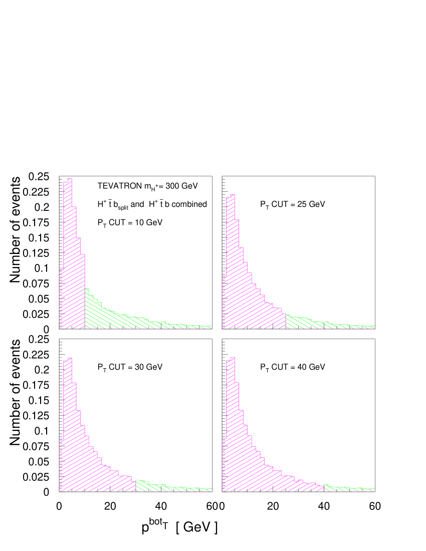
Figure 5: Transverse momenta distribution of the $b$-quark sewn for various values of $p_{T}^{cut}$ for the $pp(\bar{b}g)\rightarrow H^{+}\bar{t}+b_{split}$ and $pp(gg)\rightarrow H^{+}\bar{t}b$ processes at the Tevatron for $M_{H^{+}}=300\,{\rm GeV}$.

3.5 Kinematical analysis

As we mentioned, the $b\bar{b}b(\bar{b})+\ell^{\pm}+2jets+p_{T}^{miss}$ signature of signal and background processes is the subject of this study. One should reconstruct the $t\bar{t}b(\bar{b})$ state from this signature and then, the charged Higgs boson mass from all possible combinations of $tb$-invariant masses. At the same time one should work out an efficient set of kinematical cuts for the background suppression.

For reconstructing the $t\bar{t}b(\bar{b})$ final state, we follow the procedure described below.

• We reconstruct the W-boson mass from lepton and neutrino momenta: $M_{W1}^{rec}=(p_{\ell}+p_{\nu})^{2}$. The basic cuts for the lepton (electron or muon) has been chosen as follows:

  $$p_{T}^{\ell}>15\,{\rm GeV},\,\,\,\,\,\,\,\,|\eta_{\ell}|<2.5,\,\,\,\,p_{T}^{miss}>15\,{\rm GeV}\,\,.$$ (17)

  To find the $p_{z}$ of neutrino and therefore the neutrino 4-momentum, one should solve the quadratic equation $m_{\ell\nu}=M_{W}$, which can have two solutions. We reject events if this equation has no solutions, while in case it has two solutions we keep both of them.

• We reconstruct the mass of the second W-boson ($M_{W2}^{rec}$): we keep all dijet combinations for the moment: the effects of the initial- and final-state radiation and $b$-miss-tagging, the number of light jets is almost always larger than two. The following basic cuts for the jets were chosen:

  $$p_{T}^{j,b}>20\,\,(30)\,{\rm GeV}\,\,[\mbox{Tevatron(LHC)}]\,\,\,\,,\,\,\,\,|\eta_{j}|<3,\,\,|\eta_{b}|<2\,.$$ (18)

• Then we form and keep all $m_{t_{1}}=M_{W1b}$ and $m_{t_{2}}=M_{W2b}$ combinations for the first and second top-quarks.

• In the final step we form the $\chi$ function

  $$\chi=\sqrt{(M_{W1}^{rec}-M_{W})^{2}+(M_{W2}^{rec}-M_{W})^{2}+(m_{t_{1}}-m_{t})^{2}+(m_{t_{2}}-m_{t})^{2}}$$ (19)

  for all combinations of $b$-jets, jets, lepton and neutrino and choose the combination giving the smallest (best) value of the $\chi$ function. The optimized value of the cut on the $\chi$ function was found to be

  $$\chi<\chi_{max}=100\,{\rm GeV}\,\,\mbox{at the Tevatron},\,\,\,\,\chi<\chi_{max}=60\,{\rm GeV}\,\,\mbox{at the LHC}\,.$$ (20)

It should be noted that the reconstruction thus made is independent of the order in which $M_{W1}^{rec},M_{W2}^{rec},m_{t_{1}}$, $m_{t_{2}}$ were formed. This leads to a better signal efficiency, a better probability of a correct reconstruction and a better control of the efficiency through the only relevant parameter, $\chi_{max}$. At the Tevatron, the cut on $\chi$ is quite relaxed by the lack of statistics, while at the LHC this cut could be tightened further, gaining both signal/background ($S/B$) ratio and significance ($S/\sqrt{B}$).

After the reconstruction of the $t\bar{t}b\bar{b}$ state one should reconstruct the charged Higgs boson mass for the signal and the continuous $tb$ mass for the background. We assume that the $b$-jet with the highest $p_{T}$ in $\bar{t}bt(\bar{b})$ signature comes from the $H^{+}$ decay. The probability of that being correct is directly related to the value of $M_{H^{+}}$: for $M_{H^{+}}\simeq 200\,{\rm GeV}$ it is only about 50% while for $M_{H^{+}}\simeq 300\,{\rm GeV}$ the $b$-jet coming from the $H^{+}$ decay has the highest $p_{T}$ in already 75% of the cases. Since we chose just one $b$-jet, there will be two $tb$-invariant mass combinations with two top-quarks that will enter the $m_{tb}$ invariant mass plot.

Like in Ref. [64], we found that $p_{T}^{b}$ from $H^{+}\rightarrow t\bar{b}$ decay is a good variable for the separation of signal from background. However, instead of the fixed $p_{T}^{b}$ cut we apply here the $M_{H^{+}}$-dependent $p_{T}^{b}$ cut:

$$p_{T}^{b}>[M_{H^{+}}/5-15]\,{\rm GeV}\,,$$ (21)

since the peak of this $b$-jet distribution is just proportional to $M_{H^{+}}$. This $M_{H^{+}}$ dependence of the $p_{T}^{b}$ cut allows us to increase the efficiency of the kinematical cut and selection for the signal. The cut depends on the Higgs mass and should be understood as the cut chosen with the respect to the mean value of the mass window where we are looking for the Higgs signal. After the fitting of the Higgs mass using the ’rough’ $p_{T}^{b}$, cut value, one can use the fitted Higgs mass as the input for $p_{T}^{b}(M_{H^{+}})$.

The window around the selected values of $M_{H^{+}}$ was also chosen $M_{H^{+}}$-dependent:

$$|m_{tb}-M_{H^{+}}|<5\sqrt{M_{H^{+}}}\,\,.$$ (22)

One could think of an additional set of kinematical cuts, such as the correlation angle between the Higgs boson direction and its decay products (in the Higgs boson rest frame), the angle between top and bottom from Higgs boson decay (since they tend to be more back-to-back). It turns out that already at the PYTHIA simulation level the difference in those distributions between signal and background is quite blurred. The application of the respective cuts would lead to some increase of the $S/B$ ratio, but at the same time to a definite decrease of the significance and of the accuracy of the signal cross-section measurement.

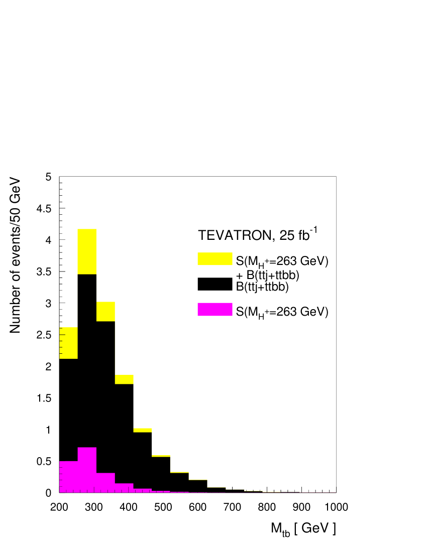
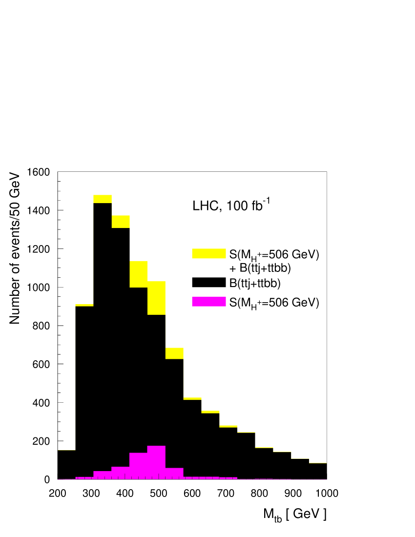
Figure 6: Reconstructed $tb$ invariant-mass distribution for signal, background and signal plus background events, for a) $M_{H^{+}}=263\,{\rm GeV}$ ($M_{A^{0}}=250\,{\rm GeV}$), at the Tevatron and b) $M_{H^{+}}=506\,{\rm GeV}$ ($M_{A^{0}}=500\,{\rm GeV}$), at the LHC, $K^{\rm QCD}=1$.

After all cuts are set up we are ready to present signal and background efficiencies, $S/B$ ratio and significance. The results are summarized in Tables 4 and 5 for the Tevatron and the LHC respectively. We present there the number of signal (2)-(4) $[S]$ events and of background (Table 3) $[B]$ events, as well as their ratio and significance after the reconstruction procedure, $b$-tagging (15)-(16) and set of cuts (17)-(22). Numbers are given for $\tan\!\beta=50$ for an integrated luminosity of $L\equiv\int\mathcal{L}dt=25~{}{\rm fb}^{-1}$ at the Tevatron and an integrated luminosity of $100~{}{\rm fb}^{-1}$ at the LHC. The number of signal events corresponds the tree-level cross-section ($K^{\rm QCD}=1$). Tables 4-5 also present the various efficiencies ($\epsilon$) of the cuts (17)-(22) and reconstruction (including $b$-tagging) for the signal and backgrounds. The last columns of these tables give the 95% C.L. (resp. $5\sigma$) discovery limits of the total signal cross-section in femtobarns (resp. picobarns) for a $25~{}{\rm fb}^{-1}$ (resp. $100~{}{\rm fb}^{-1}$) of total integrated luminosity for the given efficiencies at the Tevatron (resp. LHC).

As an example, Figure 6 shows the reconstructed $tb$ invariant-mass distribution for signal and background events at the Tevatron and the LHC. Owing to the much higher signal rate, the significance of the signal at the LHC is considerably higher than at the Tevatron. In addition, the difference in shape of the signal and background distributions could be clear only for $M_{H^{+}}>400\,{\rm GeV}$, which will be accessible only at the LHC.

$M_{H^{+}}$(GeV)	$S$	$B$	$S/B$	$S/\sqrt{B}$	$\epsilon_{signal}(\%)$	$\epsilon_{ttbb}(\%)$	$\epsilon_{ttj}(\%)$	95% C.L. (fb)
215	9.8	14.0	0.70	2.62	7.10	6.20	0.060	7.50
263	3.5	7.7	0.46	1.27	7.70	3.10	0.034	5.39
310	1.6	7.7	0.21	0.58	8.90	3.10	0.034	4.66
359	0.7	6.4	0.10	0.26	9.20	2.70	0.028	4.29

Table 4: Number of signal (2)-(4) $[S]$ and background –Table 3– events $[B]$, their ratio and significance after reconstruction procedure, $b$-tagging (15)-(16) and set of cuts (17)-(22) at the Tevatron. The last column gives the 95$\%$ C.L. discovery limit ($\sim 2\,\sigma$) on the total signal cross-section in femtobarns for $25~{}{\rm fb}^{-1}$ of total integrated luminosity and given efficiencies. See text for details. $K^{\rm QCD}=1$.

$M_{H^{+}}$(GeV)	$S$	$B$	$S/B$	$S/\sqrt{B}$	$\epsilon_{signal}(\%)$	$\epsilon_{ttbb}(\%)$	$\epsilon_{ttj}(\%)$	$5\sigma$(pb)
215	847	1490	0.57	21.9	0.32	0.29	0.005	1.02
310	2386	5890	0.41	31.1	2.00	1.25	0.018	0.32
408	1560	6210	0.25	19.8	2.70	1.50	0.016	0.25
506	773	3770	0.21	12.6	2.60	0.97	0.009	0.20
605	433	2070	0.21	9.5	2.60	0.56	0.004	0.15
704	217	1170	0.19	6.3	2.30	0.33	0.002	0.13
804	117	666	0.18	4.5	2.10	0.19	0.001	0.10

Table 5: Number of signal (2)-(4) $[S]$ and background –Table 3– events $[B]$, their ratio and significance after reconstruction procedure, $b$-tagging (15)-(16) and set of cuts (17)-(22) at the LHC. The last column gives the 5$\sigma$ discovery limit on the total signal cross-section in picobarns for $100~{}{\rm fb}^{-1}$ of total integrated luminosity and given efficiencies. See text for details. $K^{\rm QCD}=1$.

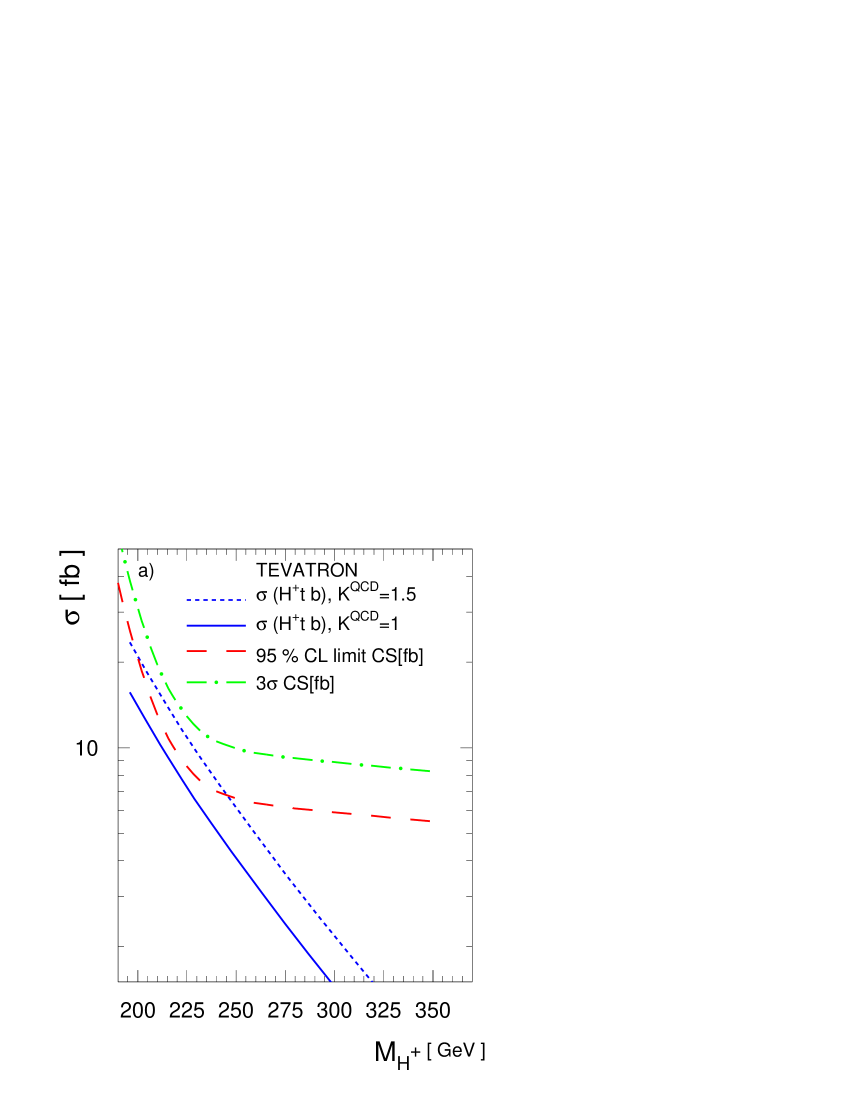
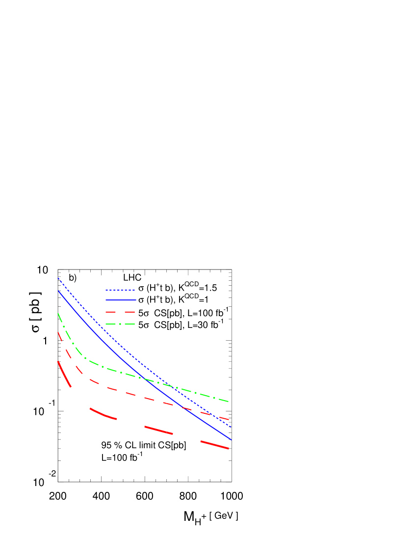
Figure 7: The total cross-section $\sigma(p\bar{p}(pp)\to H^{+}\bar{t}b+X)$ for fixed $\tan\!\beta=50$ including a QCD factor $K^{\rm QCD}=1$ (solid) and $K^{\rm QCD}=1.5$ (dotted): a) at the Tevatron, dashed and dot-dashed lines correspond to the cross-section values necessary for the $2\sigma$ ($95\%$ C.L.) exclusion and the $3\sigma$ evidence respectively, at the integrated luminosity $L=25~{}{\rm fb}^{-1}$; b) at the LHC, dot-dashed and dashed lines corresponding to the cross-section necessary for the $5\sigma$ discovery at the integrated luminosity $L=30~{}{\rm fb}^{-1}$ and $100~{}{\rm fb}^{-1}$ respectively; the long-dashed line at the bottom corresponds to the $95\%$ C.L. limit at $L=100~{}{\rm fb}^{-1}$.

In spite of the fact that the S/B ratio is quite high at the Tevatron for $M_{H^{+}}=215\,{\rm GeV}$, the signal rate itself is small, even for $\tan\!\beta=50$. That is why we try to keep the signal efficiency as high as possible by relaxing the acceptance cut on $p_{T}^{j,b}$ and the cut on $\chi$. Table 4 shows that at the Tevatron there is no $5\,\sigma$ discovery limit available for Higgs boson masses above $200\,{\rm GeV}$, although there is a narrow window $(175-195)\,{\rm GeV}$ for Higgs boson masses just above the kinematical limit for the top quark decay into a charged Higgs boson. In general, however, at the Tevatron one can only hope to exclude charged Higgs boson masses up to the certain value defined by the efficiencies, the value of $\tan\beta$ (and the other MSSM parameters beyond the tree level) and the total integrated luminosity. Even the exclusion region is apparently small. The signal significance is only $3.4$ for the charged Higgs boson with mass $215\,{\rm GeV}$, $\tan\beta=50$ and $K$-factor $K^{\rm QCD}=1.5$. For this value of $\tan\!\beta$ the 95% C.L. limit on the charged Higgs boson mass is $240\,{\rm GeV}$. We use the Poisson statistics when putting this limit at the Tevatron, since the number of events is small for both the signal and the background. On the other hand, for $K^{\rm QCD}\leq 1$ it is not possible to obtain any limits using this channel, as it is obvious from the comparison of Tables 1 and 4.

At the LHC, the situation is much better, with higher luminosity ($30-300~{}{\rm fb}^{-1}$) and a signal rate higher by 3 orders of magnitude with respect to the Tevatron. Here we can allow ourselves to use the tighter kinematical cuts (17)-(20). We try to reach the best significance ratio $S/\sqrt{B}$ while keeping the $S/B$ ratio above the 10% level. Based on the efficiencies of Table 5, we find that a charged Higgs boson can be discovered at the $5\sigma$ level, with mass up to about $900\,{\rm GeV}$ for $\tan\!\beta=50$ and $K^{\rm QCD}=1.5$.

It is important also to understand the role of the $K$-factor. In Fig. 7 we present the cross-section for the $p\bar{p}(pp)\to H^{+}\bar{t}b+X$ process for $K^{\rm QCD}=1.5$ and $K^{\rm QCD}=1$ (dotted and solid lined, respectively), and the cross-section for necessary for the discovery/exclusion of a charged Higgs boson. In Fig. 7a we show the $95\%$ C.L. limit (dashed) and the $3\sigma$ evidence cross-section at the Tevatron for an integrated luminosity of $25~{}{\rm fb}^{-1}$. Fig. 7b shows the cross-section for the $5\,\sigma$ discovery (i.e. $5\,\sqrt{B}$) at the LHC for an integrated luminosity of $L=30~{}{\rm fb}^{-1}$ (corresponding to $3$ years of low-luminosity regime) and $100~{}{\rm fb}^{-1}$ ($1$ year high-luminosity regime). Notice that the discovery curves also evolve with $M_{H^{+}}$ because the efficiencies are $M_{H^{+}}$-dependent (see Tables 4 and 5). Even at low luminosity, the $5\,\sigma$ discovery limit for the LHC is $600\,{\rm GeV}$ for $K^{\rm QCD}=1$, $700\,{\rm GeV}$ and for $K^{\rm QCD}=1.5$. Of course, if the $K^{\rm QCD}$ factor turns out to be below 1, the mass reach is lowered accordingly, e.g. $450\,{\rm GeV}$ for $K^{\rm QCD}=0.5$. One can see that the value of the $K$-factor is really important because a variation of $K^{\rm QCD}$ from $1$ to $1.5$ causes a $100\,{\rm GeV}$ shift of the limit on the charged Higgs boson mass. For $L=100~{}{\rm fb}^{-1}$ the discovery limit is $790\,{\rm GeV}$ if $K^{\rm QCD}=1$, and $900\,{\rm GeV}$ for $K^{\rm QCD}=1.5$ ($600\,{\rm GeV}$ for $K^{\rm QCD}=0.5$). In this figure we also show the $2\,\sqrt{B}$ curve, from which one obtains immediately that the charged Higgs boson can be excluded at the $95\%$ C.L. up to a mass of about $1\,{\rm TeV}$ even for $K^{\rm QCD}=1$ at $100~{}{\rm fb}^{-1}$ of integrated luminosity. In Section 4 we shall come back to this figure and we will show that there are regions of the MSSM parameter space where the total effective $K^{\rm MSSM}$ factor in eq.(14) could be $\sim(40-50)\%$ larger than the typical $K$-factor expected from pure QCD alone.

One can assume that systematic uncertainties due to the parton distribution uncertainties as well as to the uncertainty from the higher-order QCD corrections for the background (or from a choice of the QCD scale for the background) could be significantly reduced by normalizing the MC $tb$ distribution to the data. Under the assumption that normalization to the data will reduce systematic uncertainties up to the level of $7\%$, one can also estimate the accuracy of the measurement of the signal cross-section using efficiencies from Table 5. For example, for $M_{H^{+}}=408\,{\rm GeV}$ the accuracy of the cross-section measurement will be:

$$\frac{\delta S}{S}=\frac{\sqrt{(\sqrt{B})^{2}+\delta B_{syst}^{2}}}{S}=\frac{\sqrt{6210+(0.07\times 6210)^{2}}}{1560}\simeq 28\%$$ (23)

This means that $H^{+}\bar{t}b$ coupling could be measured with an accuracy of $(1/2)\delta S/S\simeq 14\%$. In the next section we show that the SUSY corrections could be substantially higher than $14\%$, therefore being potentially measurable!

4 The role of the SUSY corrections

4.1 The leading effects. Theoretical discussion

In Section 3 we have concentrated on the results for the cross-section and background for the charged Higgs boson production process (1) without including the various sources of potentially important SUSY corrections. However, in Section 2 we have already warned about the possibility of non-negligible SUSY effects in the signal and we have correctly identified the region of the parameter space where they can be optimized, namely at high $\tan\beta$. It is now time to study this issue in detail because, as we shall see below, the supersymmetric loops can be very sizeable and may play a momentous role in the production of a charged Higgs boson. In fact, they can not only enhance the signal versus the background, but they can also be used as a means to characterize the supersymmetric nature of the charged Higgs boson potentially found in hadron colliders through the mechanism (1).

Among the plethora of possible SUSY corrections we disregard virtual supersymmetric effects on the $gqq$ and $ggg$ vertices and on the gluon propagators. We expect those to be of order $(\alpha_{S}/4\pi)\cdot(s/M_{SUSY}^{2})$ and thus suppressed by a non-enhanced (i.e. $\tan\!\beta$-independent) MSSM form factor coming from the loop integrals. Therefore, we can neglect these contributions as we are only considering effects of the form $(\alpha_{S}/4\pi)^{n}\cdot\tan^{n}\beta$ at large $\tan\!\beta$ . As previously emphasized, the cross-section for the signal increases steeply with $\tan\!\beta$ (see Fig. 3) and becomes highly significant for $\tan\!\beta$$>30$, while it is much smaller for $\tan\!\beta$ in the low interval $2-20$ where the remaining SUSY corrections are of the same order or even dominant, so our approximation is well justified. Similarly, we neglect all those electroweak corrections in vertices and self-energies which are proportional to pure $SU(2)_{L}\times U(1)_{Y}$ gauge couplings; in particular, vertices involving electroweak gauge bosons and those involving electroweak gauginos. Furthermore, we have checked that vertices involving Higgs bosons exchange yield a very tiny overall contribution, due to automatic cancellations arranged by the underlying supersymmetry. Finally, there are the strong gluino-squark diagrams and the $\tan\beta$-enhanced higgsino-squark vertices implicit in chargino-neutralino loops. We have extracted (see below) the parts of these interactions which are (by far) the more relevant ones at high $\tan\beta$ and confirmed that the remaining contributions are negligible. In practice this means that we will concentrate our analysis on the interval $\tan\beta>20$ where we can be sure that our approximation does include the bulk of the MSSM corrections while at the same time the cross-section of process (1) starts to be sufficiently large to consider it as an efficient mechanism for charged Higgs boson production (Cf. Fig. 3). To be more precise, we shall hereafter confine our study of process (1) to within the relevant interval $20<\tan\!\beta<60$, where the upper limit on $\tan\!\beta$ is approximately fixed by the condition of perturbativity of the Yukawa couplings.

As a consequence we can just concentrate on the leading quantum effects. The latter can be conveniently described through an effective Lagrangian approach that contains effective couplings absorbing both the leading SUSY contributions and the known part of the QCD corrections [35]. At high $\tan\beta$ the most relevant piece is the effective $tbH^{+}$-coupling as it carries the leading part of the quantum effects. Indeed, on the one hand the quantity $\Delta m_{b}$ in (13) contains the bulk of the supersymmetric contributions. On the other by trading the bottom quark mass by the corresponding running quantity one can also include a sizeable part of the QCD effects, namely the (universal) renormalization group effects. As a result the relevant piece of the effective Lagrangian at high $\tan\beta$ involving the $tbH^{+}$ vertex can be cast as follows:

$$\mathcal{L\,}\mathbb{=\,}\frac{gV_{tb}}{\sqrt{2\,}M_{W}}\,\frac{\overline{m}_{b}(\mu_{R})\,\tan\beta}{1+\Delta m_{b}}\,H^{+}\overline{t}_{L}\,b_{R}+h.c.$$ (24)

where $\mu_{R}$ is the renormalization scale for the bottom quark running mass $\overline{m}_{b}(\mu_{R})$ at the NLO in the $\overline{MS}$ scheme. One usually assigns a value to $\mu_{R}$ given by the characteristic energy scale of the process under consideration. In our case (Cf. Fig. 1) it would be natural to set $\mu_{R}=m_{t}+M_{H^{+}}$. However, following the discussion in Section 2, we will use the (on-shell) pole quark masses in the tree-level cross-section, and will parameterize the QCD corrections by means of a $K^{\rm QCD}$-factor.

On the SUSY side the effects encoded in $\Delta m_{b}$ are related to the bottom mass counterterm $\delta m_{b}$ in the on-shell scheme. If $m_{b}$ is the pole mass, then its relation with the corrections resummed into the bottom quark Yukawa coupling leads to the consistency formula

$$m_{b}+\delta m_{b}{=}\frac{m_{b}}{1+\Delta m_{b}}\,;$$ (25)

in particular $\Delta m_{b}=-\,\delta m_{b}/m_{b}$ at one loop. The SUSY effects on $\Delta m_{b}$ can be of two types, SUSY-QCD and SUSY-EW. The strong part of $\Delta m_{b}$ originates from finite corrections induced by mixed LH and RH weak-eigenstate sbottoms and gluino loops [10, 33] (Fig. 8a):

$$\left(\Delta m_{b}\right)_{\mathrm{SUSY-QCD}} =-\,C_{F}{\frac{\alpha_{S}(M_{\mathrm{SUSY}})}{2\pi}}\,m_{\tilde{g}}\,M_{LR}^{b}\,I(m_{\tilde{b}_{1}},m_{\tilde{b}_{2}},m_{\tilde{g}})$$

$$\rightarrow+{\frac{2\alpha_{S}(M_{\mathrm{SUSY}})}{3\pi}}\,m_{\tilde{g}}\,\mu\,\tan\beta\,I(m_{\tilde{b}_{1}},m_{\tilde{b}_{2}},m_{\tilde{g}})\,,$$ (26)

where $C_{F}=(N_{c}^{2}-1)/2N_{c}=4/3$ is a color factor (with $N_{c}=3$). Moreover we have $\alpha_{S}(M_{\mathrm{SUSY}})\simeq 0.09$, $M_{LR}^{b}=A_{b}-\mu\,\tan\beta$ and the last expression in (26) holds only for sufficiently large $\mu\,\tan\beta\gg A_{b}$. Here $\mu$ is the higgsino mass parameter in the superpotential, and should not be confused with the renormalization scale $\mu_{R}$. Finally, $A_{b}$ is the bottom quark trilinear coupling in the soft-SUSY-breaking part of the superpotential. As for the electroweak effects on $\Delta m_{b}$ they stem from similar loops involving mixed LH and RH-stops and mixed charged higgsinos $\tilde{H}_{1}-\tilde{H}_{2}$ and read (Fig. 8b)

$$\left(\Delta m_{b}\right)_{\mathrm{SUSY-Yukawa}} =+{\frac{h_{t}\,h_{b}}{16\pi^{2}}}\,\,{\frac{\mu}{m_{b}}}\,m_{t}\,M_{LR}^{t}I(m_{\tilde{t}_{1}},m_{\tilde{t}_{2}},\mu)$$

$$\rightarrow+{\frac{Y_{t}}{4\pi}}\,A_{t}\,\,\mu\,\tan\beta\,\,I(m_{\tilde{t}_{1}},m_{\tilde{t}_{2}},\mu)\,\,.$$ (27)

Here $A_{t}$ is the top quark counterpart of $A_{b}$; we have defined $Y_{t}=h_{t}^{2}/4\pi\simeq 1/4\pi$ and $M_{LR}^{t}=A_{t}-\mu\cot\beta$, and again the last expression holds for large enough $\tan\beta$ only. Gaugino-higgsino ($\tilde{W}-\tilde{H}_{2}$) mixing also contributes with $\tan\!\beta$ enhanced terms to $\Delta m_{b}$ (Fig. 8c):

Figure 8: Leading contributions to $\Delta m_{b}$ – eq. (25). a) SUSY-QCD contributions (26); b) SUSY-Yukawa contributions (27); c) SUSY-EW gauge contributions (28). Each cross represents a mass-insertion; each cross with a circle represents a field mixing term in the electroweak eigenstate basis for squarks or gaugino-higgsinos.

$$\left(\Delta m_{b}\right)_{\mathrm{SUSY-gauge}}=- \frac{g^{2}}{16\pi^{2}}\mu\tan\!\beta M_{2}\bigg{[}\cos^{2}\theta_{\tilde{t}}\,I(m_{\tilde{t}_{1}}^{2},M_{2}^{2},\mu^{2})+\sin^{2}\theta_{\tilde{t}}\,I(m_{\tilde{t}_{2}}^{2},M^{2}_{2},\mu^{2})\,$$

$$+\frac{1}{2}\left(\cos^{2}\theta_{\tilde{b}}\,I(m_{\tilde{b}_{1}}^{2},M_{2}^{2},\mu^{2})+\sin^{2}\theta_{\tilde{b}}\,I(m_{\tilde{b}_{2}}^{2},M^{2}_{2},\mu^{2})\right)\bigg{]}\,.$$ (28)

In the above formulae we have introduced the (positive-definite) three-point function

$$I(m_{1},m_{2},m_{3}) \equiv 16\,\pi^{2}i\,C_{0}(0,0,m_{1},m_{2},m_{3})$$

$$={\frac{m_{1}^{2}\,m_{2}^{2}\ln{\frac{m_{1}^{2}}{m_{2}^{2}}}+m_{2}^{2}\,m_{3}^{2}\ln{\frac{m_{2}^{2}}{m_{3}^{2}}}+m_{1}^{2}\,m_{3}^{2}\ln{\frac{m_{3}^{2}}{m_{1}^{2}}}}{(m_{1}^{2}-m_{2}^{2})\,(m_{2}^{2}-m_{3}^{2})\,(m_{1}^{2}-m_{3}^{2})}}\,.$$ (29)

This function is well defined even when all masses are equal, which is precisely the situation where it attains its minimum. Thus, if we roughly assume that all masses are equal to $M_{SUSY}$, it boils down to

$$I(m_{i}=M_{SUSY})=\frac{1}{2\,M_{SUSY}^{2}}\,.$$ (30)

Furthermore, by setting $\left|\mu\right|=\,m_{\tilde{g}}=M_{SUSY}$ and $\tan\beta=50$ one immediately sees that eq.(26) gives a large correction of $\pm\mathcal{O}(50\%)$ depending on the sign of $\mu$. Notice that in the on-shell renormalization scheme defined in [10], the SUSY-EW gauge contributions from eq. (28) are compensated for by those equivalent to Fig. 8c but with a external $\tau$-lepton and sneutrinos/$\tau$-sleptons circulating in the loop. However the resummation in (24) can only be done in a mass-independent renormalization scheme [35], and the diagrams in Fig. 8c must be taken into account. The difference between the two renormalization schemes amounts to a finite shift in the definition of $\tan\!\beta$ which, however, is not significant in the interesting region $\tan\!\beta\gg 1$.

Of course, the top quark Yukawa coupling receives $\Delta m_{t}$ corrections which are the counterpart to those for the bottom quark, eqs. (26)-(28), but they are suppressed (rather than enhanced) by $\tan\!\beta$ and so they will be ignored.

It should be emphasized that both types of SUSY contributions to $\Delta m_{b}$ can be sizeable; naively one could think that the SUSY-EW contributions induced by higgsino-gaugino exchange are suppressed with respect to the (gluino induced) SUSY-QCD contribution by a factor of $\alpha_{W}/\alpha_{S}\sim 10^{-2}$, but this is not necessarily so. In fact, in regions of the parameter space where the $3$-point functions on the RHS of (26) and (27) are approximately equal  the two types of corrections are roughly of order $\alpha_{S}\,\,\mu\,\tan\beta/M_{SUSY}$ and $Y_{t}\,\mu\,\tan\beta/M_{SUSY}$ respectively, and since $\alpha_{S}\simeq Y_{t}$ they should be comparable. However, from a more accurate estimation including the color factor $C_{F}$ the ratio between the SUSY-QCD and SUSY-EW effects yields

$$\frac{8}{3}\left(\frac{\alpha_{S}}{Y_{t}}\right)\left(\frac{m_{\tilde{g}}}{A_{t}}\right)\simeq 3\,\left(\frac{m_{\tilde{g}}}{A_{t}}\right)\,.$$ (31)

This ratio can be smaller than $1$ if $A_{t}\gtrsim 3\,m_{\tilde{g}}$. However in the numerical analysis below we typically choose $m_{\tilde{g}}>A_{t}$ (Cf. Table 6), and this makes the SUSY-QCD effects generally dominant. There are indeed reasons to envision this kind of scenario. First, the gluino mass is expected to be rather large, of the order of $1\,{\rm TeV}$. Second, we cannot choose $A_{t}$ too large, say above $1\,{\rm TeV}$, because this could disrupt the $SU(3)_{c}$ and $U(1)_{em}$ symmetries of the electroweak vacuum state. An approximate necessary condition for this not to happen is [72]

$$A_{t}^{2}<3\,(M_{Q}^{2}+M_{U}^{2}+M_{H_{2}}^{2}+\mu^{2})\,.$$ (32)

Here $M_{Q,U}$ are the LH and RH stop SUSY-breaking mass parameters, $M_{H_{2}}^{2}$ (with $M_{H_{2}}^{2}<0$, due to the radiative breaking of the gauge symmetry) is the soft-SUSY-breaking mass associated to the $H_{2}$ doublet (the one that couples the top quark) and $\mu$ is again the supersymmetric higgsino mass parameter. In a typical scenario where $m_{\tilde{g}}$ is larger than any squark mass and any electroweak mass parameter, one may assume $A_{t}\lesssim M_{Q,U}\lesssim m_{\tilde{g}}$ (Cf. Table 6). In this case the RHS of eq.(31) should be greater than $1$ and the SUSY-QCD effects are dominant. Third, these effects have the remarkable property that they decouple very slowly with the gluino mass [10]. Indeed, for sbottom masses of a few hundred $\mathrm{GeV}$ the gluino mass can be as high as $1\,{\rm TeV}$ and the correction is still of order $(20-30)\%$. This is due to the helicity flip in the gluino line which generates the gluino mass term in the numerator of eq.(26). For $m_{\tilde{g}}\sim 1\,{\rm TeV}$ it would be contrived to assume $A_{t}>3\,m_{\tilde{g}}$, and hence the SUSY-EW effects must surely have gone away in the heavy gluino regime while the strong supersymmetric effects can still remain. Of course the correction (26) eventually dies out with $m_{\tilde{g}}$, but very slowly. Notice that in the opposite limit, $m_{\tilde{g}}\rightarrow 0$, the SUSY-QCD effects (26) also tend to zero and one is left with the subleading SUSY-QCD contributions from the renormalized three-point functions. We shall not focus on the light gluino case here, although in practice it is equivalent to assume that the bulk of the SUSY corrections is just given by the electroweak part (26), which can still be rather substantial. These remarks show that the leading type of SUSY effects on our process can have different origin and remain significant in large portions of the MSSM parameter space.

Ultimately the origin of the exceptional SUSY quantum effects (26) and (27) stems from the breaking of SUSY through dimensional soft terms like gaugino masses and trilinear couplings, and therefore they cannot be described – unlike the conventional QCD effects considered before – through the universal renormalization group running of the parameters. Technically, they are finite threshold effects which must be included explicitly at energies above $M_{SUSY}$, the characteristic SUSY breaking scale at low energies [33].

Remarkably, the finite threshold effects do not vanish when the soft-SUSY-breaking parameters, together with the higgsino mass parameter $\mu$, are scaled up simultaneously to arbitrarily large values. This is immediately seen from (26) and (27) by letting simultaneously $\mu\rightarrow\lambda\,\mu$ and $\widetilde{m}\rightarrow\lambda\,\widetilde{m}$ in these equations, where $\lambda$ is an arbitrary dimensionless scale factor and $\widetilde{m}$ is any soft-SUSY-breaking parameter. However, it is important to notice that the apparent non-decoupling behaviour exhibited by this kind of SUSY effects is rendered innocuous after resumming all the corrections of the form $\left(\alpha_{S}\,\,\mu\,\tan\beta/M_{SUSY}\right)^{n}$ and $\left(Y_{t}\,\mu\,\tan\beta/M_{SUSY}\right)^{n}$ to all orders $n=1,2,\ldots$ [35]. The resummed result is indeed given by the effective bottom quark Yukawa coupling (13), which shows that there are no higher order disturbing effects of the form $\Delta m_{b}{}^{n}\sim(\alpha_{S}/4\pi)^{n}\cdot\tan^{n}\beta$ when $\Delta m_{b}\geq 1$ and the expansion

$$\frac{1}{(1+\Delta m_{b})}=1-\Delta m_{b}+\Delta m_{b}{}^{2}-\ldots$$ (33)

is not possible. On the other hand for $\left|\Delta m_{b}\right|\ll 1$ the expansion is of course allowed and the higher order powers $\Delta m_{b}{}^{n}$ give small corrections to the linear approximation $1-\Delta m_{b}$ used in [10]. However, for $\left|\Delta m_{b}\right|\lesssim 1$ and $\Delta m_{b}<0$ the resummed SUSY contribution is seen to substantially reinforce the one loop result. For example, if $\Delta m_{b}=-50\%$, the one-loop correction is $+50\%$ whereas the resummed result gives a $+100\%$ effect! Therefore, the SUSY radiative corrections can be quite large, and may remain so even for very high values of $M_{SUSY}$, but their resummation is eventually kept under control when $\left|\Delta m_{b}\right|\gg 1$.

The effective Lagrangian approach just outlined is also very useful for the practical calculation of the cross-sections. In fact, by appropriately modifying the MSSM Feynman rules using the effective vertex interactions described above we have managed to automatically generate the leading quantum effects from the CompHEP calculation of the cross-sections.

Although $\Delta m_{b}$ in the above equations is the only correction of order $(\alpha/4\pi)\tan\!\beta$ ($\alpha=\alpha_{S},\alpha_{W}$) that dominates for large $\tan\!\beta$, we have also tested the effect from the off-shell SUSY-QCD and SUSY-EW corrections to the $H^{+}\bar{t}b$ vertex and to the fermion propagators. As already mentioned above, some of these off-shell vertices (in particular those involving chargino-neutralino exchange) carry some $\tan\beta$-enhanced Yukawa couplings that could be important. Nevertheless it turns out that these contributions are not comparable to the leading $\Delta m_{b}$ ones. The point is that the effects entering $\Delta m_{b}$ at high $\tan\beta$ are of the type $\alpha_{S}\tan\beta$ or $Y_{t}\tan\beta$ whereas those from the aforementioned vertices are of the type $\left(g\,m_{b}\,\tan\beta/M_{W}\right)^{2}/4\pi\sim Y_{t}$, and so they are down by an extra power of $\tan\beta$. At the end of the day they are subleading effects on equal footing to the previously dismissed SUSY corrections to pure QCD vertices. Actually, to have full control on the quantitative size of these effects we have explicitly checked that their numerical contribution is immaterial. To this end we have evaluated the full set of one-loop SUSY diagrams for the relevant $tbH^{+}$ vertex. The same set was considered in detail Ref.[10] in the case where all external particles are on-shell. In the present case, however, at least one of the quarks in that vertex is off shell (see Fig. 1). Therefore, we can use the same bunch of diagrams as in the on-shell case but we have to account for the off-shell external lines, which is a non-trivial task. We have studied this issue in detail by expanding the off-shell propagators

$$\frac{1}{(p+q)^{2}-M^{2}}=\frac{1}{q^{2}-M^{2}}\left[1-\frac{p^{2}+2pq}{q^{2}-M^{2}}+\left(\frac{p^{2}+2pq}{q^{2}-M^{2}}\right)^{2}+\ldots\right]$$ (34)

in the expression of the one-loop functions. The result is that the off-shell corrections are generally small for they are of order or below the non-leading one-loop effects that we have neglected. For the computation of the SUSY-corrected matrix elements we have proceeded in the following way: first, we have modified CompHEP’s Feynman rules to allow for the most general $\bar{t}bH^{+}$ vertex; then we have let CompHEP reckon the squared matrix elements and dump the result into REDUCE code. At this point, we have inserted expressions for the coefficients of the off-shell $\bar{t}bH^{+}$ vertex that include the one-loop off-shell supersymmetric corrections to the vertex itself and to the off-shell fermion propagators and fermionic external lines. Only half the renormalization of an internal fermion line has to be included, the other half being associated to the $gqq$ vertex. Higher order terms not included in the effective Lagrangian (24) have been discarded. The subsequent numerical computation of the one-loop integrals has been done using the package LoopTools [73]. This procedure has allowed us to estimate the relative size of the off-shell effects in the signal cross-section, whose effects are analyzed in the next section.

The upshot is that the approximation of neglecting $q\bar{q}g$ vertex and propagator corrections in the cross-section computation of process (1), which may be called “improved Born” approximation (see next section), is really justified in the relevant region of parameter space.

4.2 Numerical analysis of the SUSY corrections

We have seen above that the SUSY corrections are potentially large and can be of both signs. The leading correction to the cross-section of our process (1) goes roughly as $\sigma\rightarrow\sigma(1-2\Delta m_{b})$ at one loop, so that the sign of the SUSY-QCD part carries just the sign of $-\mu$ whereas the SUSY-EW one depends on the sign of the combined parameter $-\mu A_{t}$. Recall that the radiative B-meson decays (based on the $b\rightarrow s\,\gamma$ transition) prefer the sign $\mu A_{t}<0$ (see e.g Refs. [20, 74]) if the charged Higgs boson is not exceedingly heavy. The reason is that if stops and charginos are of similar mass to that of the Higgs boson then they can compensate for the Higgs boson contribution, which by itself would overshoot the experimentally allowed range for $BR(b\rightarrow s\,\gamma)$. In this case the $\mu A_{t}<0$ sector of the MSSM parameter space offers the Tevatron II a chance to observe a supersymmetric charged Higgs boson of around $200\,{\rm GeV}$. For a much heavier Higgs boson, however, namely that accessible only to LHC, $b\rightarrow s\,\gamma$ does not place any restriction on the sign of $\mu\,A_{t}$.

Obviously there is a preferred sign for our process: the optimal situation for the charged Higgs boson production mechanism (1) to be maximally sensitive to the SUSY effects is when $\mu<0$ and $A_{t}>0$ corresponding to both corrections, SUSY-QCD and SUSY-EW, giving a positive contribution to the cross-section. The next-to-interesting case is when $\mu<0$ and $A_{t}<0$. Here the electroweak loops try to balance the SUSY-QCD ones, but the dominance of the latter still leaves a sizeable net outcome – some $60\%$ of the previous case. Of course there is also the odd possibility that $\mu>0$ and $A_{t}>0$, but in this circumstance the SUSY quantum effects could still manifest themselves (if $\tan\!\beta$ is large) through an effective $K$-factor (14) sensibly smaller than the one predicted by QCD expectations: $K^{\rm MSSM}<K^{\rm QCD}$. The worse possible situation would occur if $\tan\beta$ is small, say in the intermediate range $2<\tan\beta<20$, since no positive nor negative effect whatsoever could be detected; in fact, in this case not even the tree-level signal would be available! In the following we are going to concentrate our numerical analysis on the case $\mu<0$ and $A_{t}>0$, which is the one phenomenologically most appealing and therefore defines the scope of the present study.

In Fig. 9 we present the total cross-section as a function of $\tan\!\beta$ at the LHC (with $M_{H^{+}}=500\,{\rm GeV}$) and the Tevatron (with $M_{H^{+}}=250\,{\rm GeV}$) for $K^{\rm QCD}=1$. We show the tree-level result and four additional cases that include SUSY corrections: they correspond to the four sets of parameters displayed in Table 6. The SUSY-corrected curves contain all the known corrections discussed in the previous section, including the resummation of the SUSY effects. As can be seen the numerical effect of the SUSY contributions can be dramatic; for the Set A there is a 100% positive enhancement of the cross-section. However the fact that we have resummed all the leading terms of the form $(\alpha\tan\!\beta)^{n}$ ensures that the prediction is robust under the inclusion of additional higher order effects.

Let us comment briefly on the treatment of the strong structure constant $\alpha_{S}$. We have used the SM value of $\alpha_{S}(Q)$ for the gluon-gluon and quark-gluon vertices. We have to do so, since the value of $\alpha_{S}$ is related to the determination of the PDFs and moreover the SUSY effects on these vertices are, as we have discussed before, non-leading in our case. However, in order to compute the SUSY corrections, we need to compute $\alpha_{S}(M_{SUSY})$, and it would be a very bad approximation to use the SM value. So we use the MSSM value $\alpha_{S}^{\mathrm{MSSM}}(Q)$ to compute the corrections to the $H^{+}\bar{t}b$ vertex.

	$\tan\!\beta$	$\mu$	$M_{2}$	$m_{\tilde{g}}$	$m_{\tilde{t}_{1}}$	$m_{\tilde{b}_{1}}$	$A_{t}$	$A_{b}$
Set A	50	-1000	200	1000	1000	1000	500	500
Set B	50	-200	200	1000	500	500	500	500
Set C	50	200	200	1000	500	500	-500	500
Set D	50	1000	200	1000	1000	1000	-500	500

Table 6: Sets of SUSY parameters used in the computation of the SUSY-corrections to the charged Higgs boson associated production (all masses and trilinear couplings in GeV).

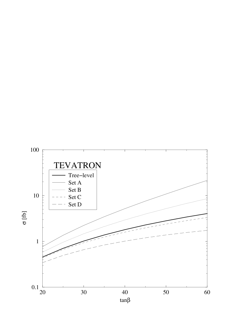
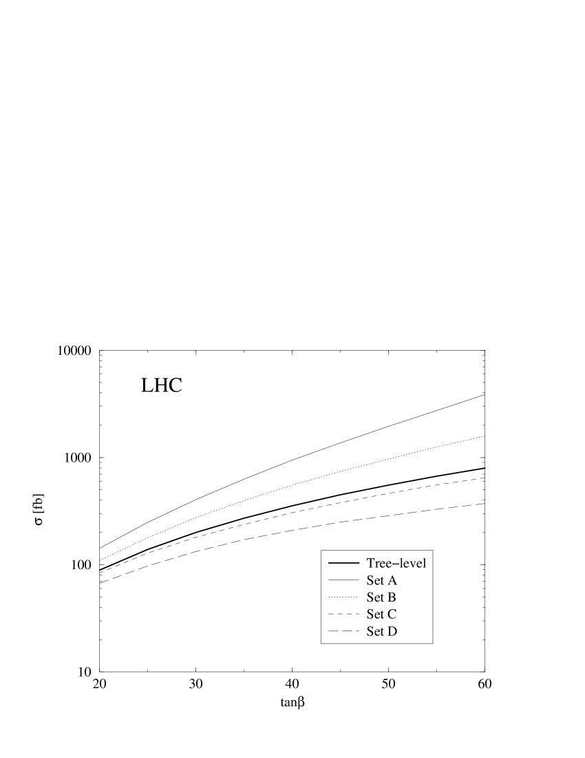
(a)	(b)

Figure 9: Total cross-section for the process $p\bar{p}(pp)\to H^{+}\bar{t}b+X$ as a function of $\tan\!\beta$  in the relevant range of this parameter. The tree-level result and the SUSY-corrected result are shown (with $K^{\rm QCD}=1$) for the four sets of parameters from Table 6, for a) the Tevatron with $M_{H^{+}}=250\,{\rm GeV}$, and b) the LHC with $M_{H^{+}}=500\,{\rm GeV}$.

Of course, one would like to know which is the relative importance of each effect in the final corrected cross-section for the process (1). Let us compare the following set of corrections:

• the full set of SUSY corrections, including resummation and the off-shell two- and three-point functions (labeled Full);

• the corrections including resummation, but using on-shell values for the irreducible three-point functions (On-Shell);

• the one-loop (without resummation) corrections, using also on-shell values for the irreducible three-point functions (OS-nr);

• the tree-level result with the pole quark masses replaced by the effective Yukawa couplings eq. (24) (Improved-Born).

In Fig. 10 we show the total cross-section of process (1) using the four approximations. We use the intermediate Set B of Table 6 which represents a moderate case. The following hierarchy of quantum effects is observed:

$$\sigma({\rm Full)}\stackrel{{\scriptstyle\scriptstyle>}}{{{}_{\sim}}}\sigma({\rm Improved-Born})>\sigma({\rm On-shell})>\sigma({\rm OS-nr})\,.$$ (35)

The effect of the resummation is clearly visible. The difference between the resummed and non-resummed results grows with the magnitude of the corrections; in sets A and D this difference is much larger than that of sets B and C. On the other hand the difference between the Full and the On-Shell results is nearly indistinguishable. So the Off-Shellness effect is generally small in our case and it may be neglected in a first approximation, although it should be taken into account in a detailed study.

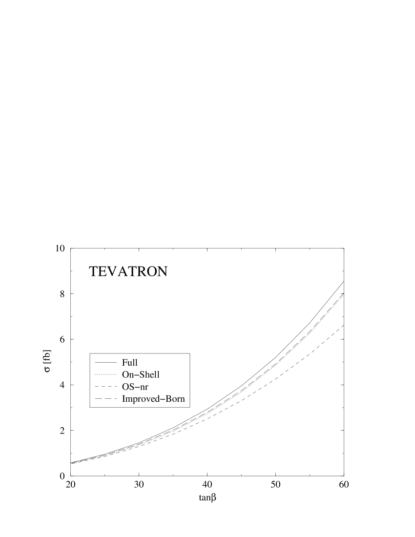
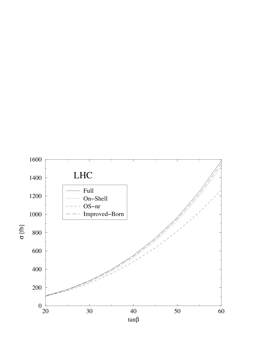
(a)	(b)

Figure 10: As in Fig. 9, but now showing the different approximations described in the text for the intermediate Set B in Table 6, a) for the Tevatron with $M_{H^{+}}=250\,{\rm GeV}$, and b) for the LHC with $M_{H^{+}}=500\,{\rm GeV}$.

In the following we restrict ourselves to plot the effective SUSY $K$-factor ($K^{\rm SUSY}$) involved in the definition (14). This factor embodies the main results of our calculation as it gauges directly the potential impact of the genuine SUSY corrections. It is defined as follows:

$$K^{\mathrm{SUSY}}=\frac{\sigma^{\mathrm{SUSY-corrected}}}{\sigma^{\mathrm{Tree-level}}}\,,$$ (36)

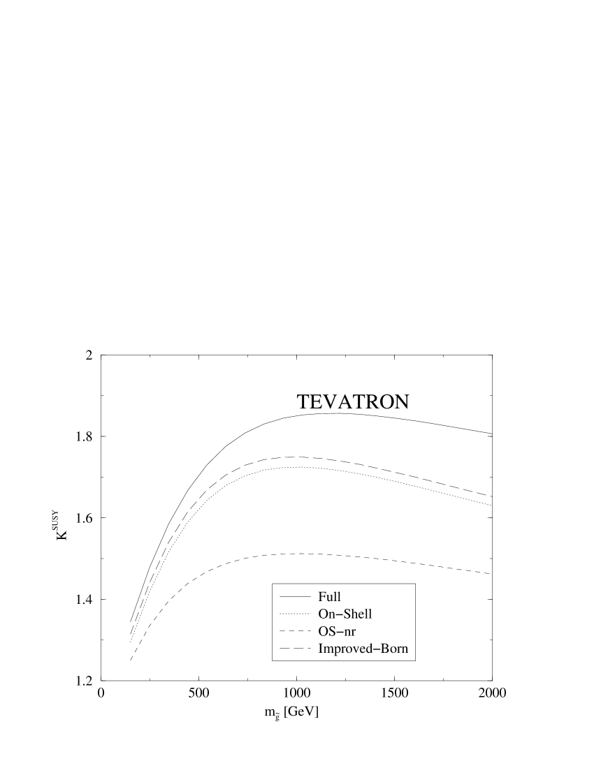
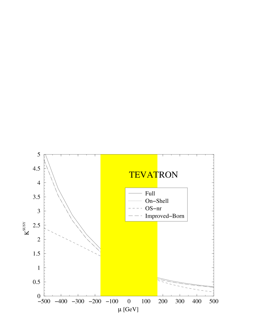
(a)	(b)
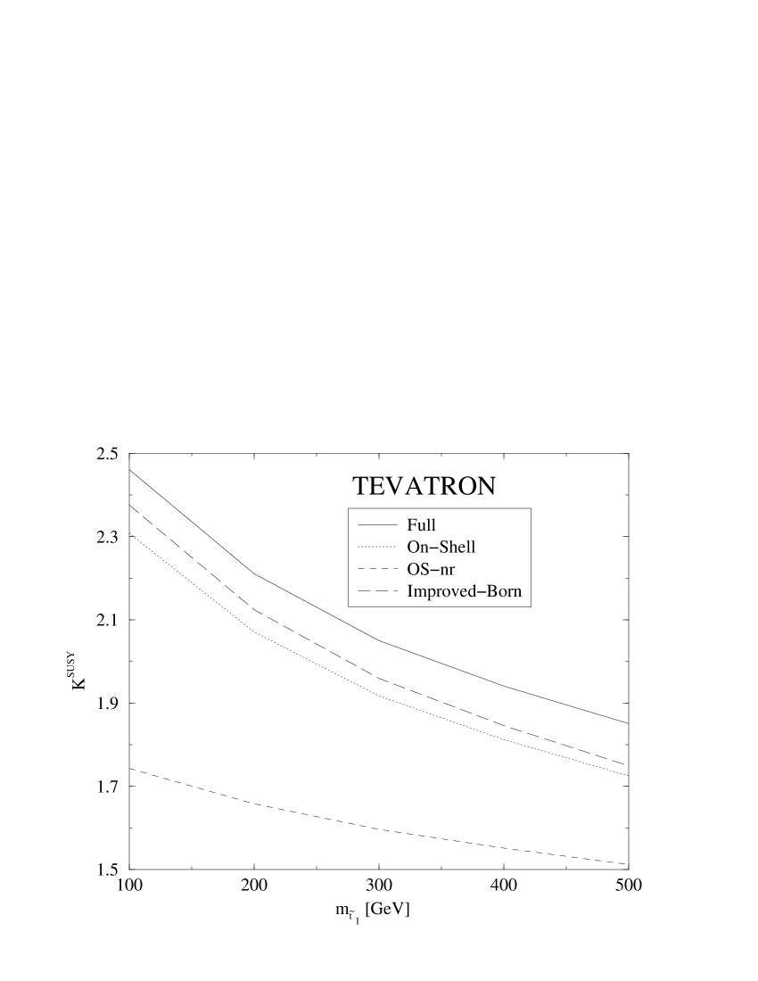
(c)	(d)

Figure 11: $K^{\rm SUSY}$-factor – eq. (36) – for the parameter Set B –Table 6– and $M_{H^{+}}=250\,{\rm GeV}$ at the Tevatron, as a function of a) the gluino mass; b) the $\mu$ parameter; c) the lightest stop mass and d) the top-squark soft-SUSY-breaking trilinear parameter $A_{t}$. Shown are the four approximations explained in the text.

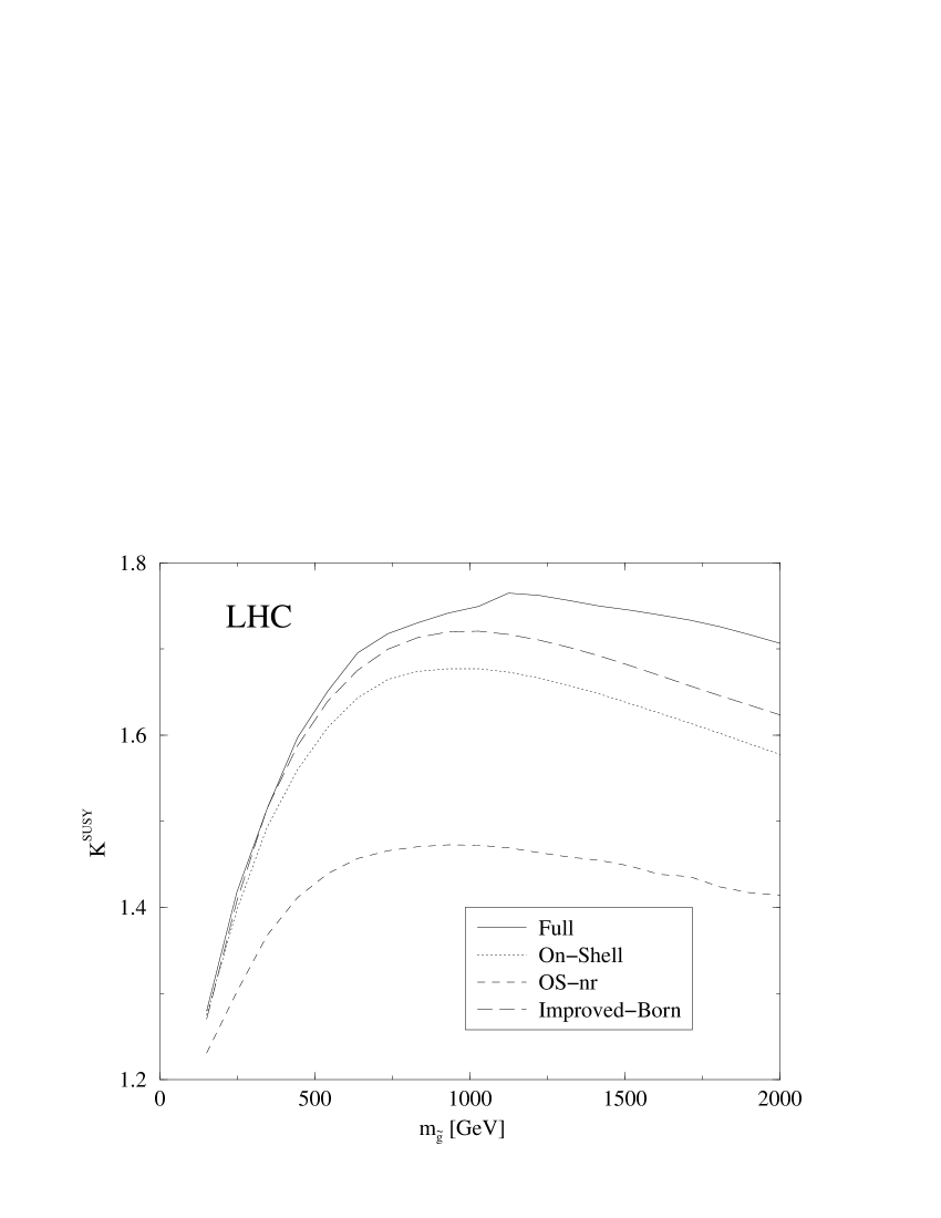
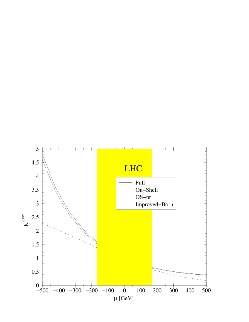
(a)	(b)
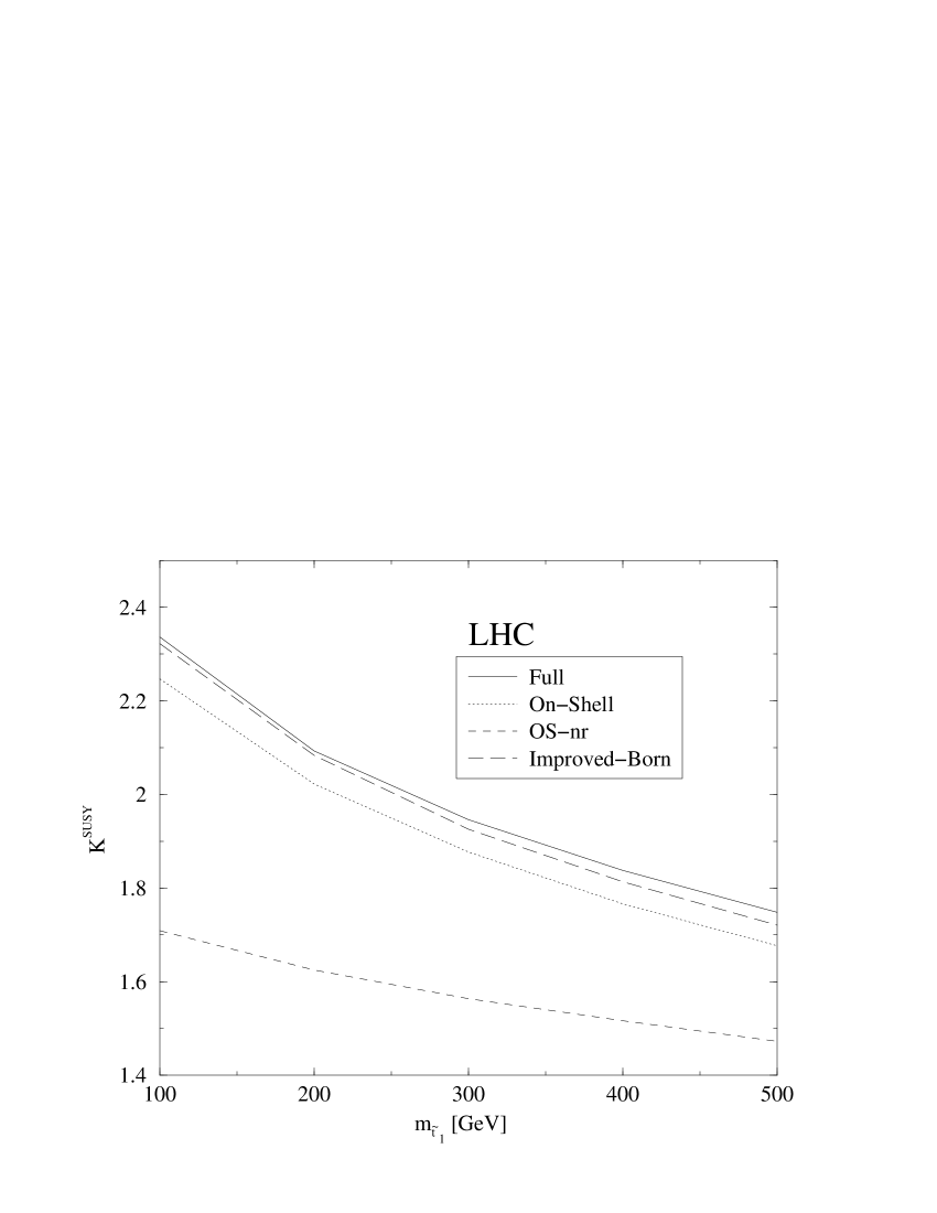
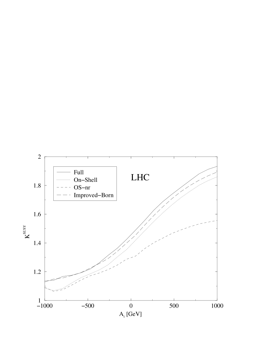
(c)	(d)

Figure 12: $K^{\rm SUSY}$-factor – eq. (36) – for the parameter Set B –Table 6– and $M_{H^{+}}=500\,{\rm GeV}$ at the LHC, as a function of a) the gluino mass; b) the $\mu$ parameter; c) the lightest stop mass; and d) the top-squark soft-SUSY-breaking trilinear parameter $A_{t}$. Shown are the four approximations explained in the text.

for the different contributions mentioned above. In Fig. 11 we present the evolution of the $K^{\rm SUSY}$-factor (36) as a function of various MSSM parameters for the case of the Tevatron and for a charged Higgs boson mass of $250\,{\rm GeV}$. In Fig. 12 we show the same effective $K^{\rm SUSY}$-factor for the LHC and for a charged Higgs boson mass of $500\,{\rm GeV}$. Both cases look pretty similar, the reason being that the leading corrections (eqs. (26-28), Fig. 8) are insensitive to the charged Higgs boson mass and the energy of the process. For the same reason the main features of the corrections follow closely the pattern already observed in the partial decay widths $\Gamma(t\to H^{+}b)$ [10] and $\Gamma(H^{+}\to t\bar{b})$ [12]. In these figures we have concentrated on the moderate Set B, although larger squark masses will not decrease significantly the corrections, unless there exists a large hierarchy between the masses of the squarks, the gluino and the $\mu$ parameter.

For the parameter Set B, the corrections are always positive. They decouple very slowly with the gluino mass, as seen in Figs. 11a and 12a, so a very heavy gluino does not prevent to have large corrections. In Figs. 11 and 12 the role of the resummation is very clear; failing to include it would lead to completely underestimated cross-sections. The shaded regions in Figs. 11b and 12b correspond to a chargino mass below the LEPII mass exclusion limit. The $\mu$ parameter is also a key parameter in the process under study, since the SUSY-QCD corrections grow linearly with it – Cf. Eq. (26). In the $\mu<0$ scenario the SUSY-QCD corrections to the cross-section are positive: roughly, $\delta\sigma/\sigma\sim-2\,(\Delta m_{b})_{SUSY-QCD}>0$. Notice, however, that in Figs. 11b and 12b, $A_{t}>0$, and so the SUSY-EW corrections add constructively to the SUSY-QCD ones $\delta\sigma/\sigma\sim-2\,(\Delta m_{b})_{SUSY-EW}>0$. In the $\mu<0$ and $A_{t}<0$ scenario, instead, the SUSY-EW corrections would partially compensate the positive SUSY-QCD loops, giving a $K^{\mathrm{SUSY}}$ factor slightly smaller. Finally, there is the case $\mu>0$ and $A_{t}>0$, where the two SUSY effects on the cross-section would be negative: $K^{\rm SUSY}<1$. As we have already mentioned, this could lead to $K^{\rm MSSM}\simeq 1$ in eq.(14) and then the signature of the underlying SUSY would be that the QCD corrections are “missing” or even negative! While this is possible for an $Ht\bar{t}$ final state [47], for example due to Coulomb exchange of gluons between quasistatic top quarks, this is not allowed in the presence of $b$-quark in final states at high energies.

We come now to the effects from the squark sector. In Figs. 11c and 12c we show the evolution with the corrections with the lightest stop-quark mass. The plots end at $m_{\tilde{t}_{1}}=500\,{\rm GeV}$ because for larger stop-quark masses there is no physical solution for the mixing angle (given $m_{\tilde{b}_{1}}=500\,{\rm GeV}$) in this particular set of inputs. We see that, although the corrections have a dependence on the squark masses, this parameter is not the most critical one. In fact, we emphasize that larger squark masses (as e.g. $m_{\tilde{b}_{1}}\simeq m_{\tilde{t}_{1}}\simeq 1\,{\rm TeV}$) do not necessarily lead to smaller corrections – see Fig. 9, parameter Set A.

We finally focus on the influence of the soft-SUSY-breaking trilinear stop-quark coupling $A_{t}$ (Cf. Figs. 11d and 12d), which is another key parameter for the corrections under study. We see that, again, the preferred range ($\mu<0,A_{t}>0$) gives the largest positive corrections, thus enhancing the total cross-section dramatically.

(a)	(b)

Figure 13: $K^{\rm SUSY}$-factor – eq. (36) – for the parameter Set B –Table 6– for the different production channels as a function of $\tan\!\beta$: a) For the Tevatron, and $M_{H^{+}}=250\,{\rm GeV}$ and b) the LHC and $M_{H^{+}}=500\,{\rm GeV}$.

The final point that we wish to address is the study of the relative contributions from the different channels involved in the production cross-section –eqs. (2)-(4). Since the main effect comes from the $\Delta m_{b}$ term, we expect that the SUSY-corrections will be very similar in all the channels. In Fig. 13 we display the corrections from the different channels for the Tevatron and the LHC. We see, indeed, that the corrections to the various channels are very similar. This means that to obtain the discovery potential (or exclusion region) for the different accelerators in the presence of the SUSY-corrections, we may directly scale up the previous results from Fig. 7 by a factor $K^{\rm SUSY}$ without having to remake the full kinematical analysis.

4.3 Consequences for the charged Higgs boson search

In the previous figures 9-12 we have exemplified a wide variety of MSSM effects on the cross-section of process (1) based on a typical set of MSSM inputs (sparticle masses and soft-SUSY-breaking parameters). The new contributions entail cross-section enhancements at the level of $50-70\%$ beyond standard QCD expectations. In other words, the SUSY loops have the capability to modify the largest expected QCD $K$-factor from $K_{\max}^{\rm QCD}=1.6$ up to an effective MSSM value (14) reaching $K^{\rm MSSM}=2.4-2.7$. Surely enough, if such a dramatic effect is really there, it could not be experimentally missed. In turn the discovery and exclusion limits on the charged Higgs boson inferred from the previous analysis will get significantly modified as compared to the tree-level case (Cf. Fig. 7), as we shall see next.

As already warned in Section 3.1, one should also keep in mind the SUSY corrections to the branching ratio $BR(H^{+}\to t\bar{b})$. They are certainly much tamed than those potentially affecting the partial decay width $\Gamma(H^{+}\to t\bar{b})$ [77], but even so they can have some impact on the charged Higgs boson mass discovery/exclusion limits. Recall that the QCD corrections decrease significantly the partial decay width $\Gamma(H^{+}\to t\bar{b})$ [77]. The genuine SUSY corrections, on the other hand, are governed by the same kind of contributions discussed in this paper, and can therefore have both signs [12, 35]. As the sign of the SUSY quantum effects on the branching ratio is the same as for the production cross-section, they just mutually enhance or suppress the signal. Here we use the improved expression for this partial decay width given in Ref. [35]. The only other decay channel that we consider is $H^{+}\to\tau^{+}\nu_{\tau}$, but we neglect the SUSY corrections to its partial decay width. Notice that, since $BR(H^{+}\to t\bar{b})$ is much larger than $BR(H^{+}\to\tau^{+}\nu_{\tau})$, the quantum corrections to the branching ratio $BR(H^{+}\to t\bar{b})$ will be small in general. We remark that in the light charged Higgs boson mass scenario relevant to our $t\bar{t}b\bar{b}$ signature (viz. $m_{t}+m_{b}<M_{H^{\pm}}<300\,{\rm GeV}$), the partial decay channel $H^{+}\to\tau^{+}\nu_{\tau}$ has a sizeable branching ratio which raises very fast with decreasing $M_{H^{\pm}}$. For instance, for $M_{H^{\pm}}\sim(230-240)\,{\rm GeV}$ and a moderately high $\tan\!\beta=30$ one gets $BR(H^{+}\to\tau^{+}\nu_{\tau})\gtrsim 20\%$ (without SUSY corrections). In some cases (specifically when $\mu>0,A_{t}<0$, like in Sets C and D in Table 6) this branching ratio can be further enhanced by SUSY effects due to the corresponding decrease of $\Gamma(H^{+}\to t+\bar{b})$. Thus for charged Higgs masses in the heavy range ($M_{H^{\pm}}>300\,{\rm GeV}$), where the uncorrected branching ratio of the $\tau$-mode would be below $10\%$, the latter can actually remain at the level of $15\%$ (even for $M_{H^{\pm}}\gtrsim 500\,{\rm GeV}$) thanks to the SUSY effects; this scenario would be realized e.g. for $(m_{\tilde{g}},m_{\tilde{t}_{1}},m_{\tilde{b}_{1}},\mu,A_{t},A_{b})\simeq(500,150,300,200,-200,200)\,{\rm GeV}$ at $\tan\!\beta=30$ as before. Hence, it is clear that there are situations for $M_{H^{\pm}}\gtrsim m_{t}-m_{b}$ where the $\tau$-mode could be successfully used to explore the light charged Higgs mass region, as it was already the case in Run I for $M_{H^{\pm}}<m_{t}-m_{b}$ through the study of the combined decay $t\rightarrow H^{+}+b\rightarrow\tau^{+}\nu_{\tau}+b$ [14, 15, 16, 17]. Nevertheless, the $\tau$-mode can alternatively be highly suppressed by the SUSY effects themselves – if they turn out to greatly enhance $\Gamma(H^{+}\to t+\bar{b})$. Indeed, for $(m_{\tilde{g}},m_{\tilde{t}_{1}},m_{\tilde{b}_{1}})\simeq(500,150,500)\,{\rm GeV}$ and assuming $(\mu,A_{t},A_{b})$ as in Sets A and B, the $\tau$-decay of the charged Higgs narrows down to a $5\%$ or less. Therefore, the SUSY suppression of the $\tau$-mode turns out to occur in the regions of the MSSM parameter space where the production processes $p\bar{p}(pp)\to H^{+}\bar{t}b+X$ are maximized. We conclude that in the parameter space relevant for $p\bar{p}(pp)\to H^{+}\bar{t}b+X$ the $t\bar{t}b\bar{b}$ signature is in general the most suited one, and indeed it is the only one used in the present study. We warn the reader that at the opposite end of the spectrum, where $M_{H^{+}}\stackrel{{\scriptstyle\scriptstyle>}}{{{}_{\sim}}}1\,{\rm TeV}$, the branching ratio $BR(H^{+}\to t\bar{b})$ would significantly decrease if $M_{H^{+}}>m_{\tilde{b}_{1}}+m_{\tilde{t}_{1}}$, due to the opening of the squark decay channels $H^{+}\to\tilde{b}_{i}\tilde{t}_{j}$ – which quickly become dominant at high $\tan\!\beta$. Given the parameters in Table 6, these squark channels are relevant only for $M_{H^{+}}>1\,{\rm TeV}$ (resp. $2\,{\rm TeV}$) for the parameter Sets B and C (resp. A and D). Since these squark channels have not been considered in the present study, the conclusions on the charged Higgs boson discovery/exclusion limits are strictly valid only for $M_{H^{+}}<m_{\tilde{b}_{1}}+m_{\tilde{t}_{1}}$. While we could easily include the new $H^{+}$ decay modes, the typical results from our study would not change at all. In fact, we have emphasized that the leading SUSY corrections relevant for our process do not necessarily decrease with the SUSY mass scale, so that our numerical results can be extended to $M_{H^{+}}>1\,{\rm TeV}$ since we can always find a modified particle spectrum satisfying $M_{H^{+}}<m_{\tilde{b}_{1}}+m_{\tilde{t}_{1}}$ and producing the same radiative corrections as the corresponding parameter set in Table 6.

In Fig. 14 we show the equivalent of Fig. 7, but using the full SUSY-corrected cross-section, and the corrected branching ratios, for $\tan\!\beta=50$. In the Tevatron case, whose tree-level cross-section borders the discovery limits from below, we have applied a QCD correction factor $K^{\rm QCD}=1.5$ to account for the (yet unknown) standard QCD corrections to the production cross-section. Without large QCD corrections, the Tevatron cannot discover a heavy charged Higgs boson $M_{H^{+}}>200\,{\rm GeV}$ (not even at a $3\sigma$ level of significance) unless the SUSY corrections are as high as e.g. those corresponding to Set A in Table 6. In this case a charged Higgs boson in the range $M_{H^{+}}\lesssim 255\,{\rm GeV}$ can still be discovered at $3\sigma$ at the Tevatron. This is certainly a welcome possibility as it would throw light on the SUSY nature of that charged Higgs boson, in case of being detected, and in addition it would strongly hint at regions of the MSSM parameter space very much akin to those defined by Set A. On the other hand, for intermediate SUSY sets (like Set B), the concurrence of the QCD corrections is indispensable to get a similar charged Higgs boson signal. At the LHC, in contrast, large discovery/exclusion regions exist already using the tree-level approximation ($K^{\rm QCD}=1$), so we are more conservative in this case and we can afford not to apply a $K^{\rm QCD}$ correction factor. The band in Fig. 14 interpolates the parameter space between the parameter sets A and D –Table 6–, which can be regarded as plausible parameter sets defining the typical range of maximum and minimum cross-sections expected in the MSSM. The interpretation of this figure is as follows: in the context of the MSSM, and within the representative region of parameter space discussed in Section 4.1, the Tevatron should be able to discover a relatively heavy charged Higgs boson ($M_{H^{+}}\stackrel{{\scriptstyle\scriptstyle<}}{{{}_{\sim}}}250\,{\rm GeV}$) at the canonical $5\sigma$ significance only in an scenario of very large positive SUSY corrections. Nonetheless, the Tevatron can still find some reasonable evidence (at $3\sigma$, i.e. $99.7\%$ C.L.) of a charged Higgs boson with a mass $200-250\,{\rm GeV}$ if only the condition $\mu<0$ applies irrespective of the sign of $A_{t}$. The LHC, on the other hand, does guarantee a $5\sigma$ discovery in the range $M_{H^{+}}<800\,{\rm GeV}$ for $100~{}{\rm fb}^{-1}$ of integrated luminosity; and a $3\sigma$ evidence of a charged Higgs boson with a mass up to $1\,{\rm TeV}$ for any SUSY spectrum. With only $30~{}{\rm fb}^{-1}$ the LHC can not discover a superheavy charged Higgs boson $M_{H^{+}}>1.1\,{\rm TeV}$, but the discovery is possible for $M_{H^{+}}<1.1\,{\rm TeV}$ and $\mu<0$. Once we will have data from the LHC this picture could change significantly. If SUSY particles are found, and we know (roughly) their mass scale, the band in Fig. 14 will get significantly shrunk, providing clean predictions. If, on the contrary, a charged Higgs boson is found, but the scale of the SUSY particles is still not known with sufficient accuracy, one can use Fig. 14 to extract information on the SUSY particles properties. Clearly the potential impact of the SUSY corrections is not at all negligible and should not be ignored in any serious analysis of this subject.

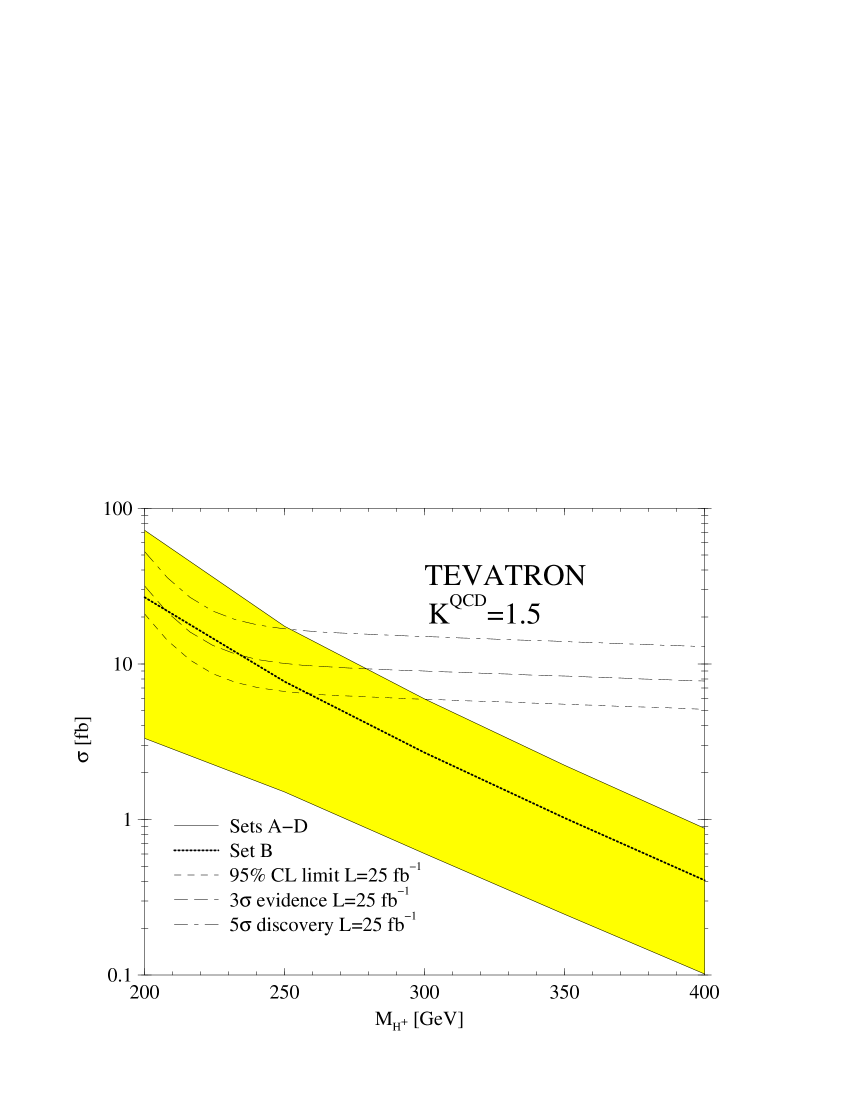
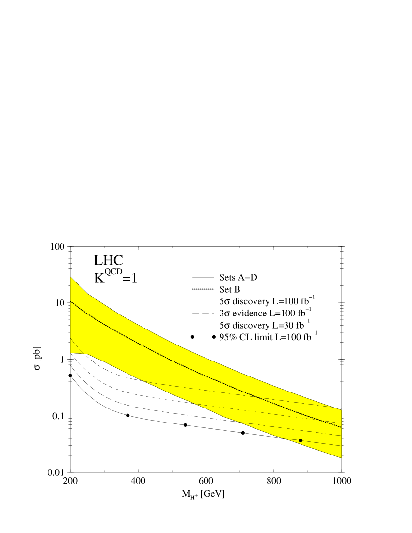
(a)	(b)

Figure 14: Total effective cross-section for the process (1) as a function of the charged Higgs boson mass a) at the Tevatron with a QCD correction factor $K^{\rm QCD}=1.5$ and b) the LHC (with $K^{\rm QCD}=1$). In both cases $\tan\beta=50$. Shown is the total cross-section interpolating between parameters sets A and D (shaded region) and for the parameter Set B. Also shown are the cross-sections necessary for discovery and exclusion from Fig. 7.

By iterating this procedure we find the regions of the $\tan\!\beta-M_{H^{+}}$ plane in which each experiment can find (or exclude) the existence of the charged Higgs boson. We present the result of this analysis in Figs. 15a and b. These figures make transparent what was stated above: the presence of the SUSY corrections alters significantly the Higgs boson discovery potential of the hadron colliders. From the figures it is also patent the Tevatron could have a non-negligible chance to find a charged Higgs boson in the intermediate range $M_{H^{\pm}}<280\,{\rm GeV}$.

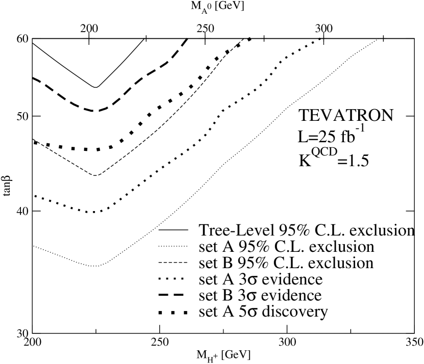
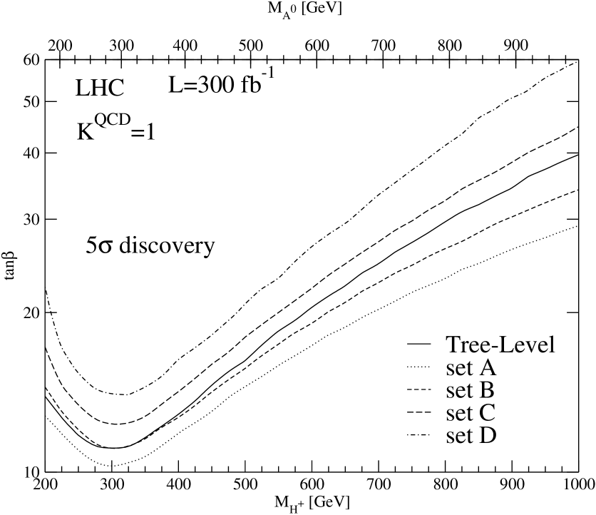
(a)	(b)

Figure 15: Discovery/Exclusion regions for the Tevatron and the LHC, in the $\tan\!\beta-M_{H^{+}}$ plane. Also shown is the value of $M_{A^{0}}$ corresponding to each $M_{H^{+}}$ according to the MSSM.

We have also shown in Fig. 15 the value of the pseudoscalar Higgs boson mass $M_{A^{0}}$ corresponding to each value of $M_{H^{+}}$. We have correlated $M_{A^{0}}$ with $M_{H^{+}}$ using the one-loop corrections to the Higgs bosons masses as provided by the program FeynHiggsFast [78]. Note that in this case $M_{H^{+}}$ changes with $\tan\!\beta$, but is also different for each set of SUSY parameters. However, the change of $M_{A^{0}}$ among the different sets is very small (below 5%), and the one-to-one correspondence $M_{H^{+}}\leftrightarrow M_{A^{0}}$ is a very good approximation.

Since the performed analysis of the SUSY corrections is meaningful only for large $\tan\!\beta$  ($\tan\!\beta\stackrel{{\scriptstyle\scriptstyle>}}{{{}_{\sim}}}20$), the shifts in the discovery regions in Fig. 15b are not sufficiently reliable for $\tan\!\beta\stackrel{{\scriptstyle\scriptstyle<}}{{{}_{\sim}}}20$. Unfortunately this means we can not compare with the results of Ref. [3], given for $M_{A^{0}}<500\,{\rm GeV}$ (which correspond to $\tan\!\beta$  values $\lesssim 20$ in Fig. 15b). Sticking to the large $\tan\!\beta$  scenario, we see that for $\tan\!\beta=60$ a charged Higgs boson discovery is guaranteed for $M_{H^{+}}<1\,{\rm TeV}$. For $\mu<0$ a charged Higgs boson could be discovered up to a mass of $1\,{\rm TeV}$ for any $\tan\!\beta>30$.

We should also recall here that our results show a certain degree of uncertainty due to the dependence of the cross-sections on the particular PDF parametrization and the variation with the renormalization and factorization scales, which we have already illustrated in section 3. These issues are particularly relevant for the Tevatron, where a charged Higgs boson of order $250\,{\rm GeV}$ could be discovered only if the QCD and SUSY effects add up with the same positive sign. In the worst possible scenario, the $K^{\rm QCD}=1.5$ factor that is needed in combination with the typical SUSY effects from the parameter Set B in Table 6 could be effectively reduced. In this adverse circumstance the charged Higgs discovery at the Tevatron would only be possible if the SUSY effects would be still larger, namely at least as large as those from the parameter Set A in that table. In any case the lesson is once again the same: without the collaboration of SUSY (or some other form of physics beyond the SM), the charged Higgs discovery is impossible at the Tevatron. On the other hand, the aforementioned uncertainties are much more tamed for the LHC, and our results shown in Fig. 14b and 15b should not be too much affected by them.

5 Summary and conclusions

We have presented a thorough study of the process $p\bar{p}(pp)\to H^{+}\bar{t}b+X$ in hadron colliders in order to assess the possibility to see a SUSY charged Higgs boson at the Tevatron II and at the LHC. A necessary starting condition for this is that $\tan\beta$ is sufficiently large (viz. $\tan\beta>20$) so as to insure that the cross-section of the process $p\bar{p}(pp)\to H^{+}\bar{t}b+X$ is sizeable. Beyond this tree-level requirement, our study of the quantum corrections to that process within the MSSM has shown that they are dominated by exceptionally important effects that can be absorbed into an effective $tbH^{+}$ vertex, and therefore in practice they can be treated at the level of an “improved Born approximation”. After the inclusion of the MSSM effects we have found that the “effective $K$-factor” (14) for the process $p\bar{p}(pp)\to H^{+}\bar{t}b+X$ could be either smaller than expected, perhaps barely $K^{\rm MSSM}\lesssim 1$, or on the contrary substantially higher, say $K^{\rm MSSM}=2-3$. In both cases it should be possible to exploit this process to unravel the nature of the new physics in which the purportedly discovered charged Higgs boson is integrated. This could be performed by detecting the existence of large radiative corrections beyond the SM, namely sizeable quantum effects that remain after subtracting the full set of conventional QCD corrections at the NLO. This will typically be the case if the squark masses are heavy at an intermediate level of order of a few hundred $\,{\rm GeV}$. The gluino, notwithstanding, can be as heavy as $1\,{\rm TeV}$. Remarkably enough, in certain circumstances explained in the text all the sparticle masses, and not only the gluino, could be of order of $1\,{\rm TeV}$, and still the MSSM quantum effects would remain large ($\sim 50\%$). This feature shows that sound hints of SUSY can be derived from the sole study of Higgs boson production even if the whole sparticle spectrum is barely accessible to the future colliders.

If $\tan\beta\gtrsim m_{t}/m_{b}>35$, then the upgraded $2\,{\rm TeV}$-Tevatron can exclude charged Higgs boson masses below $300\,{\rm GeV}$ at the $95\%$ C.L. On the other hand, it is not likely that the Tevatron will be able to produce any signal at the $5\,\sigma$ significance level to “officially” discover a SUSY charged Higgs boson. The only chance would be in the narrow window $M_{H^{+}}=(180-250)\,{\rm GeV}$ and assuming the most favorable region in the MSSM parameter space (typically, Set A in Table 6). In any case, the Tevatron can provide reasonable evidence (at the $3\,\sigma$ level) of a $M_{H^{+}}=(200-300)\,{\rm GeV}$ Higgs boson, and also it can do a good complementary job at high $\tan\beta$ using the neutral Higgs bosons channels $p\overline{p}(pp)\rightarrow h\,\overline{b}b+X$ ($h=h^{0},H^{0},A^{0}$) already studied in the literature  [2, 3, 4], where the absence of a top quark in the final state increases the signal in some of them provided the Higgs boson is not too heavy. In this respect we have seen that in the light charged Higgs boson mass scenario, the partial decay channel $H^{+}\to\tau^{+}\nu_{\tau}$ has a large branching ratio, and in some favorable cases it could be successfully used at the Tevatron II to explore this region, as it was the case for the Run I [14, 15, 16, 17]. Fortunately, the situation with the LHC is much more rewarding under similar circumstances. In fact, the LHC will be able to discover a charged Higgs boson up to $800\,{\rm GeV}$ or else to exclude it up to $1\,{\rm TeV}$ at least. Remarkably, these limits can be significantly improved up to $1.1\,{\rm TeV}$ and $1.5\,{\rm TeV}$ respectively in the presence of SUSY corrections.

At the end of the day the strategy should be clear and can be put in a nutshell. If the signal $p\bar{p}(pp)\to H^{+}\bar{t}b+X$ is found it will automatically imply new physics. Moreover, under the assumption that the discovered charged Higgs boson is a member of a Type II two-Higgs-doublet model it will strongly suggest a high value of $\tan\beta$, certainly not below $20$, and most likely above $30$. Then an accurate measurement of the $tbH^{+}$ vertex should be possible at a level better than $10\%$, together with its correlation with the neutral Higgs bosons vertices $\overline{b}bh$ ($h=h^{0},H^{0},A^{0}$) obtained both at the LHC and at the Tevatron from the measurement of the companion processes $p\overline{p}(pp)\rightarrow h\,\overline{b}b+X$. After subtraction of the conventional QCD corrections the genuine non-standard quantum effects could possibly be disentangled after accurate comparison of all these signals [31, 36]. As we have shown, the “remnant” of this subtraction could be quite large in the MSSM case, viz. of the order of the full QCD effects themselves! Then a pattern of sparticle masses (or at least of favoured regions in the MSSM parameter space) responsible for these virtual effects could emerge (see e.g. figures 9-12), and of course it should be cross-checked with the results obtained from other independent experiments, e.g. at the LC [32]. Altogether the bottom line of this strategy could definitely point towards the supersymmetric nature of the found Higgs bosons until the sparticles themselves will eventually be produced and correctly identified.